1. Introduction
Organic Rankine Cycles (ORCs) have been increasingly applied to produce electricity from low and medium temperature sources in the last decade. The reported global installed capacity has currently surpassed 2700 MW
e, and an additional 523.6 MW
e have been planned [
1]. Typical application fields for ORC are geothermal, biomass, solar thermal and low grade waste heat recovery plants [
2,
3,
4]. The size of ORC plants can vary from few kW
e to some MW
e [
4,
5]. Several studies report the advantages of organic fluids in comparison to water for low and medium temperature small-size power plants [
5,
6,
7]. As an example, in [
8,
9] the organic fluid resulted to be better performing than water and air for a heat source temperature below 300 °C.
Given the modest temperature of the source, the electrical efficiency of ORCs is generally less than 20% [
2,
4]. The remaining energy is either dissipated through piping, compression and expansion machines, heat losses, auxiliary consumption and heat transfer to the condenser. The heat rejected to the condenser can be recovered to provide thermal energy for district heating, commercial buildings and industrial processes. In this case, the ORC is designed to work in combined heat and power (CHP) mode, providing electricity and heat with a relatively high energy utilization factor [
10,
11,
12]. A comparison of the different configurations for ORC in CHP mode is provided in [
13].
A simple ORC system consists of four main elements: a preheater/evaporator, where the working fluid is preheated and vaporized at saturated state or slightly superheated, an expansion machine, where the thermal energy of the fluid is converted into rotational energy of the expander shaft, a condenser, where the fluid is cooled down and condensed back to liquid state, and a pump, which brings the condensed liquid to the evaporation pressure to start the process cycle again. A recuperator might be applied, being advantageous mainly for dry fluids. Sub-, trans- and supercritical ORCs with pure organic fluids and their mixtures have also been investigated [
14,
15,
16,
17,
18,
19,
20,
21]. Supercritical ORCs might offer higher system efficiencies in dependency of the temperature source, at the expenses of higher investment and maintenance costs. The reduced temperature difference at the evaporator causes higher investment costs, because of the larger heat transfer surface and the higher pressure that the evaporator has to withstand [
15,
22]. For dry fluids, superheating has no positive effect and should be avoided, since it increases the complexity of the evaporator and the thermal stresses on the expansion machine [
23].
The evaporator is the crucial component that links the ORC to the heat source/heat transfer medium, and its design is therefore of major relevance for the thermodynamic, hydraulic and economic performance of the ORC. For mobile applications, the heat exchanger has to be additionally optimized in terms of volume and weight [
24,
25,
26].
In the following, the main configurations of evaporators for stationary ORC are considered. Fin-and-tube heat exchangers are mainly applied for waste heat recovery from gas turbine and internal combustion engines [
27,
28,
29]. The extended surface of the shell side improves the heat transfer for the exhaust gas, whereas the working fluid shows a heat transfer coefficient of at least two orders of magnitude higher and flows inside the tubes [
28]. The pressure drop of the exhaust gas on the shell side has a negative impact on the performance of the topping cycle and should be minimized [
30,
31,
32]. Shell-and-tube heat exchangers are applied or assumed for ORC optimization in different studies [
33,
34,
35,
36]. This type of heat exchanger can be deployed up to very high pressures and temperatures, has a relatively simple geometry and its design and manufacturing procedures are very well-known and established [
37]. Plate heat exchangers might be advantageous for low pressure, low temperature applications thanks to their compactness, effectiveness, easiness to be cleaned, maintained or extended [
38]. As a major drawback, plate heat exchangers increase the pressure losses, especially for exhaust gas waste heat recovery, because of the narrow channels. A comparison between shell-and-tube and plate heat exchangers is carried out in [
39].
In large size subcritical ORCs, kettle boilers are often used as evaporators [
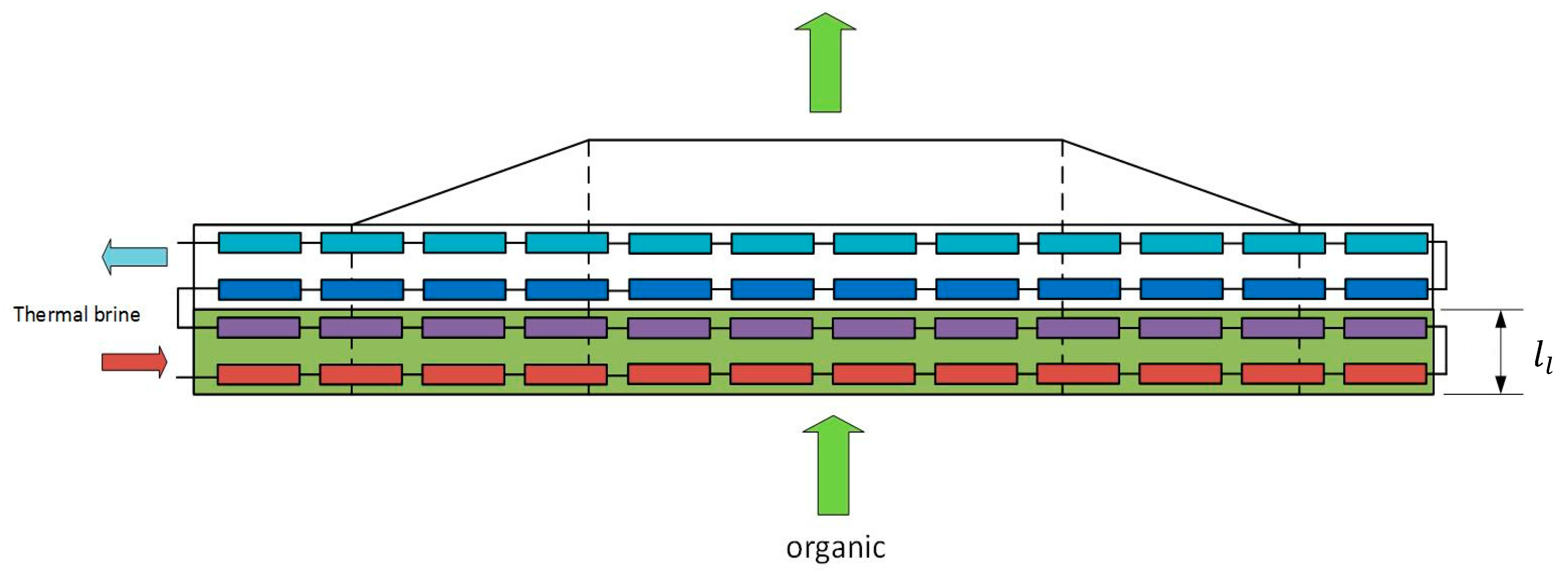
6]. The preheating of the organic fluid generally occurs in once-through shell-and-tube heat exchangers, whereas the evaporation takes place in the kettle boiler. The heating fluid, e.g., thermal brine for a geothermal power plant, passes through the tubes in a single- or multi-pass scheme. If no superheating is desired, the tube bundle is completely submerged in the liquid pool. The boiler disposes of a freeboard at the top of the kettle for separation of the vapor and liquid phase [
37]. The vapor is then extracted from the top of the boiler, and fed to the expander. The effective separation between liquid and vapor in a kettle boiler gives more flexibility in power plant operation. In fact, in case of sudden variation of the input source, the boiler responds with a variation in pressure and/or level, avoiding that droplets get entrained to the turbine inlet [
40]. In off-design conditions, some tubes may lay above the liquid level, leading to some degree of superheating and hence ensuring that no droplets are carried out to the expander inlet. In case of tube exposed to the vapor, tube material limits should not be overcome as a result of the higher wall temperature. The dynamic flexibility gives a significant advantage to kettle boilers with respect to tube once-through boilers. In the latter some degree of superheating is always necessary for safety reason, and a more demanding control is required to ensure pure vapor conditions at the expander inlet [
40]. The pool boiler configuration is also recently being mentioned for mixtures of organic fluids [
40]. An accurate evaporator design has also to consider the response of the heat exchanger in transient conditions. Dynamic simulations of ORC power plants are, in fact, gaining significant interest for a number of reasons:
To increase the energy conversion efficiency, power plants must be able to respond very fast and in an optimal way to variations in heat source or ambient conditions (e.g., waste heat recovery systems);
Control strategies can be improved, e.g., shifting from classical PID controllers [
41,
42] to advanced model-based or model-predictive strategies, leading to higher energy recovery [
43,
44,
45];
The presence of hot spots in heat exchangers during transients can be limited, avoiding thermal degradation of the working fluid [
46];
The increasing complexity in the dynamics of the electricity grid, associated with the increasing penetration of variable-source renewables (i.e., wind and photovoltaics), requires a higher contribution from controllable power plants (biomass, geothermal) for security margin, load reserve and grid stability;
Renewables-based ORCs could be used as stand-alone systems in remote areas and operated under strong dynamic conditions [
47];
The design of systems operated most of the time in off-design conditions (e.g., waste heat recovery) could be improved; stresses and plant lifetime can be increased [
48,
49];
Start-ups, shutdowns and emergency situations (turbine trips, safety valve lifting) can also take help from dynamic simulations [
50].
Dynamic models of ORC have been mainly developed in the Modelica
® language (Modelica Association, Linköping, Sweden) [
51]. The equation-based, object-oriented and a-causal nature of the modelling language makes it very suitable for simulation of nonlinear thermo-fluid systems, such as ORC power plants [
47,
52]. The different plant components are developed as “individual objects” which can be connected to each other. The objects are generally compiled in libraries. Different libraries for thermo-fluid systems are available, either open-source or commercial [
53]. Several software codes based on this modelling language are available, such as Dymola, SimulationX, JModelica or OpenModelica [
54]. Thermodynamic and transport properties of the fluid are generally accessed by means of external fluid property libraries, e.g., NIST Reference Fluid and Transport Properties Database (REFPROP), FluidProp, CoolProp or TILMedia [
55,
56,
57,
58]. The focus of these dynamic tools is generally on the overall plant performance and the interaction among components rather than on the detailed description of the single elements, which is generally carried out with more demanding tools, such as Computational Fluid Dynamics (CFD) or Finite Element Methods (FEM) [
47].
The broad application of kettle boilers for middle and large size ORCs, together with the increasing interest in ORC dynamics and simulation, require a valid model for the dynamic simulation of this component. The complex geometrical arrangement makes also current models unsuitable for this scope. In this paper, a dynamic model of a kettle evaporator is developed and validated with measured data. The model has the advantage of high simulation speed, good accuracy and a high flexibility for different heat exchanger geometries.
The dynamic modelling of heat exchangers and in particular evaporators for ORC systems is discussed in the next section. A closer insight into the proposed model for the kettle boiler is gained in
Section 2. Validation and results are reported in
Section 3, followed by a discussion in
Section 4. A brief summary and conclusions are found at the end of this paper.
Dynamic Modelling of Evaporators for Organic Rankine Cycles
Dynamic models of heat exchangers (and not only) are based on the principle laws of mass, energy and momentum conservation, and integrated by empirical correlation to account for specific properties or characteristics of the system. The models are typically discretized over the length of the heat exchangers (1-D). The choice of the state variables for fluid property computation is discussed in [
59,
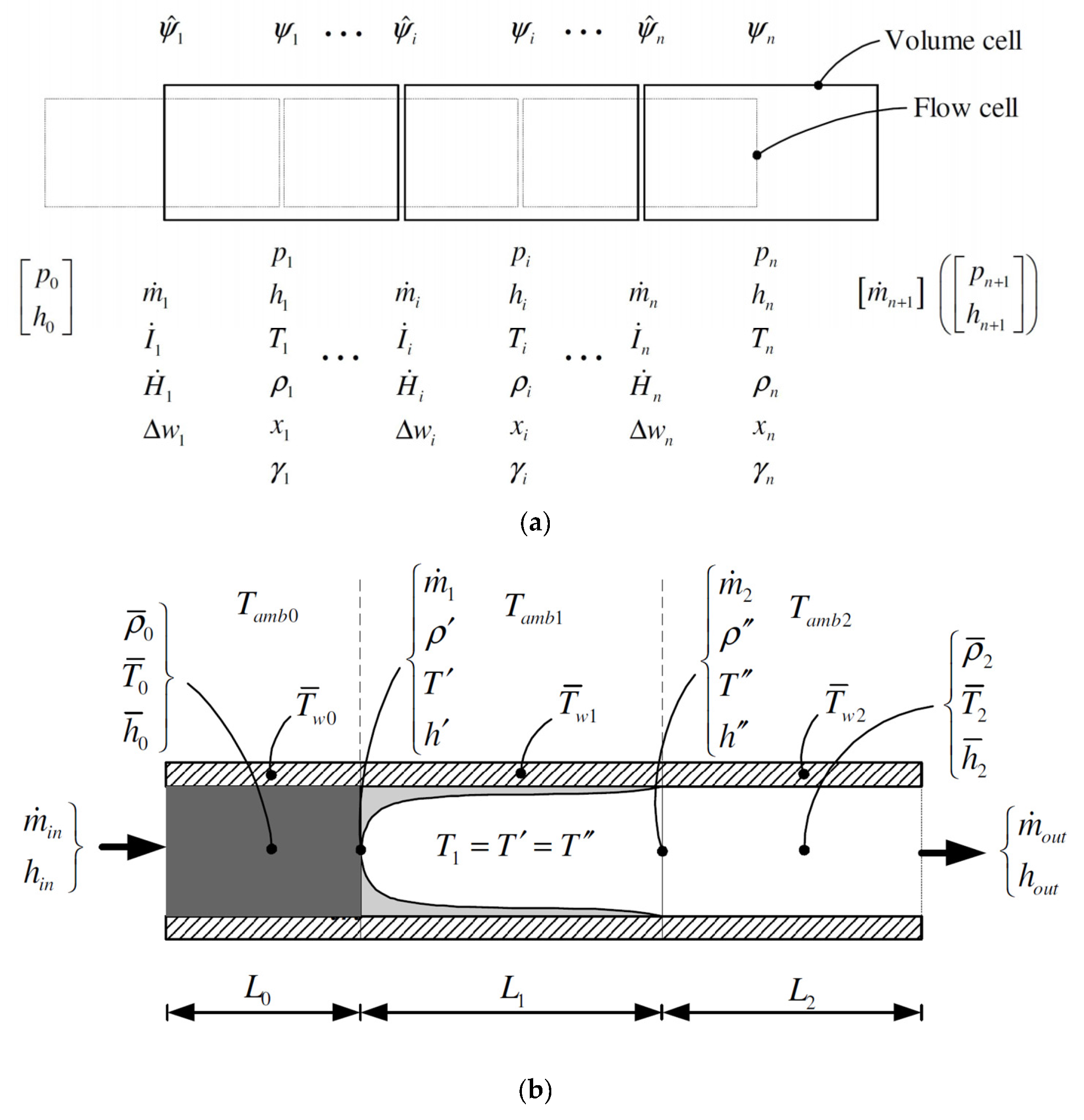
60]. The state variables have a strong impact on how the differential-algebraic equations (DAE) are solved. Most of the tools nowadays use pressure and specific enthalpy as state variables. The state of the solid wall of heat exchangers is defined by the wall temperature. The way the equations are numerically solved defines the type of dynamic model used for the heat exchanger. The most common types are (conceptually depicted in
Figure 1):
Finite volumes (FV);
Moving boundary (MB).
The FV method is based on a static discretization of the heat exchanger in a given number of cells of equal volume. According to the degree of subcooling at the inlet and/or superheating at the outlet of the heat exchanger, the fluid in a cell can be in liquid, vapor or two-phase. On one hand, a higher number of cells is generally desired for higher accuracy of the solution. On the other hand, the computational time increases with the number of cells. A trade-off has to be found between the accuracy of the solution and the computational time. A major problem occurs with the FV method applied to a phase-change heat exchanger. This can be explained looking at the continuity equation:
where
is the fluid density,
the cell volume,
the incoming and
the outgoing fluid mass flow rate. Since the saturated liquid line shows a large discontinuity in density when the fluid passes from the liquid to the two-phase region, the time derivative of the density
can become very high. If the inlet mass flow rate
is given, a fast density change can cause peaks in
resulting in flow reversal, chattering or non-solvable solutions. The simulation can become extremely slow or even fail [
61].
MB refers to fast low-order dynamic models that subdivide the heat exchanger in a liquid, vapor and two-phase control volume. If one of the regions is not present, the corresponding volume is neglected. The volumes dynamically change their length according to the thermodynamic conditions in the heat exchangers. Techniques to account dynamically for the presence of each control volume are also available [
62]. In the two-phase region, the average density
is computed in MB methods by means of the average void fraction, according to [
63]:
where
is the average void fraction, and
and
are the densities of saturated liquid and vapor. Assumptions on the average void fraction have to be made. The validity of the assumption has an impact on the accuracy of the dynamic simulation [
63].
The MB and FV models have been compared in [
59,
63,
64]. The MB model requires less computation time than FV, even though the accuracy is typically lower. The MB model could preferably be applied for online control systems, rather than system simulation [
59,
60]. The computation of the amount of working fluid present in the cycle (also called charge) is critical for both models because of the absence of high-accuracy correlations for the void fraction in the evaporator and condenser. The MB model has however shown worse results between the two [
64].
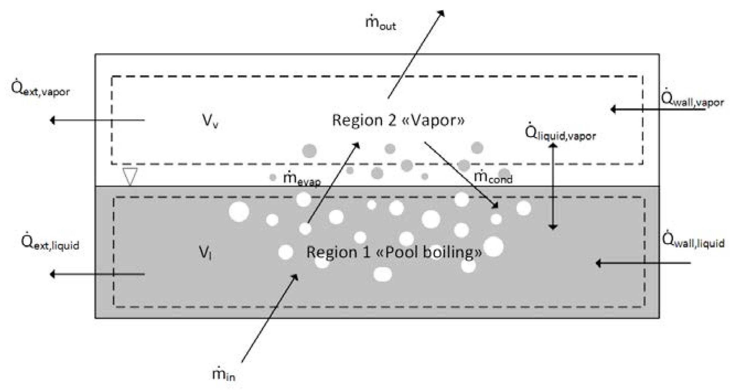
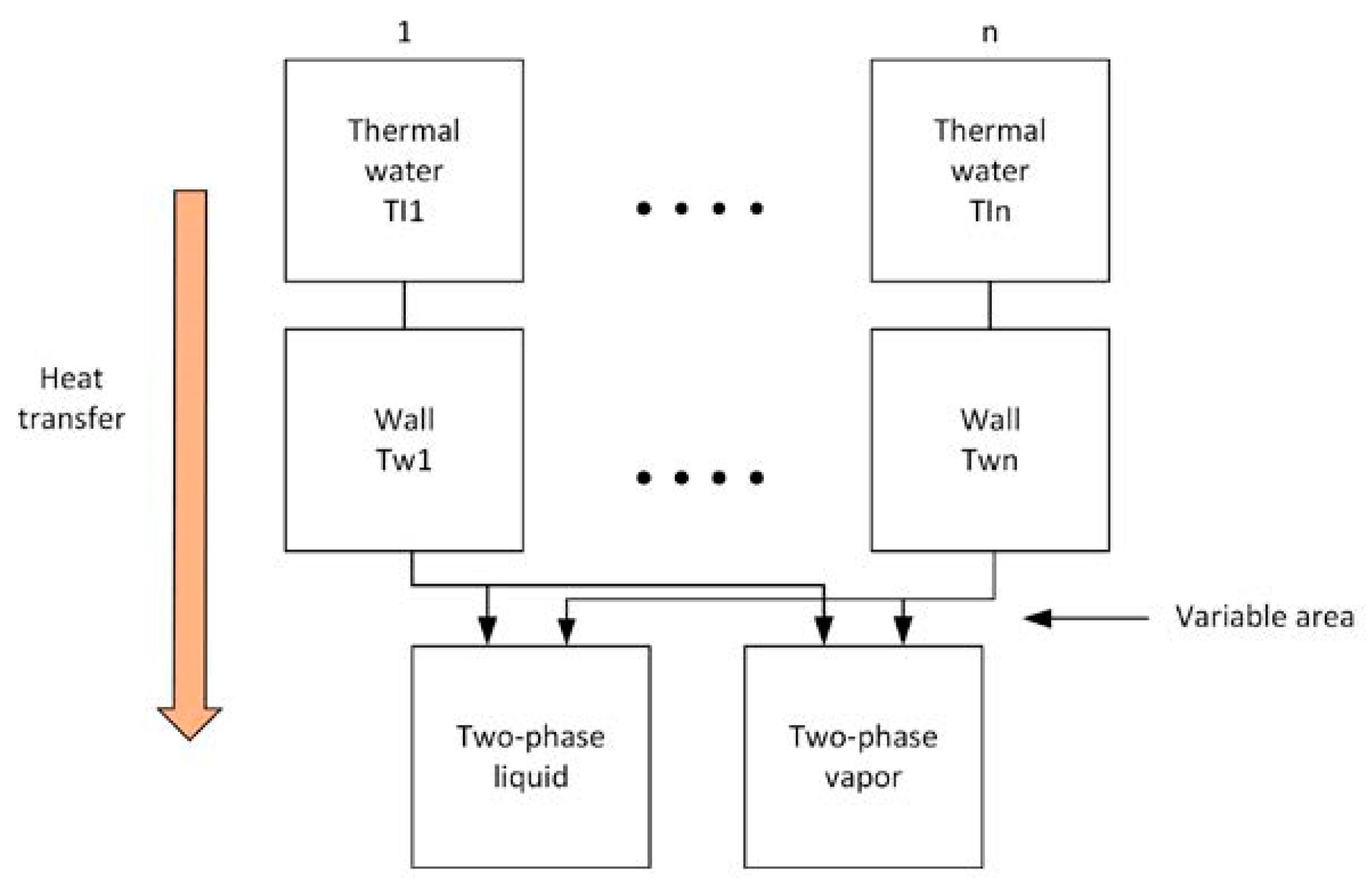
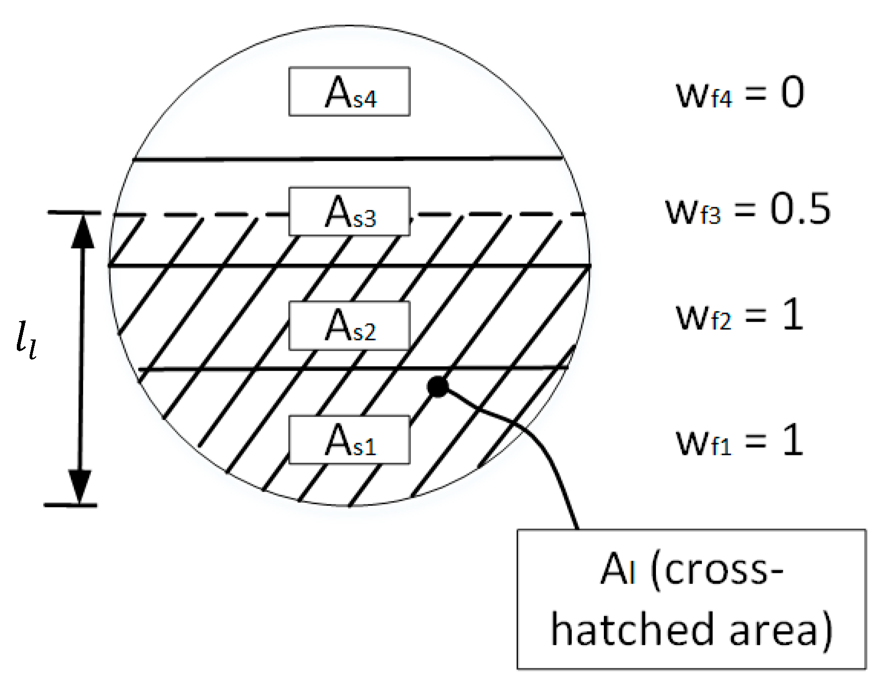
Another modeling approach can be used when a fluid changes phase in a large shell or pool, and the heating/cooling medium flows in a tube bundle. The evaporating/condensing fluid can be represented by means of two volumes (TV) in thermal non-equilibrium. The TV are modelled with a lumped approach, as in the MB model. Unlike the MB model, however, the mass transfer between the TV is a function of the vapor quality in each of the TV, and not a result of the mass and momentum equation at the cell boundaries. As an example, in case of the evaporator, when the vapor quality in the liquid phase is bigger than zero, the liquid is vaporizing, so mass is transferred from the liquid to the vapor region. These mass transfers are independent from the outer direction of flow, which is pressure driven. A TV model for a shell-and-tube condenser is included in the ThermoSysPro library in Modelica
® and discussed in [
65].
An accurate model of the evaporator is essential to reproduce the dynamic behavior of ORC. As an example, most of the control strategies are based on the degree of superheating at the evaporator outlet, or on the evaporation pressure [
41]. The thermal inertia and time response of the evaporator have a crucial impact on how source fluctuations affect the dynamics and control of the power plant. While for small-scale ORC once-through heat exchangers of simple geometry are applied, kettle boilers are very often used in larger scale ORC. Because of the more complex geometry of the kettle, FV and MB cannot represent properly the dynamics of this heat exchanger. In the present work, a dynamic model of a kettle boiler is developed by means of a combination between TV (for the shell-side) and FV method (for the tube/wall side) and validated against measurements from an analogous heat exchanger located in a geothermal power plant in the Munich area. The present work is based on the commercial TIL-Library (Version 3.2.2, TLK-Thermo GmbH, Braunschweig, Germany [
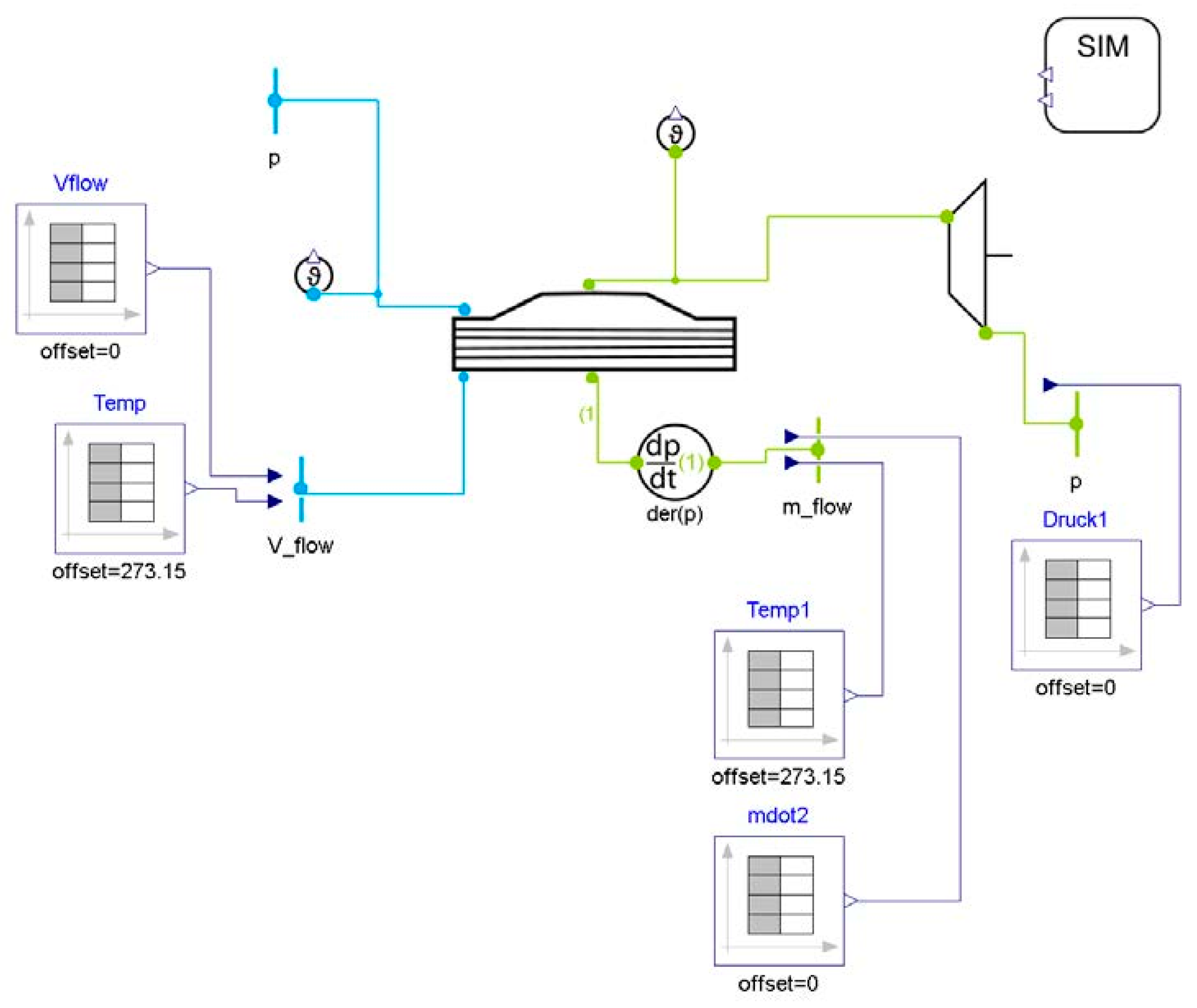
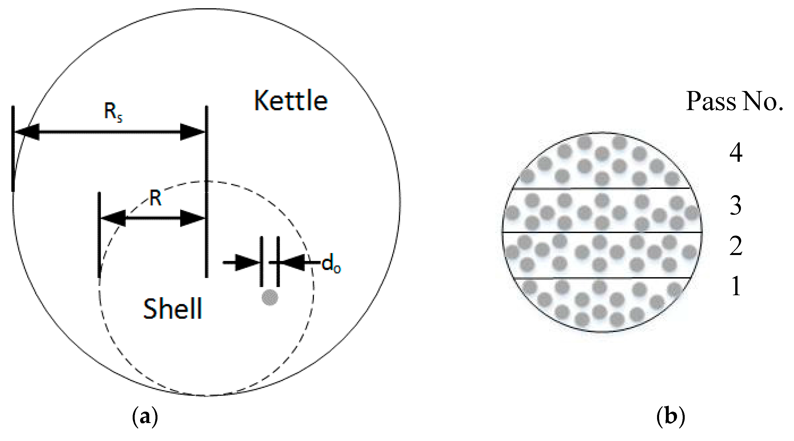
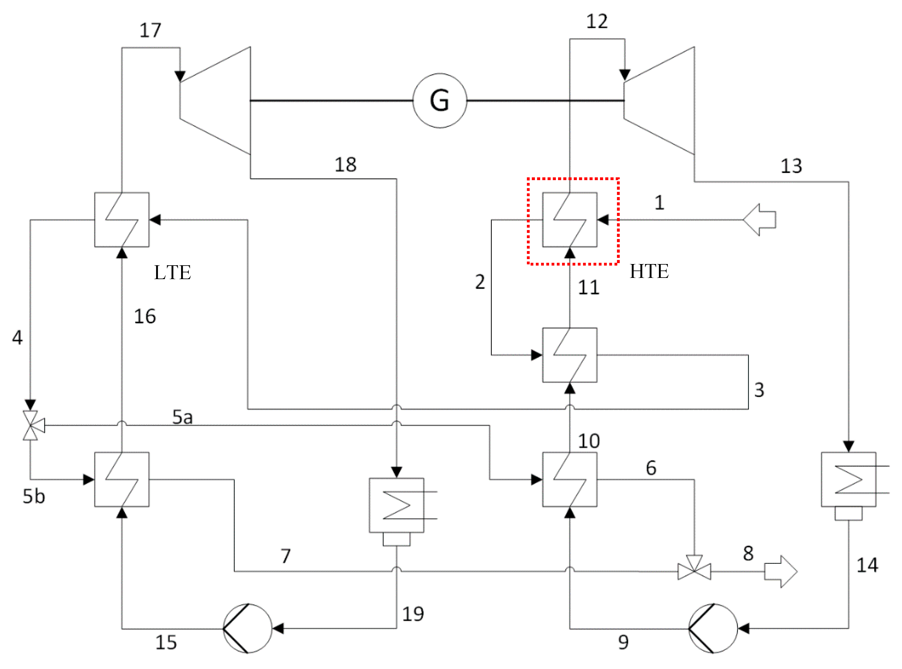
66]). The basic models have been taken from this library, and new components have been developed based on the existing library. The resulting combined TV/FV model can be used for design, off-design and dynamic simulations, and applied for testing and development of basic or advanced control strategies for middle and large-scale ORC power plants.
4. Discussion
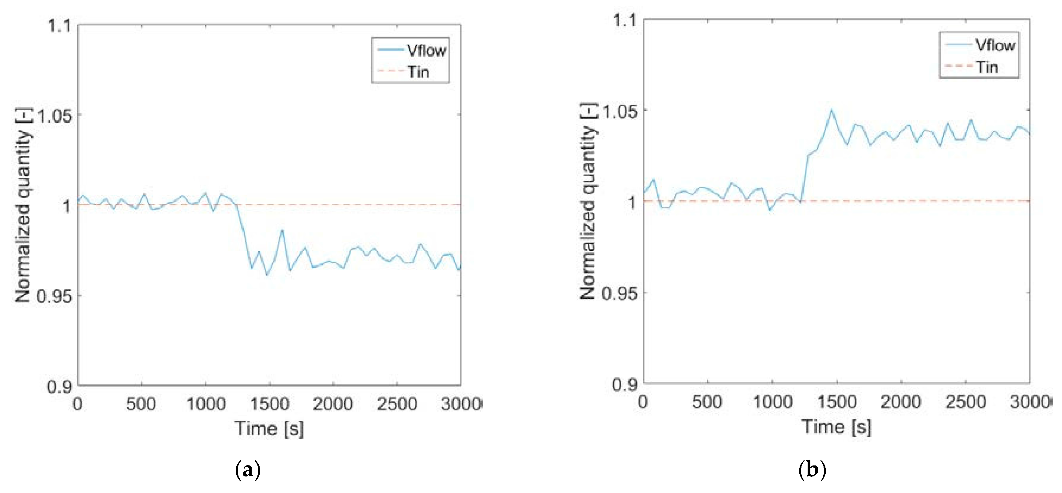
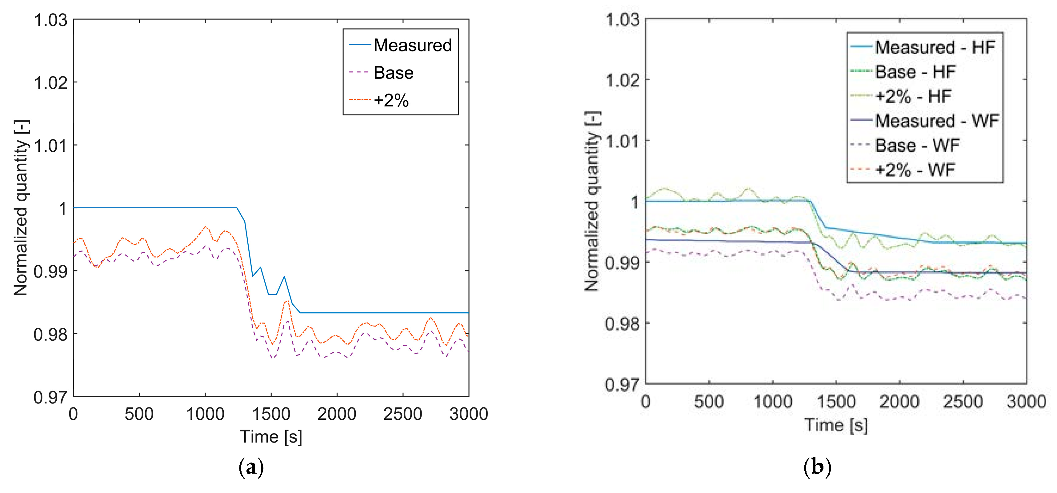
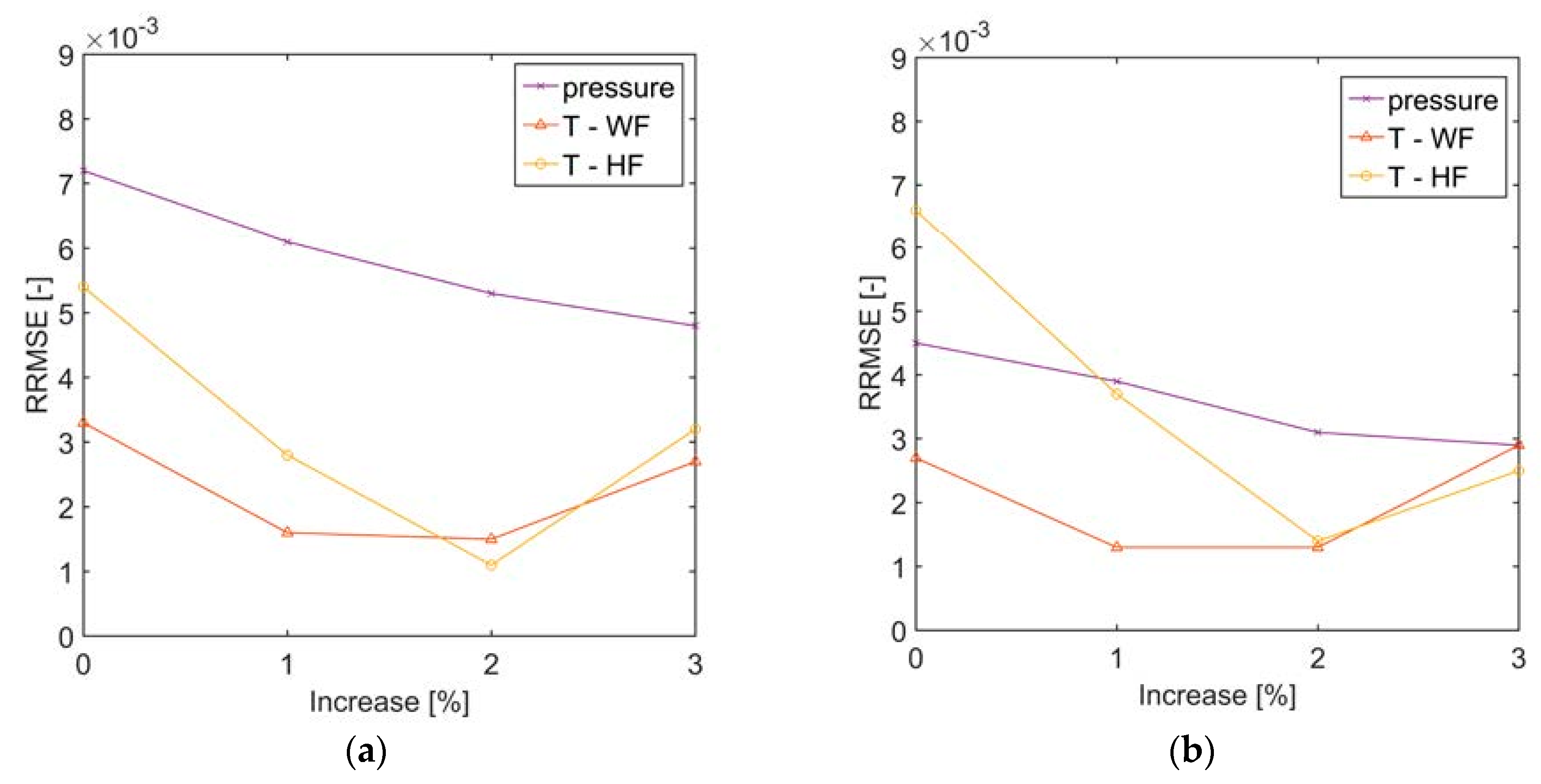
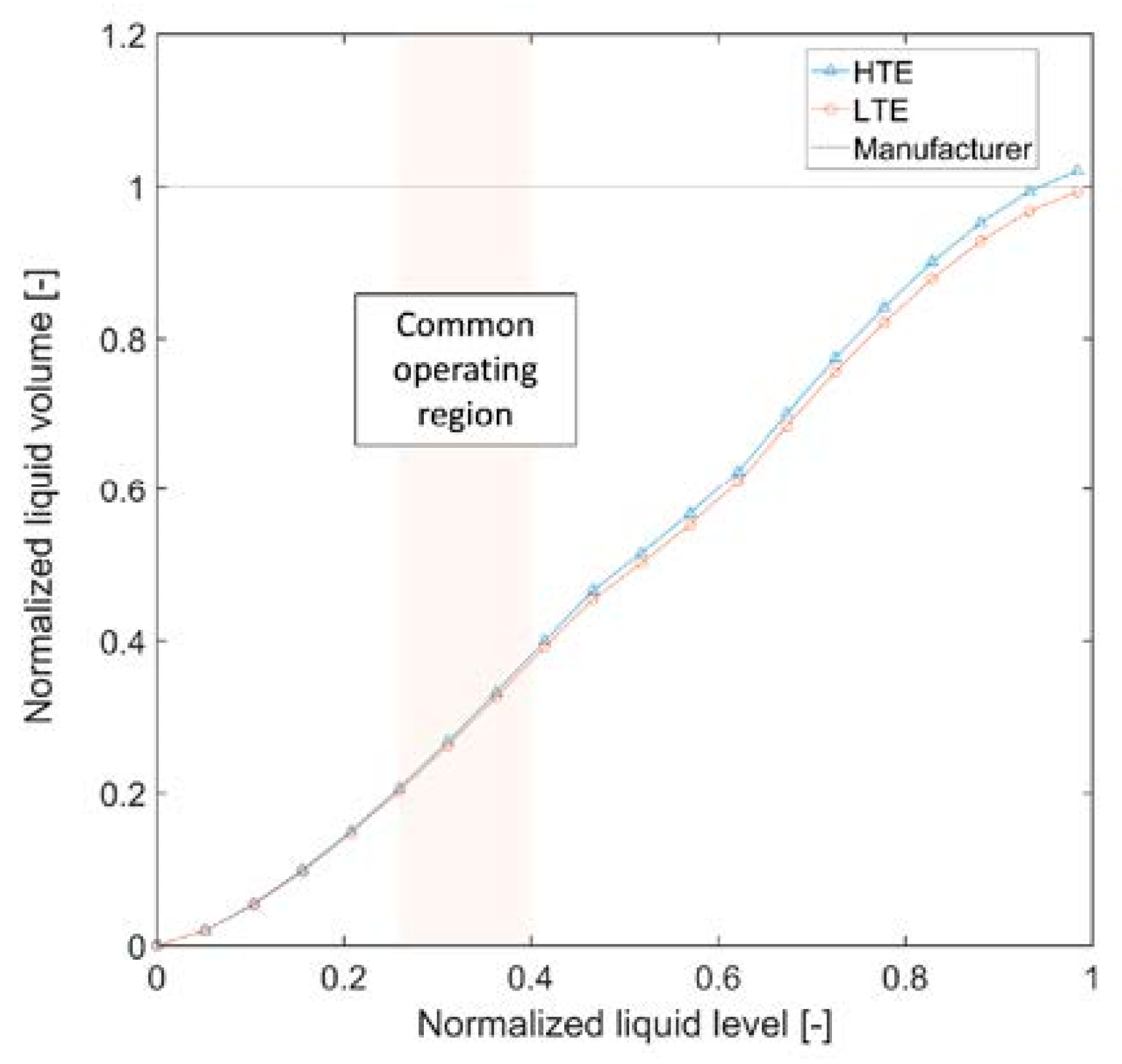
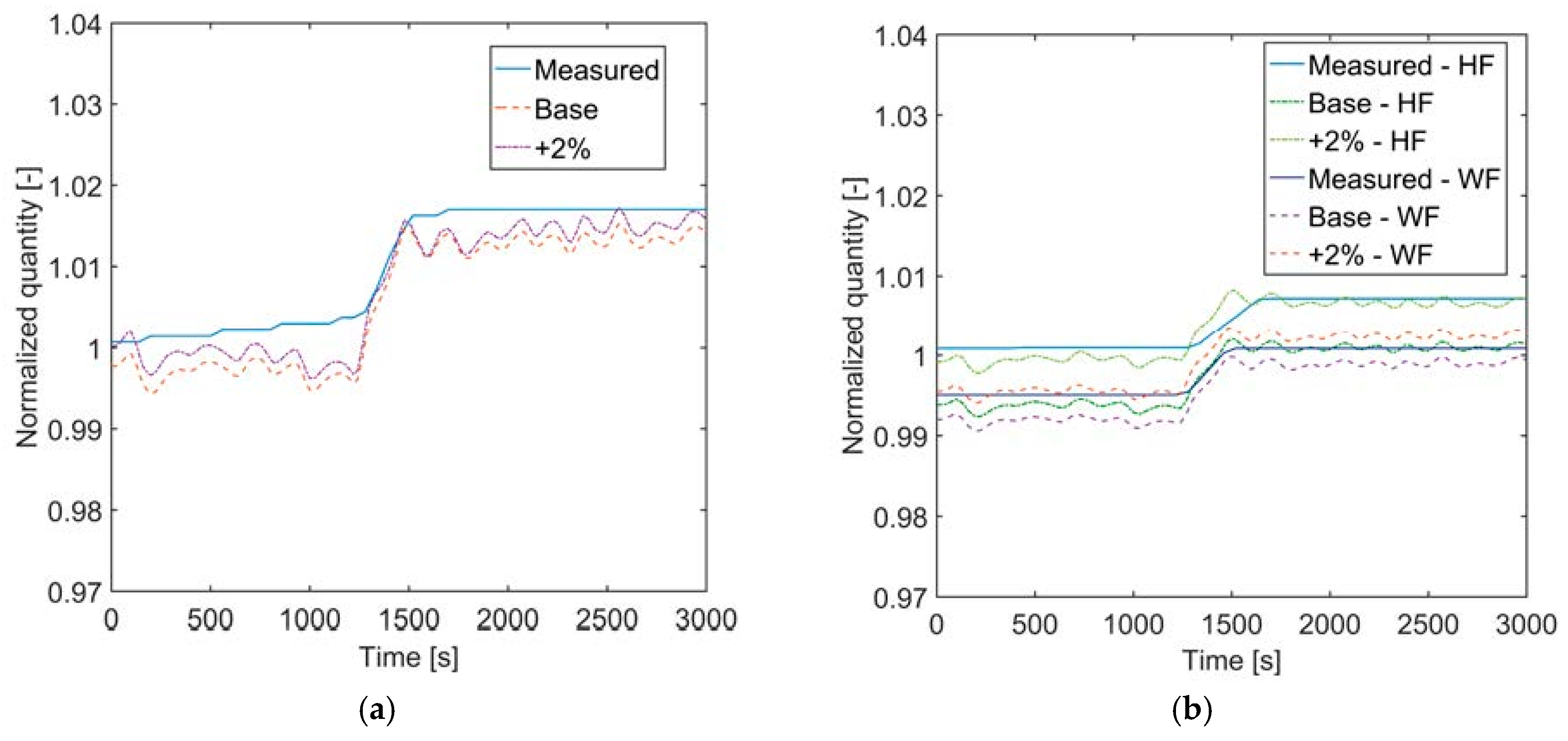
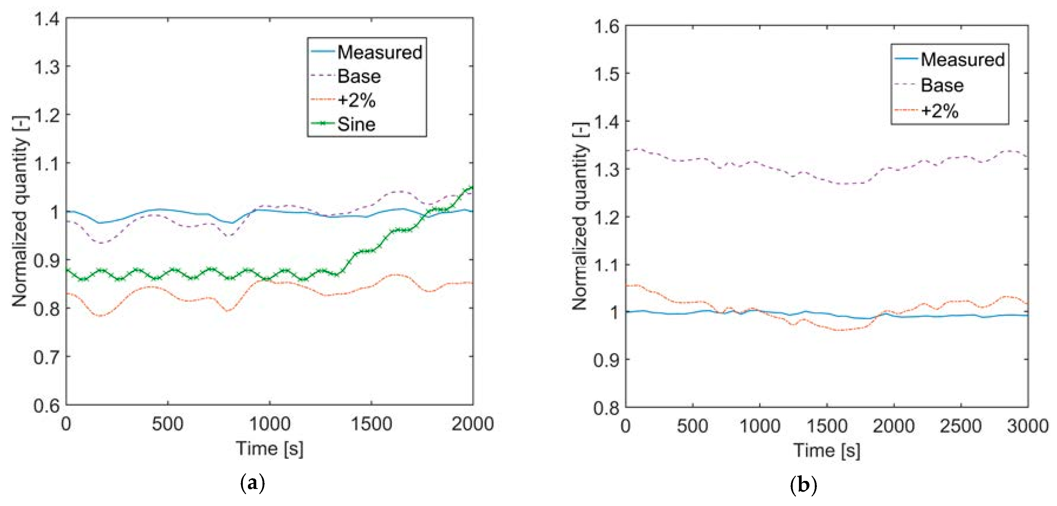
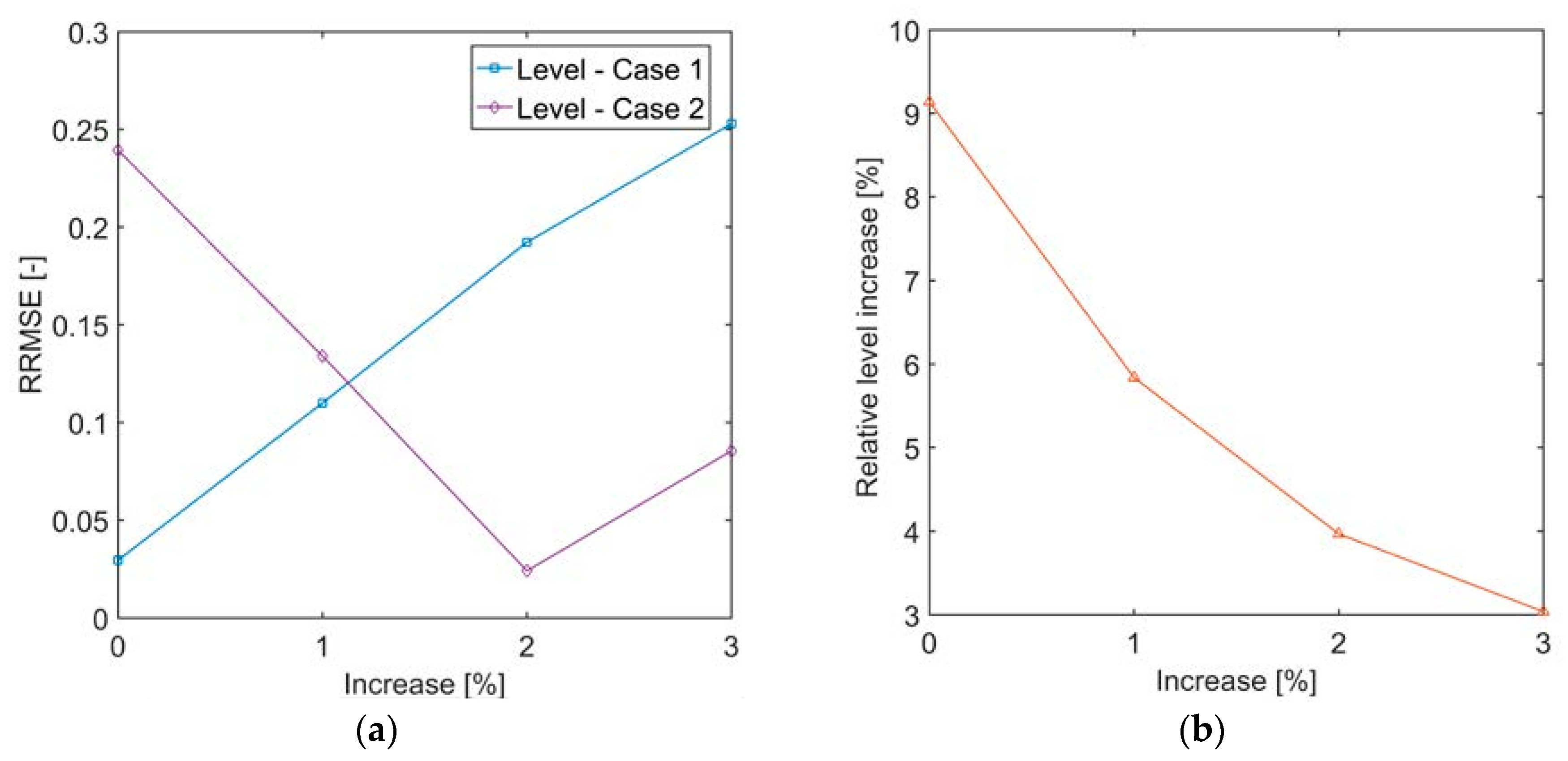
In the present analysis, a dynamic model of a kettle boiler was developed in Modelica® language, by partially making use of models provided by the TIL-library and partially creating new components or features. The boiler model can be effectively useful for larger scale ORC plants, where kettle boilers are very often applied. The model was tested against available measurements from a geothermal CHP plant in Sauerlach, Germany. The pressure of the organic fluid and the outlet temperatures of both organic and heating fluid could be reproduced within a 1% error in case of a negative (Case 1) or positive (Case 2) step change in inlet volume flow rate of the heating fluid.
In
Section 3, the pressure difference between top and bottom of the liquid volume in the evaporator was neglected. The assumption of negligible pressure difference in the liquid level is justified by the fact that the pressure difference is typically below 0.5% of the absolute pressure at the top of the volume. Nevertheless, if such pressure difference is considered, no significant pressure and temperature difference of the vapor is found. The average pressure in the liquid volume would be slightly higher because of the liquid column, and this can lead to a variation of liquid level to 2% with respect to the simplified case. The heat transfer coefficient for pool nucleate boiling (with the Cooper correlation) increases by less than 1%.
The accuracy on the liquid level in the evaporator could not in general be as high as for the evaporator pressure and outlet temperatures. In the attempt to explain the reasons for the liquid level offset (and the improved temperature matching) when increasing the thermal water flow rate by 2% over the entire simulation time, the fluid properties of the thermal water and the working fluid were analyzed, but no clear explanation through these parameters could be found. It might be assumed that the improvement achieved by increasing the volume flow rate of thermal brine could be caused by a deviation in latent heat of vaporization for the working fluid. If the volume flow rate of thermal brine is increased and the amount of working fluid that evaporates does not change, the latent heat of vaporization of the working fluid should be higher in the simulation than in the real case. Using the Peng-Robinson equation instead of REFPROP, the calculated heat of vaporization becomes even smaller, in contrast with the hypothesis. Future work should focus on analyzing the working fluid used in Sauerlach and comparing to the REFPROP database to gain major information on the differences in fluid properties.
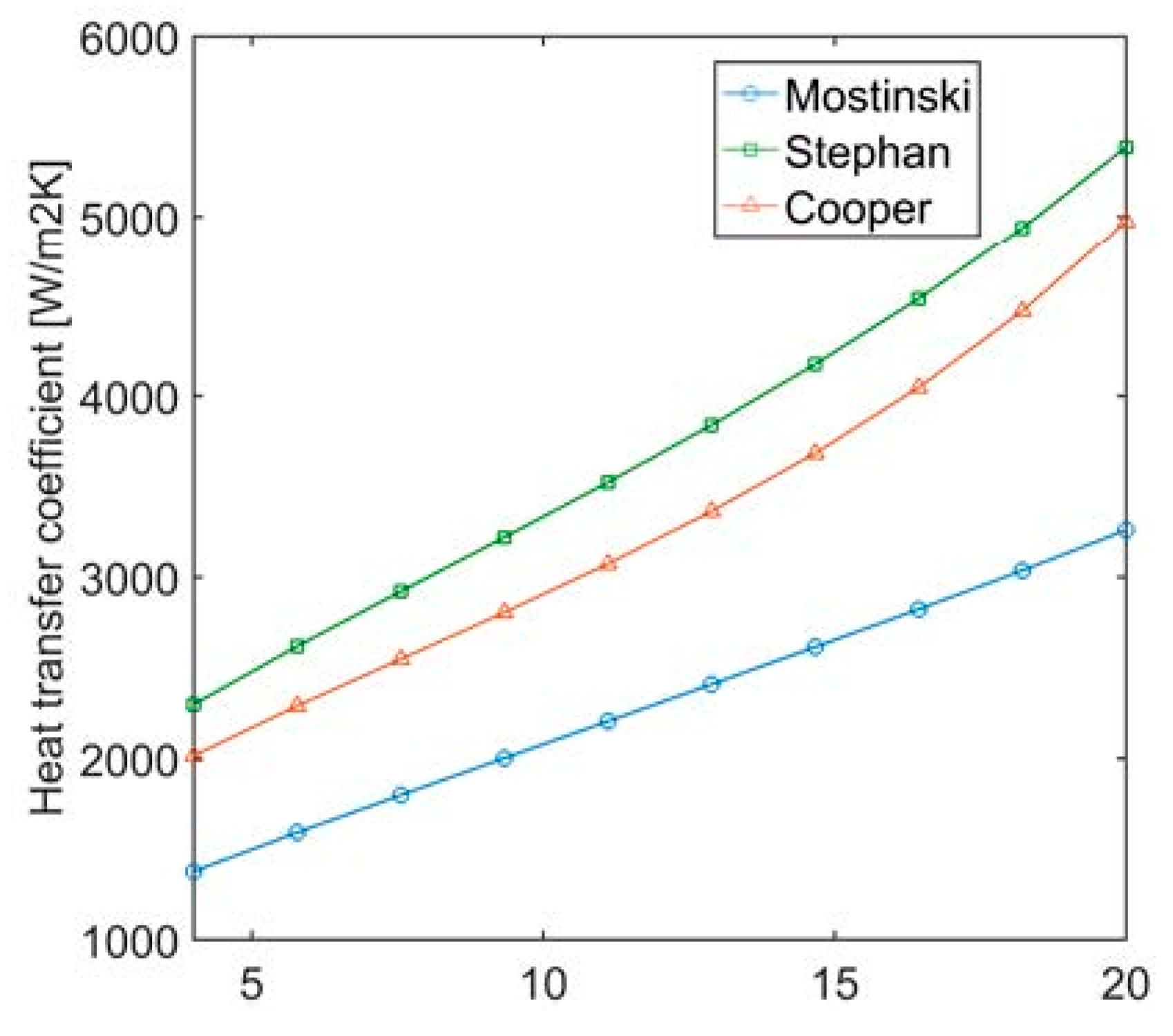
Because of its simplicity and better agreement with the results, the Cooper correlation was used in this work. The Stephan and Mostinski correlations (Equations (23) and (24)) would lead to a higher liquid level because the lower heat transfer coefficient requires a higher heat transfer area to vaporize the same amount of fluid.


