
A Method to Facilitate Uncertainty Analysis in LCAs of Buildings


1
Institute for Sustainable Construction, Edinburgh Napier University, Colinton Road, Edinburgh EH10 5DT, UK
2
Department of Engineering, University of Cambridge, Trumpington Street, Cambridge CB2 1PZ, UK
*
Author to whom correspondence should be addressed.
Energies 2017, 10(4), 524; https://doi.org/10.3390/en10040524
Submission received: 6 March 2017
/
Revised: 6 April 2017
/
Accepted: 11 April 2017
/
Published: 13 April 2017
Abstract
:Life cycle assessment (LCA) is increasingly becoming a common technique to assess the embodied energy and carbon of buildings and their components over their life cycle. However, the vast majority of existing LCAs result in very definite, deterministic values which carry a false sense of certainty and can mislead decisions and judgments. This article tackles the lack of uncertainty analysis in LCAs of buildings by addressing the main causes for not undertaking this important activity. The research uses primary data for embodied energy collected from European manufacturers as a starting point. Such robust datasets are used as inputs for the stochastic modelling of uncertainty through Monte Carlo algorithms. Several groups of random samplings between 101 and 107 are tested under two scenarios: data are normally distributed (empirically verified) and data are uniformly distributed. Results show that the hypothesis on the data no longer influences the results after a high enough number of random samplings (104). This finding holds true both in terms of mean values and standard deviations and is also independent of the size of the life cycle inventory (LCI): it occurs in both large and small datasets. Findings from this research facilitate uncertainty analysis in LCA. By reducing significantly the amount of data necessary to infer information about uncertainty, a more widespread inclusion of uncertainty analysis in LCA can be encouraged in assessments from practitioners and academics alike.
1. Introduction and Theoretical Background
Life cycle assessment (LCA) is a common method whereby the whole life environmental impacts of products can be assessed. Applied within the built environment, the focus is on assessment of products [1], assemblies [2] and whole buildings [3,4], and is predominantly concerned with energy consumption and greenhouse gas emissions [2,4,5]. However, buildings and assemblies are complex entities with long and unpredictable lifespans; they are designed and built by a fragmented industry through temporary and shifting alliances and dispersed supply chains. LCA, therefore, while providing an indication of environmental impacts, includes inherent uncertainties.
It was more than 25 years ago that the US Environmental Protection Agency [6] brought to researchers’ and practitioners’ attention the role and impact of uncertainty and variability in LCA modelling. Nearly ten years has passed since the importance of the topic resurfaced with Lloyd and Ries [7] who revealed a general lack of appreciation of uncertainty modelling and lack of application in life cycle analysis. Even so, almost all life cycle assessment studies in the built environment continue to fail to evaluate the inherent uncertainty [8]. A similar trend has also been observed in civil engineering research [9].
This issue, of course, extends beyond the building sector and affects a significant part of the LCA research and community of practice, but the lack of uncertainty analysis in the LCAs of buildings and building products is particularly severe. Not accounting for uncertainty and variability is important, given that it can severely limit the usefulness of LCA [10], and neglecting uncertainty can have a major impact on the understanding of the problem being analysed, skewing outcomes or misleading decisions based on the analyses [11].
Uncertainty mostly occurs because of the lack of knowledge about the true value (quantity) of a datum [12] but it can also be due to subjective choices [13]. At data level, Huijbregts et al. [14] identified two main issues; data inaccuracy and lack of specific data (further distinguished between data gaps and unrepresentative data). Björklund [12] developed a broad classification of types and sources of uncertainty, these being (1) data inaccuracy; (2) data gaps; (3) unrepresentative data; (4) model uncertainty; (5) uncertainty due to choices; (6) spatial and (7) temporal variability; (8) variability between sources and objects; (9) epistemological uncertainty; (10) mistakes; and (11) estimation of uncertainty. Lloyd and Ries [7] proposed a more concise systemic approach to uncertainty, which can be related to three main elements:
Parameter uncertainty (e.g., the uncertainty refers to the values of a parameter such as the embodied energy or carbon of processes or assemblies); Scenario uncertainty (e.g., the uncertainty refers to the likelihood of different scenarios, such as the UK energy mix in 20 years’ time); Model uncertainty (e.g., the uncertainty refers to the specific model being used, such as the model developed by the IPCC to calculate the global warming potential related to GHGs over 20, 50, and 100 years’ horizons).
Parameter and scenario uncertainty are those considered in LCAs and are often combined with sensitivity analysis to understand the influence of each parameter or scenario towards the final results. In some cases, there seems however to be some confusion between sensitivity and uncertainty analysis and the two terms may be confused as synonyms [15]. Rather, sensitivity analysis is aimed at understanding the influence that input parameters have on the final results whereas uncertainty analysis is aimed at understanding the variability of the final results.
Existing literature on the theoretical foundation of computational structure to undertake uncertainty analysis in LCA is slender [16]. Nonetheless, different techniques exist to analyse uncertainty such as: possibility theory, e.g., [17], fuzzy theory, e.g., [18,19,20], Taylor series expansions, e.g., [21], data quality indicators, e.g., [22,23], expert judgement, e.g., [24,25,26] and practitioners’ belief, e.g., [27] or a combination of two or more techniques, e.g., [28,29]. Despite the breadth of available approaches, uncertainty analysis in built environment LCAs still remains largely untouched.
Stochastic modelling, mainly in the form of Monte Carlo simulation, is the most widely used approach to analyse uncertainty across different products, research areas, and industrial sectors inter alia, [30,31,32,33,34,35,36,37,38,39,40,41]. The usefulness of Monte Carlo simulations relies on the assumption that a sufficient number of trials has been carried out [42] in order to claim something about data distribution and uncertainty. Yet, stochastic modelling and uncertainty analysis can be complicated tasks to undertake, and three main reasons are often found:
It requires more data than is available [36,43,44,45] or is, more generally, too demanding [46]; There is not a definite agreement on the number of iterations that are necessary, which adds to the length (i.e., computational time) and complexity of the calculation [7]; It is perceived as too complex by both academics and practitioners [47]. Work carried out to significantly reduce the required computational power without sacrificing accuracy, e.g., [48], or to compare two classes of error propagation methods, including sampling techniques [49], did not result in a more widespread adoption of Monte Carlo simulation. It therefore remains the case that other methods such as sensitivity and scenario analysis [50,51,52] are more commonly used to quantify uncertainty.
This article intends to complement the knowledge capital already published in the journal on LCAs of buildings by addressing the issues about the amount of data required, the number of iterations, and the complexity of stochastic modelling for uncertainty analysis, offering an innovative solution for the construction sector. The next section introduces the theory and the algorithmic approach developed and used. Results follow, along with a discussion on the wider implication of the findings from this research. The final section concludes the article and presents future work that will be undertaken.
2. Theory and Methods
This research aims to investigate the impact of assumptions on data distribution on the results of uncertainty analysis and to provide an innovative simple approach to reduce the complexity of the assessment and time-consuming data collection activities. It is based on robust primary data collected from European manufacturing plants related to the glass and construction industry [53]. (The quality of the data is demonstrated by the pedigree matrix [22], for the data are characterised by the following scores (2), (2), (1), (2), (1) across the relevant five indicators which are: Reliability, Completeness, Temporal Correlation, Geographical Correlation, Further Technological Correlation—where (1) is the highest possible score and (5) is the lowest, assumed as the default value.) The algorithm has also been tested on randomly generated data and it works equally fine.
The fundamental role of uncertainty analysis in LCAs is easily understood by looking at Figure 1. The figure shows a mock example where the embodied energy (EE) of two alternatives, 1 and 2, are being compared. Most LCAs only provide deterministic, single-valued results which generally represent the most likely values resulting from the specific life cycle inventory (LCI) being considered. These values can be seen as μ1 and μ2 in the figure. If a decision were to be taken only based on such numbers one should conclude that alternative 1 is preferable over alternative 2 since μ1 is lower than μ2. This, unfortunately, is often the case in most existing literature in LCAs of buildings.
However, when considering the relative uncertainty—which provides measures of the standard deviations σ1 and σ2 as well as the probability density function—it is evident that alternative 2 has a far less spread distribution and therefore a much narrower range within which values are likely to vary. This makes, all of sudden, alternative 2 at least as appealing as alternative 1, if not more. The information on uncertainty and data distribution does therefore clearly enable a better and more informed decision making.
In the specific case presented here the processes of the life cycle inventory (LCI) are from the manufacture of one functional unit (FU) of double skin façade, a flat glass cladding systems. In total, 200 items have been followed throughout the supply chain and therefore the dataset available for each entry of the LCI is constituted of 200 data points. For example, cutting the flat glass to the desired measure has been measured and monitored (in terms of energy inputs, outputs, and by-products) for all 200 glass panes and therefore a population of 200 data points is available for that specific process. However, the algorithm presented has been tested successfully also on randomly generated data to ensure its wide applicability. The robust primary data set served the purpose of comparing empirical vs. predicted results.
The data and related life cycle processes refer to embodied energy (MJ or kWh) and embodied carbon (kgCO2e) (for definitions on embodied carbon see, for instance [8]) and both datasets have been used and tested in this research. Embodied energy has however been the main input to the calculation, since embodied carbon is the total carbon dioxide equivalent emissions of embodied energy given the energy mix and carbon conversion factors which are specific to the geographical context under consideration. Therefore, to avoid duplication of figures, only embodied energy results have been included in the article.
Figure 2 shows the specific embodied energy of three such processes against the frequency with which they occur.
The graphs in the figure present the cumulative distribution function (CDF) of the collected data plotted against the CDF of the data if they were perfectly normally distributed. The check on the approximation of the real distribution of the dataset versus a normal distribution has been conducted through the Z-test [54]. As the plots in the figure show, there is good agreement between the collected data and normally distributed data, and therefore the hypothesis that the collected data were normally distributed was adopted.
The primary data collection represented a time-consuming and costly activity. Therefore, the research team wondered whether it was possible to infer information on the uncertainty of the result of the LCA as well as its probability distribution without embarking onto such an extensive data collection. To do so, the empirical case of collected primary data characterised by a normal distribution has been used as a reference. This was then compared with a less demanding approach to determine variability in the data. The simplest alternative is generally the use of a maximum–minimum variation range, whereby the only known piece of information is that a value is likely to vary within that range. The likelihood of different values within that range remains, however, unknown. From a probabilistic point of view, the closest case to this maximum–minimum scenario is that of a uniform distribution, which is characterised by a defined data variation range within which all values have the same probability. The comparison between these two alternatives, and their influence on the uncertainty of the result of the LCA, was the underpinning idea for this research. This has been tested through the algorithm developed and explained in detail in the next section.
The Algorithm Developed for This Research
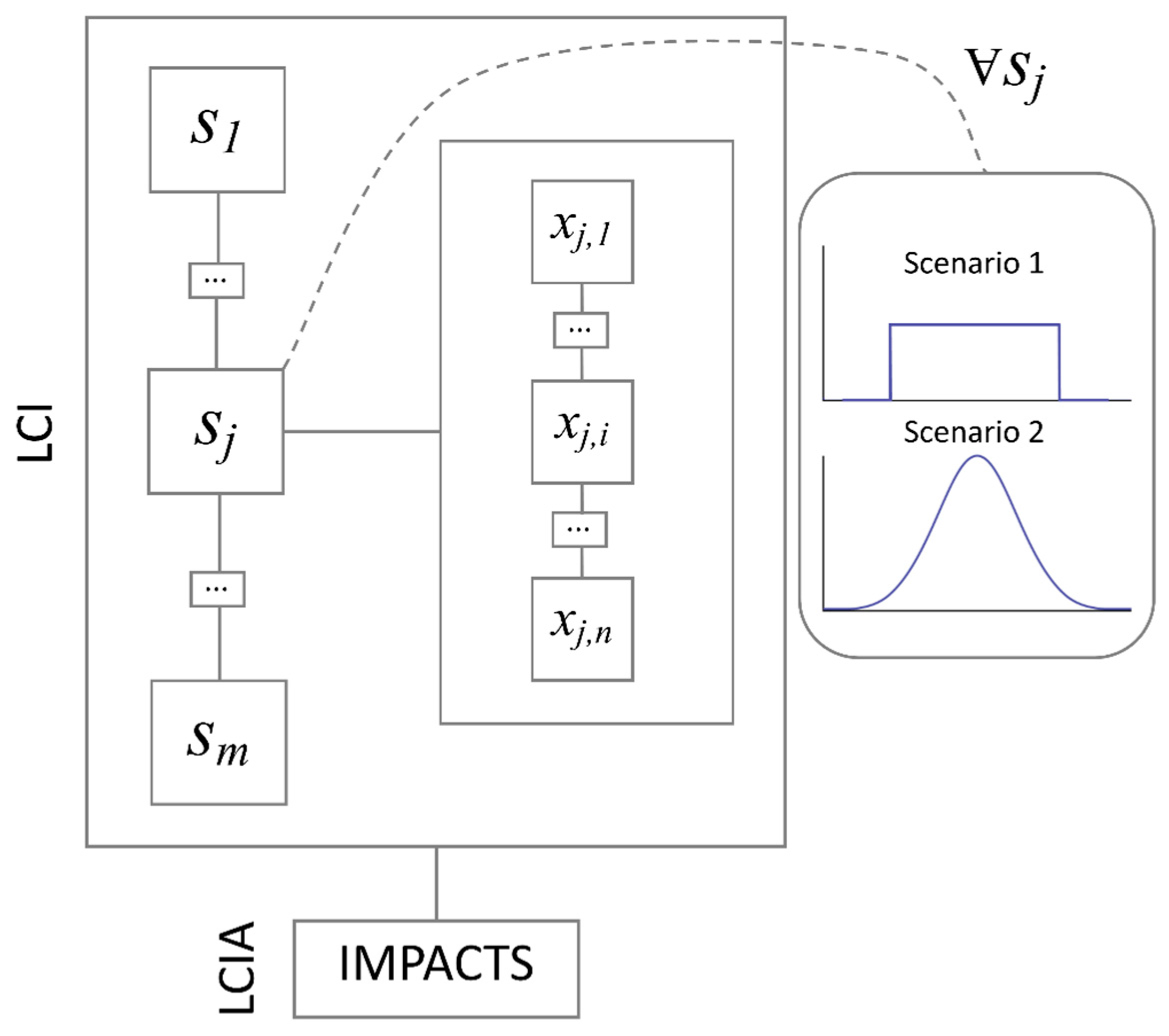
To explain the algorithm, let us assume the life cycle inventory (LCI) of the primary data collection is arranged as a vector P:
with m representing the total number of sub-processes and the jth entry being, in turn, another vector s, containing the entire dataset of n measures of embodied energy, x, associated with the jth manufacturing sub-process:
In order to perform a Monte Carlo analysis, an input domain is required from which xi variables can be randomly picked according to a given probability distribution. For each j sub-process, two sets of continuous input domains are derived in here from the discrete data collection P. Namely: a vector N containing n pairs of values μj and σj, representing respectively the mean and standard deviation of xi values of embodied energy associated with the jth sub-process.
where,
as well as a vector U containing n pairs of values xj,min and xj,max, representing respectively the minimum and maximum embodied energy values, xi, associated with the jth sub-process:
Two sets of Monte Carlo simulations were then run, each with a prescribed increasing number of output samples to be generated (i.e., from 101 to 107). The inputs for the first set were randomly sampled, under the assumption that data were normally distributed (as from N), from a probability density function defined as:
whereas the assumption of uniform distribution (as from U) was used for the second set, and data were randomly sampled from a probability density function defined as:
As explained, the normal distribution was the distribution that best fitted the primary data collected, whereas the uniform distribution was chosen because it is characterised by the lowest number of required inputs where only the lower and upper bounds of the variation range are necessary. As such, it represents the least intensive option in terms of data collection to enable an uncertainty analysis.
The single output obtained at the end of each Monte Carlo iteration is a summation of the (randomly picked) embodied energy values, x, associated with the jth sub-process. This represents an estimate of the embodied energy associated with the LCI, which is in this case the entire manufacturing process. This is because, mathematically, a life cycle impact assessment (LCIA) equals to:
which represents the summation of the impacts of the jth process S across the life cycle inventory P for the relevant impact category being considered (e.g., cumulative energy demand).
The algorithmic approach is also shown visually in Figure 3.
As mentioned, the collection of data to characterise the data distribution is a significantly time-consuming and costly activity, which often severely limits or completely impedes undertaking uncertainty analysis [46]. The literature reviewed has shown that different approaches arose as alternative, more practical solutions. Out of those, one of the most often utilised in practice in the construction industry is the use of expert judgement to identify a range within which data is expected to vary [24,25]. This is then repeated for several or indeed all life cycle processes that constitute the life cycle inventory and it generally leads to calculating a minimum and maximum value for the overall impact assessment, which are then labelled as ‘worst’ and ‘best’ case scenario.
It has been shown that expert judgements can provide an accurate overview of the variability range [26], and this characteristic held true in the case of the research underpinning this article. Practitioners and professionals involved in the life cycle processes for which primary data have been collected have indeed shown a remarkably accurate sensitivity to the processes variation range. As a result, it would have been possible to identify the same (or significantly similar) data range, which resulted from the extensive data collection by asking people in the industry: “What are the best and worst case scenarios in terms of energy input for this specific process?” However, the answer to such a question tells nothing about the way data are distributed between these scenarios, and both values represent the least probable events, as they are, statistically speaking, the farthest points from the mean (i.e., most likely value). If this approach were propagated throughout the whole LCI, the result would lead to an overall range for the impact assessment which is characterised by significant confidence in terms of inclusion of the true value but the numbers it produces would likely be of very little use. As a consequence, the resulting decisions could be significantly biased, with the risk of invalidating the merit and efforts of the whole LCA [10].
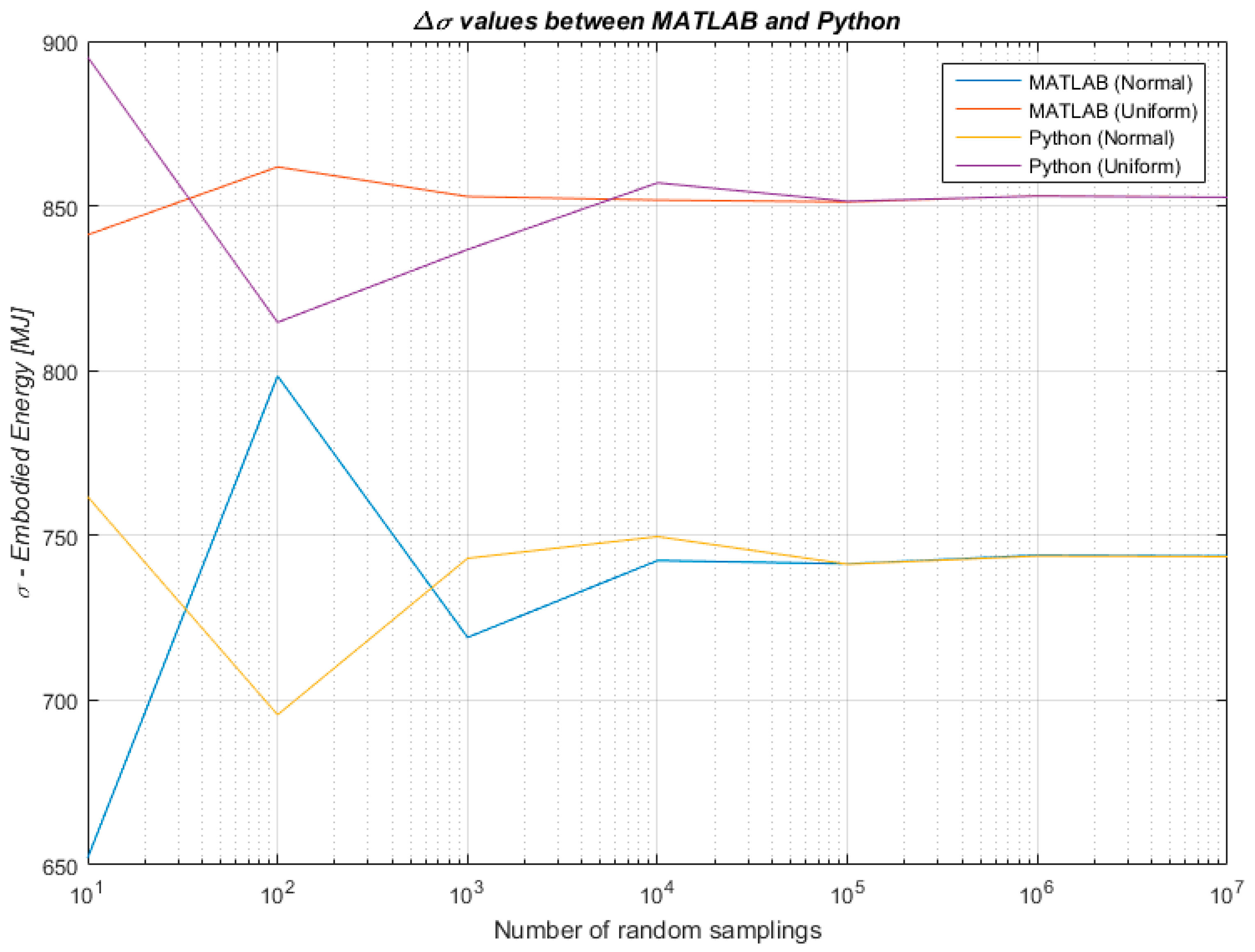
Therefore, to combine the benefits of a lighter data collection with the benefit of an uncertainty analysis, the algorithmic approach developed for this research has tested whether and to what extent the knowledge of a data distribution within a known data variation range influences the outcome of an uncertainty analysis undertaken through Monte Carlo simulation. The algorithmic approach has been developed, implemented and tested in MATLAB R2015b (8.6.0). Once initial results were obtained, the robustness of the findings has been further tested for validity by one of the co-authors who independently implemented an algorithm in Python with the aim of addressing the same research problem. Findings were therefore confirmed across the two programming languages with different algorithms written by two of the authors to strengthen the reliability of our results. A comparison of the results produced in MATLAB and Python 3.5 is shown in Figure 4 and Figure 5 for the mean values µ and the standard deviations σ respectively.
To broaden the impact and applicability of the approach developed, and to strengthen the relevance of its findings, two extreme cases have been tested:
- LCI is constituted by as few as two entries (e.g., only two life cycle processes)—an example could be a very simple construction product or material such as unfired clay;
- LCI is constituted by as many entries as those for which collected primary data were available.
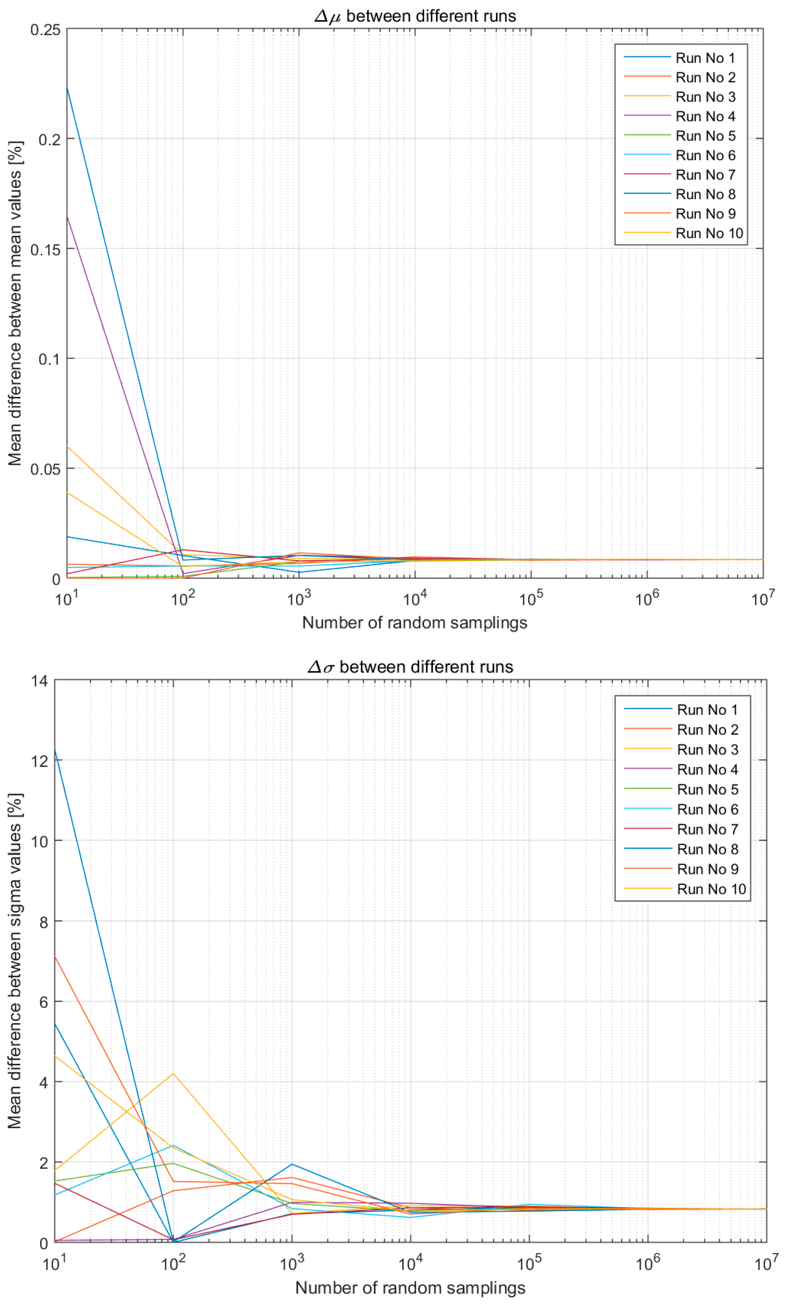
In terms of number of samplings and iterations, each run of the Monte Carlo algorithm randomly and iteratively samples 10i (with i = 1, …, 7 and 10i+1 step increases) values from within each range under the pertinent assumption regarding data distribution (that is, uniform in one case and normal in the other). This process repeats across all entries of the LCI and produces the final figures for the impact assessment. The random sampling mechanism is not pre-assigned or registered, and it varies at each and new run of the algorithm. The algorithm stops after 10 different runs, a high enough number to ensure that potential biases in the variability with which the random sampling operates would emerge.
3. Results and Discussion
Figure 6 shows the results for one specific run out of the ten the algorithm runs for both hypotheses on data distribution: uniform (S1) and normal (S2).
The histograms refer to the LCIA (overall impact) and not to the LCI (individual inputs). All seven sampling cases are shown, from 101 to 107 random samplings. The figures show that for lower numbers of samplings the characteristics of the two distributions are still evident whereas from 104 random samples upwards the results of the two methods converge. The algorithm calculates also the difference between the mean values and standard deviations and normalises them to a percentage. This information is presented in the last (bottom-right) graph of Figure 6. It can be seen how the difference between μ and σ under the two hypotheses is not influential anymore after 103–104 samplings. If for the mean this could be expected as a consequence of the central limit theorem, this finding is noteworthy for the standard deviation.
Figure 7 shows the μ and σ variation (percentage) between the two hypotheses across all 10 runs in the case of a simplistic LCI composed of two entries. In all runs, regardless of the initial difference for lower number of samplings, after 105 random samplings the average differences stabilise around:
- 0.01% for the μ, and,
- 1% for the σ.
Figure 8 presents the same results but for the full LCI as explained in the research design section. In the case of the detailed LCI, after 104 random samplings the average differences stabilise around:
- 0.01% for the μ, and,
- 1% for the σ.
This demonstrates the validity of the approach developed regardless of the size of the LCI (i.e., number of entries from which the algorithm samples randomly). It should be noted that despite it takes 105 samplings to achieve perfect convergence in the case of an LCI made of just two entries, the stabilisation of any variation around 0.01% for the μ and 1% for the σ is already clearly identifiable from 104 samplings.
In terms of computational costs, the algorithm is extremely light and the whole lot of 10 runs, each of which has seven iterations, from 101 to 107 random samplings, only takes 61.594 s to run in the case of the full LCI on a MacBook Pro. Specifically, the core computations take 38 s.
To ensure that the LCI with as little as two entries would be representative of a generic case and not just of a fortunate combination of two processes that confirm the general case, we have further tested this simplified inventory through five combinations of two processes randomly picked from the database. These have been tested again on both embodied energy and embodied carbon data, and graphical results for the embodied carbon in all five cases are provided as supplementary material attached to this article (Figures S1–S5).
These findings address current challenges in uncertainty analysis in LCA as described in the introduction, and have implications for both theory and practice. Firstly, it has been shown that extensive data collection to characterise the data distribution is not necessary to undertake an uncertainty analysis. As few as two numbers (the upper and lower bounds of the data variation range) combined with a sensible use of the power of Monte Carlo simulation suffice to characterise and propagate uncertainty. Secondly, it has also been found that 104 random samplings are sufficient to achieve convergence, thus establishing a reference number for random samplings within Monte Carlo simulation, at least for uncertainty analysis from LCIs similar to the one in question, i.e., built environment studies. Thirdly, the high computational costs often associated with Monte Carlo simulation have been reduced, through the simple and innovative algorithm developed.
4. Conclusions and Future Work
The research presented in this article has addressed current challenges in uncertainty analysis in LCA of buildings. By means of an innovative approach based on Monte Carlo simulation, it has tested the influence of two different assumptions on data distribution towards the final results of the uncertainty analysis. The different assumptions on the data sets tested in this research were (1) data with a normal distribution and (2) data with a uniform distribution, both based on primary data collected as part of a robust dataset. Results have demonstrated that after 104 random samplings from within the data variation range, the initial assumption on whether the data were normally or uniformly distributed loses relevance, both in terms of mean values and standard deviations.
The consequence of the findings is that an initial characterisation and propagation of uncertainty within a life cycle inventory during an LCA of buildings can be carried out without the usually expensive and time consuming primary data collection. The approach presented here therefore allows a simplified way to include uncertainty analysis within the LCA of complex construction products, assemblies and whole buildings. In turn, this should encourage increased confidence in, and therefore increased uptake of, the LCA calculation in the construction industry, leading eventually to meaningful and reliable reduction of environmental impacts.
Future work will test the influence of more data distributions used and found in LCA practice in the built environment, including triangular, trapezoidal, lognormal, and beta distributions. In its current form the approach developed requires the use of MATLAB, which could be a limit to its widespread adoption. As a consequence, we intend to develop a web-based free application hosted on an academic website where academics and practitioners alike can update their data as Excel or .csv files and get results in both graphical and datasheet formats. In the meantime, interested users are encouraged to contact the authors to find out more about the algorithm or to have their LCI data processed for uncertainty analysis.
Supplementary Materials
The following are available online at www.mdpi.com/1996-1073/10/4/524/s1, Figures S1–S5: μ and σ variation (percentage) between the two hypotheses across 5 runs (for 5 random combinations of two LCI entries).
Acknowledgments
Funding for this research was received from EPSRC (Award Ref. EP/N509024/1) and the Isaac Newton Trust (RG74916). The authors are grateful to William Fawcett and Martin Hughes who listened to the ideas behind this research and provided useful and constructive feedback as well as positive and encouraging comments. Grateful thanks are also extended to the reviewers for their inputs and comments throughout the review process.
Author Contributions
Francesco Pomponi collected the primary data, conceived and designed the research, and wrote the algorithm in MATLAB; Bernardino D’Amico wrote the algorithm in Python to validate the research findings; all authors contributed to multiple drafts that gave the article its present form.
Conflicts of Interest
The authors declare no conflict of interest.
References
- Neri, E.; Cespi, D.; Setti, L.; Gombi, E.; Bernardi, E.; Vassura, I.; Passarini, F. Biomass Residues to Renewable Energy: A Life Cycle Perspective Applied at a Local Scale. Energies 2016, 9, 922. [Google Scholar] [CrossRef]
- Bonamente, E.; Cotana, F. Carbon and Energy Footprints of Prefabricated Industrial Buildings: A Systematic Life Cycle Assessment Analysis. Energies 2015, 8, 12685–12701. [Google Scholar] [CrossRef]
- Thiel, C.; Campion, N.; Landis, A.; Jones, A.; Schaefer, L.; Bilec, M. A Materials Life Cycle Assessment of a Net-Zero Energy Building. Energies 2013, 6, 1125–1141. [Google Scholar] [CrossRef]
- Zabalza, I.; Scarpellini, S.; Aranda, A.; Llera, E.; Jáñez, A. Use of LCA as a Tool for Building Ecodesign. A Case Study of a Low Energy Building in Spain. Energies 2013, 6, 3901–3921. [Google Scholar] [CrossRef]
- Magrassi, F.; Del Borghi, A.; Gallo, M.; Strazza, C.; Robba, M. Optimal Planning of Sustainable Buildings: Integration of Life Cycle Assessment and Optimization in a Decision Support System (DSS). Energies 2016, 9, 490. [Google Scholar] [CrossRef]
- United States Environmental Protection Agency (US EPA). Exposure Factors Handbook; Report EPA/600/8-89/043; United States Enviornmental Protection Agency: Washington, DC, USA, 1989.
- Lloyd, S.M.; Ries, R. Characterizing, Propagating, and Analyzing Uncertainty in Life-Cycle Assessment: A Survey of Quantitative Approaches. J. Ind. Ecol. 2007, 11, 161–179. [Google Scholar] [CrossRef]
- Pomponi, F.; Moncaster, A.M. Embodied carbon mitigation and reduction in the built environment—What does the evidence say? J. Environ. Manag. 2016, 181, 687–700. [Google Scholar] [CrossRef] [PubMed]
- Zhang, Y.-R.; Wu, W.-J.; Wang, Y.-F. Bridge life cycle assessment with data uncertainty. Int. J. Life Cycle Assess. 2016, 21, 569–576. [Google Scholar] [CrossRef]
- Huijbregts, M. Uncertainty and variability in environmental life-cycle assessment. Int. J. Life Cycle Assess. 2002, 7, 173. [Google Scholar] [CrossRef]
- Di Maria, F.; Micale, C.; Contini, S. A novel approach for uncertainty propagation applied to two different bio-waste management options. Int. J. Life Cycle Assess. 2016, 21, 1529–1537. [Google Scholar] [CrossRef]
- Björklund, A.E. Survey of approaches to improve reliability in LCA. Int. J. Life Cycle Assess. 2002, 7, 64–72. [Google Scholar] [CrossRef]
- Cellura, M.; Longo, S.; Mistretta, M. Sensitivity analysis to quantify uncertainty in Life Cycle Assessment: The case study of an Italian tile. Rene. Sustain. Energy Rev. 2011, 15, 4697–4705. [Google Scholar] [CrossRef]
- Huijbregts, M.A.J.; Norris, G.; Bretz, R.; Ciroth, A.; Maurice, B.; Bahr, B.; Weidema, B.; Beaufort, A.S.H. Framework for modelling data uncertainty in life cycle inventories. Int. J. Life Cycle Assess. 2001, 6, 127–132. [Google Scholar] [CrossRef]
- Roeder, M.; Whittaker, C.; Thornley, P. How certain are greenhouse gas reductions from bioenergy? Life cycle assessment and uncertainty analysis of wood pellet-to-electricity supply chains from forest residues. Biomass Bioenergy 2015, 79, 50–63. [Google Scholar] [CrossRef]
- Heijungs, R.; Suh, S. The Computational Structure of Life Cycle Assessment; Springer Science & Business Media: New York, NY, USA, 2002; Volume 11. [Google Scholar]
- André, J.C.S.; Lopes, D.R. On the use of possibility theory in uncertainty analysis of life cycle inventory. Int. J. Life Cycle Assess. 2011, 17, 350–361. [Google Scholar] [CrossRef]
- Benetto, E.; Dujet, C.; Rousseaux, P. Integrating fuzzy multicriteria analysis and uncertainty evaluation in life cycle assessment. Environ. Model. Softw. 2008, 23, 1461–1467. [Google Scholar] [CrossRef]
- Heijungs, R.; Tan, R.R. Rigorous proof of fuzzy error propagation with matrix-based LCI. Int. J. Life Cycle Assess. 2010, 15, 1014–1019. [Google Scholar] [CrossRef]
- Egilmez, G.; Gumus, S.; Kucukvar, M.; Tatari, O. A fuzzy data envelopment analysis framework for dealing with uncertainty impacts of input–output life cycle assessment models on eco-efficiency assessment. J. Clean. Prod. 2016, 129, 622–636. [Google Scholar] [CrossRef]
- Hoxha, E.; Habert, G.; Chevalier, J.; Bazzana, M.; Le Roy, R. Method to analyse the contribution of material's sensitivity in buildings’ environmental impact. J. Clean. Prod. 2014, 66, 54–64. [Google Scholar] [CrossRef]
- Weidema, B.P.; Wesnæs, M.S. Data quality management for life cycle inventories—An example of using data quality indicators. J. Clean. Prod. 1996, 4, 167–174. [Google Scholar] [CrossRef]
- Wang, E.; Shen, Z. A hybrid Data Quality Indicator and statistical method for improving uncertainty analysis in LCA of complex system—Application to the whole-building embodied energy analysis. J. Clean. Prod. 2013, 43, 166–173. [Google Scholar] [CrossRef]
- Sonnemann, G.W.; Schuhmacher, M.; Castells, F. Uncertainty assessment by a Monte Carlo simulation in a life cycle inventory of electricity produced by a waste incinerator. J. Clean. Prod. 2003, 11, 279–292. [Google Scholar] [CrossRef]
- Von Bahr, B.; Steen, B. Reducing epistemological uncertainty in life cycle inventory. J. Clean. Prod. 2004, 12, 369–388. [Google Scholar] [CrossRef]
- Lasvaux, S.; Schiopu, N.; Habert, G.; Chevalier, J.; Peuportier, B. Influence of simplification of life cycle inventories on the accuracy of impact assessment: Application to construction products. J. Clean. Prod. 2014, 79, 142–151. [Google Scholar] [CrossRef]
- Benetto, E.; Dujet, C.; Rousseaux, P. Possibility Theory: A New Approach to Uncertainty Analysis? (3 pp). Int. J. Life Cycle Assess. 2005, 11, 114–116. [Google Scholar] [CrossRef]
- Coulon, R.; Camobreco, V.; Teulon, H.; Besnainou, J. Data quality and uncertainty in LCI. Int. J. Life Cycle Assess. 1997, 2, 178–182. [Google Scholar] [CrossRef]
- Lo, S.-C.; Ma, H.-W.; Lo, S.-L. Quantifying and reducing uncertainty in life cycle assessment using the Bayesian Monte Carlo method. Sci. Total Environ. 2005, 340, 23–33. [Google Scholar] [CrossRef] [PubMed]
- Bojacá, C.R.; Schrevens, E. Parameter uncertainty in LCA: Stochastic sampling under correlation. Int. J. Life Cycle Assess. 2010, 15, 238–246. [Google Scholar] [CrossRef]
- Canter, K.G.; Kennedy, D.J.; Montgomery, D.C.; Keats, J.B.; Carlyle, W.M. Screening stochastic life cycle assessment inventory models. Int. J. Life Cycle Assess. 2002, 7, 18–26. [Google Scholar] [CrossRef]
- Ciroth, A.; Fleischer, G.; Steinbach, J. Uncertainty calculation in life cycle assessments. Int. J. Life Cycle Assess. 2004, 9, 216–226. [Google Scholar] [CrossRef]
- Geisler, G.; Hellweg, S.; Hungerbuhler, K. Uncertainty analysis in life cycle assessment (LCA): Case study on plant-protection products and implications for decision making. Int. J. Life Cycle Assess. 2005, 10, 184–192. [Google Scholar] [CrossRef]
- Huijbregts, M.A.J. Application of uncertainty and variability in LCA. Int. J. Life Cycle Assess. 1998, 3, 273–280. [Google Scholar] [CrossRef]
- Huijbregts, M.A.J. Part II: Dealing with parameter uncertainty and uncertainty due to choices in life cycle assessment. Int. J. Life Cycle Assess. 1998, 3, 343–351. [Google Scholar] [CrossRef]
- Miller, S.A.; Moysey, S.; Sharp, B.; Alfaro, J. A Stochastic Approach to Model Dynamic Systems in Life Cycle Assessment. J. Ind. Ecol. 2013, 17, 352–362. [Google Scholar] [CrossRef]
- Niero, M.; Pizzol, M.; Bruun, H.G.; Thomsen, M. Comparative life cycle assessment of wastewater treatment in Denmark including sensitivity and uncertainty analysis. J. Clean. Prod. 2014, 68, 25–35. [Google Scholar] [CrossRef]
- Sills, D.L.; Paramita, V.; Franke, M.J.; Johnson, M.C.; Akabas, T.M.; Greene, C.H.; Testert, J.W. Quantitative Uncertainty Analysis of Life Cycle Assessment for Algal Biofuel Production. Environ. Sci. Technol. 2013, 47, 687–694. [Google Scholar] [CrossRef] [PubMed]
- Su, X.; Luo, Z.; Li, Y.; Huang, C. Life cycle inventory comparison of different building insulation materials and uncertainty analysis. J. Clean. Prod. 2016, 112, 275–281. [Google Scholar] [CrossRef]
- Hong, J.; Shen, G.Q.; Peng, Y.; Feng, Y.; Mao, C. Uncertainty analysis for measuring greenhouse gas emissions in the building construction phase: A case study in China. J. Clean. Prod. 2016, 129, 183–195. [Google Scholar] [CrossRef]
- Chou, J.-S.; Yeh, K.-C. Life cycle carbon dioxide emissions simulation and environmental cost analysis for building construction. J. Clean. Prod. 2015, 101, 137–147. [Google Scholar] [CrossRef]
- Heijungs, R. Identification of key issues for further investigation in improving the reliability of life-cycle assessments. J. Clean. Prod. 1996, 4, 159–166. [Google Scholar] [CrossRef]
- Chevalier, J.-L.; Téno, J.-F.L. Life cycle analysis with ill-defined data and its application to building products. Int. J. Life Cycle Assess. 1996, 1, 90–96. [Google Scholar] [CrossRef]
- Peereboom, E.C.; Kleijn, R.; Lemkowitz, S.; Lundie, S. Influence of Inventory Data Sets on Life-Cycle Assessment Results: A Case Study on PVC. J. Ind. Ecol. 1998, 2, 109–130. [Google Scholar] [CrossRef]
- Reap, J.; Roman, F.; Duncan, S.; Bras, B. A survey of unresolved problems in life cycle assessment. Int. J. Life Cycle Assess. 2008, 13, 374–388. [Google Scholar] [CrossRef]
- Hong, J.; Shaked, S.; Rosenbaum, R.K.; Jolliet, O. Analytical uncertainty propagation in life cycle inventory and impact assessment: Application to an automobile front panel. Int. J. Life Cycle Assess. 2010, 15, 499–510. [Google Scholar] [CrossRef]
- Cambridge University Built Environment Sustainability (CUBES). Focus group on ‘Risk and Uncertainty in Embodied Carbon Assessment’ (Facilitator: Francesco Pomponi). Proceeding of the Cambridge University Built Environment Sustainability (CUBES) Embodied Carbon Symposium 2016, Cambridge, UK, 19 April 2016. [Google Scholar]
- Peters, G.P. Efficient algorithms for Life Cycle Assessment, Input-Output Analysis, and Monte-Carlo Analysis. Int. J. Life Cycle Assess. 2006, 12, 373–380. [Google Scholar] [CrossRef]
- Heijungs, R.; Lenzen, M. Error propagation methods for LCA—A comparison. Int. J. Life Cycle Assess. 2014, 19, 1445–1461. [Google Scholar] [CrossRef]
- Marvinney, E.; Kendall, A.; Brodt, S. Life Cycle-based Assessment of Energy Use and Greenhouse Gas Emissions in Almond Production, Part II: Uncertainty Analysis through Sensitivity Analysis and Scenario Testing. J. Ind. Ecol. 2015, 19, 1019–1029. [Google Scholar] [CrossRef]
- Ventura, A.; Senga Kiessé, T.; Cazacliu, B.; Idir, R.; Werf, H.M. Sensitivity Analysis of Environmental Process Modeling in a Life Cycle Context: A Case Study of Hemp Crop Production. J. Ind. Ecol. 2015, 19, 978–993. [Google Scholar]
- Gregory, J.; Noshadravan, A.; Olivetti, E.; Kirchain, R. A Methodology for Robust Comparative Life Cycle Assessments Incorporating Uncertainty. Environ. Sci. Technol. 2016, 50, 6397–6405. [Google Scholar] [CrossRef] [PubMed]
- Pomponi, F. Operational Performance and Life Cycle Assessment of Double Skin Façades for Office Refurbishments in the UK. Ph.D. Thesis, University of Brighton, Brighton, UK, 2015. [Google Scholar]
- Sprinthall, R.C. Basic Statistical Analysis, 9th ed.; Pearson Education: Upper Saddle River, NJ, USA, 2011. [Google Scholar]
Figure 1.
Importance of uncertainty analysis in life cycle analyses (LCAs).
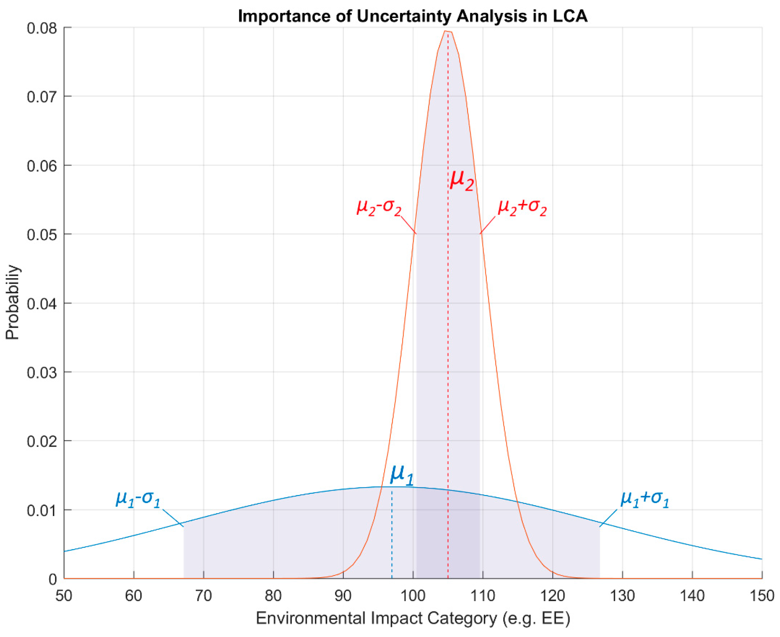
Figure 2.
Examples of three life cycle processes part of the primary data for this research.
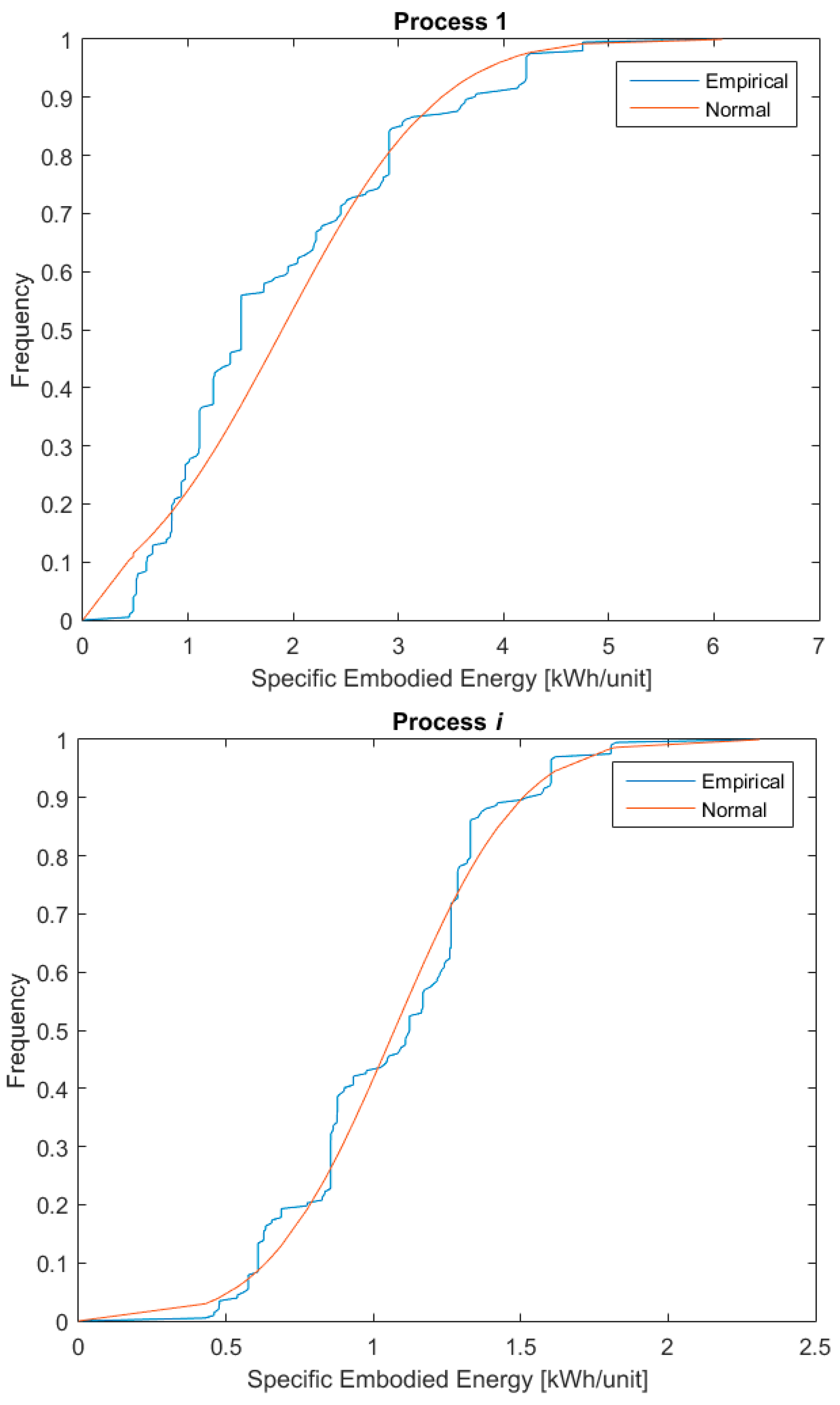
Figure 3.
Algorithmic approach developed for this research.

Figure 4.
Difference between results produced in MATLAB and Python for the mean values of embodied energy of the LCI.
Figure 4.
Difference between results produced in MATLAB and Python for the mean values of embodied energy of the LCI.
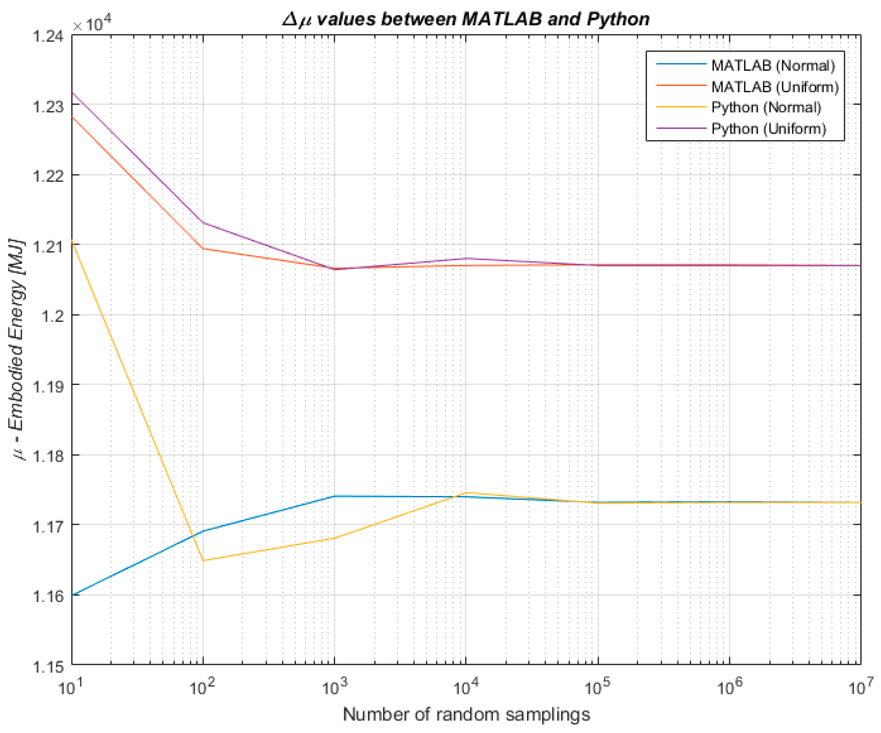
Figure 5.
Difference between results produced in MATLAB and Python for the standard deviation values of embodied energy of the life cycle inventory (LCI).
Figure 5.
Difference between results produced in MATLAB and Python for the standard deviation values of embodied energy of the life cycle inventory (LCI).

Figure 6.
Example of the results of the developed algorithm for one specific run (results refer to embodied energy (EE) (MJ) but are equal in trend in the case of embodied carbon (EC) (kgCO2e)).
Figure 6.
Example of the results of the developed algorithm for one specific run (results refer to embodied energy (EE) (MJ) but are equal in trend in the case of embodied carbon (EC) (kgCO2e)).
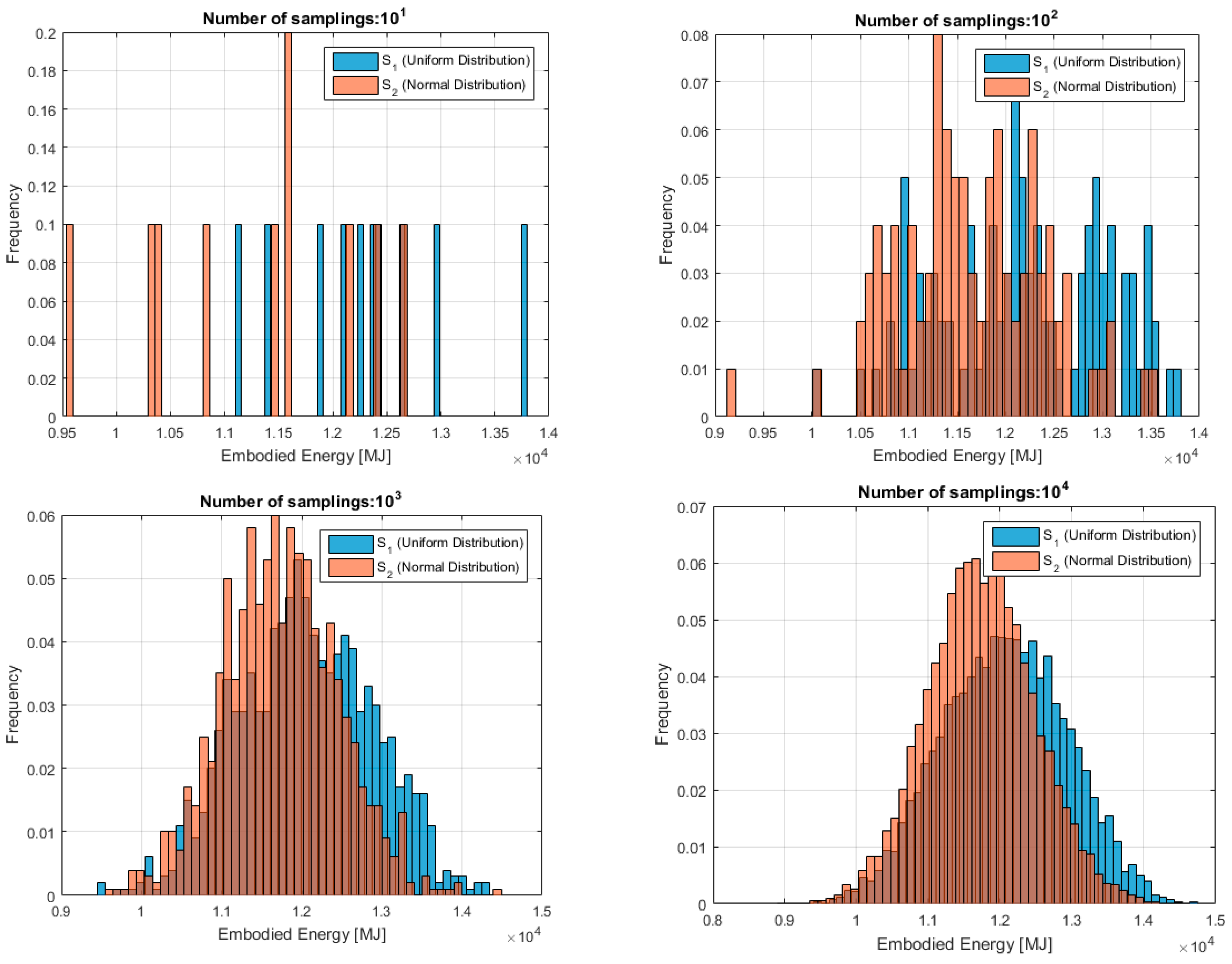
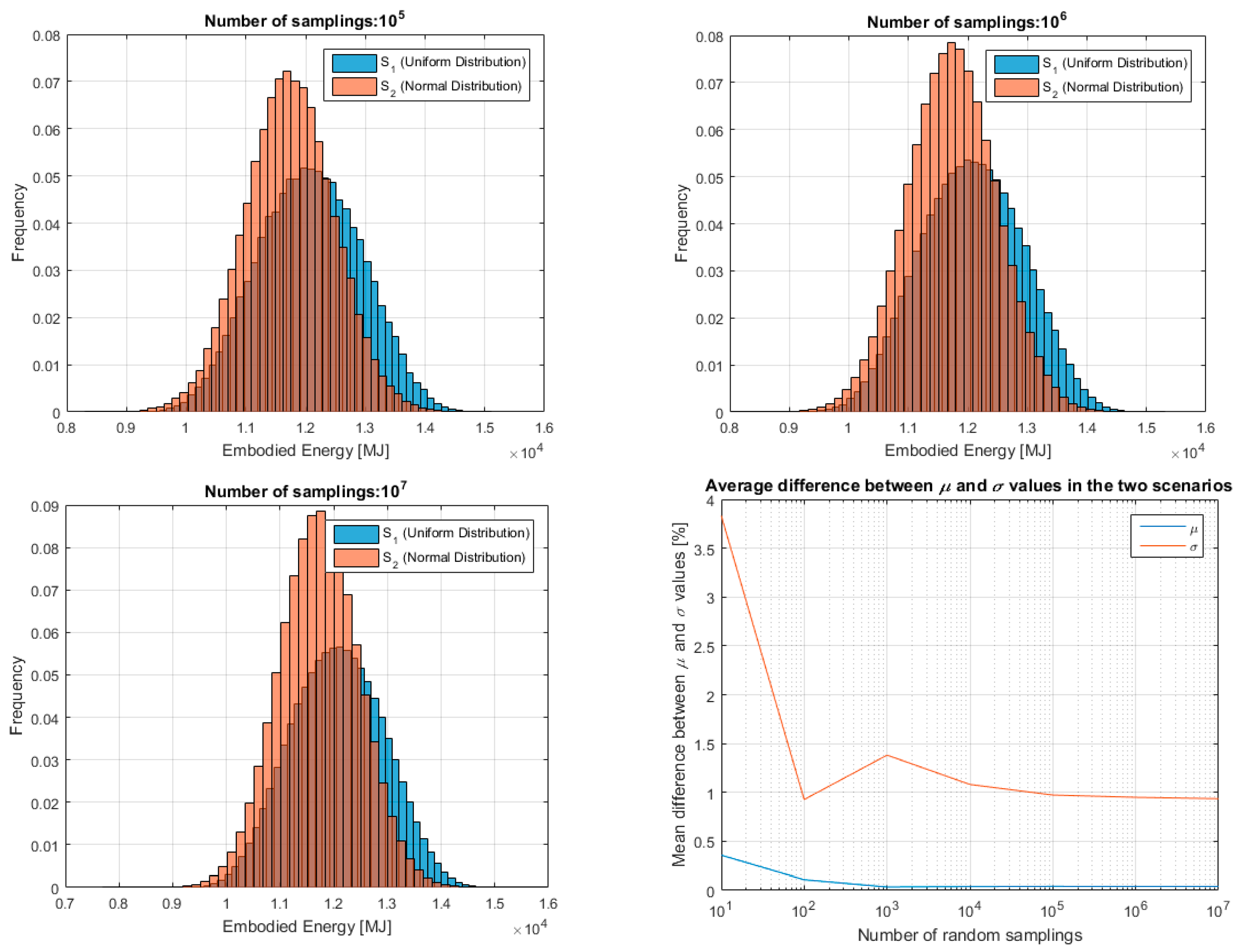
Figure 7.
μ and σ variation (percentage) between the two hypotheses across all 10 runs (only two LCI entries).
Figure 7.
μ and σ variation (percentage) between the two hypotheses across all 10 runs (only two LCI entries).
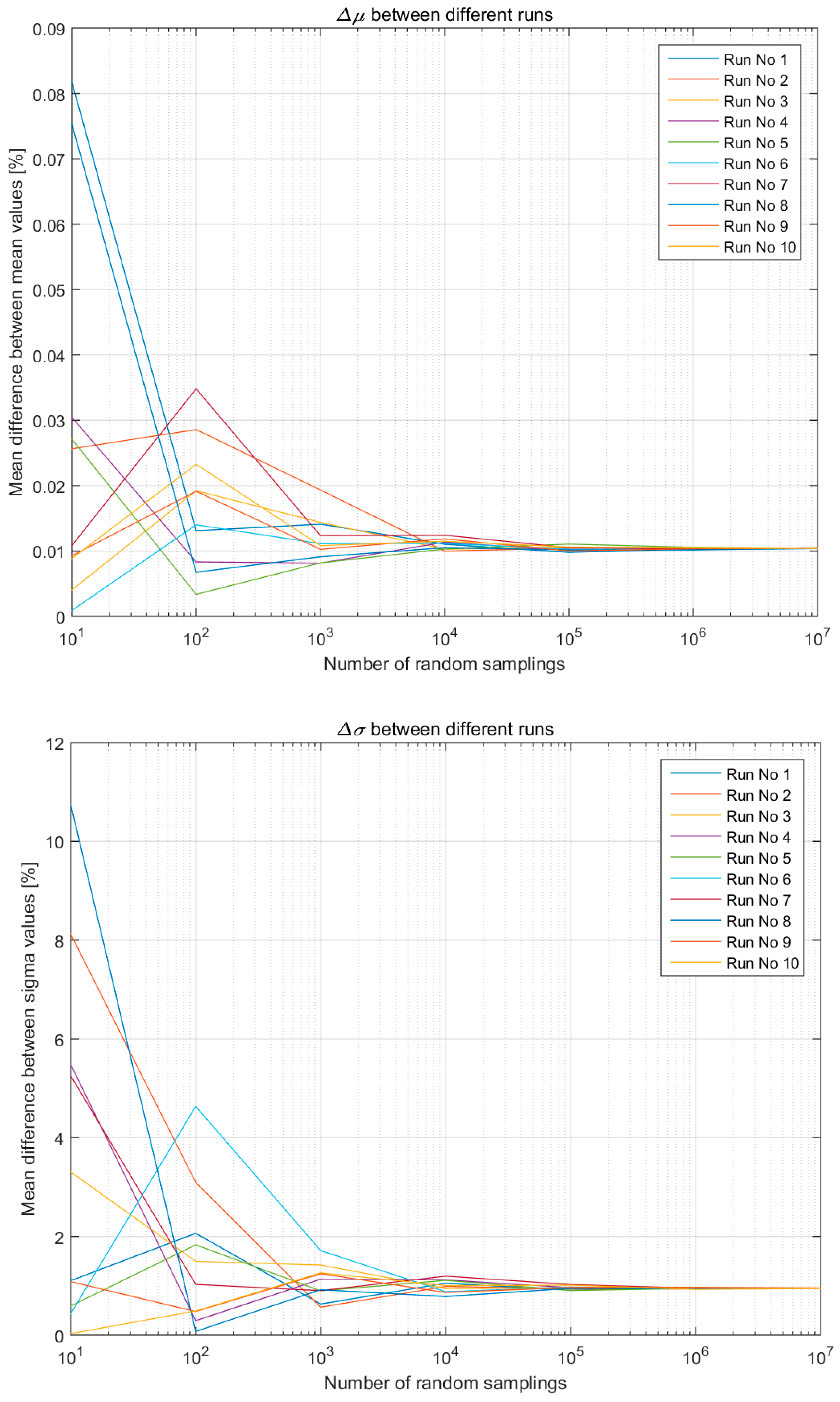
Figure 8.
μ and σ variation (percentage) between the two hypotheses across all 10 runs (for the full LCI).
Figure 8.
μ and σ variation (percentage) between the two hypotheses across all 10 runs (for the full LCI).

© 2017 by the authors. Licensee MDPI, Basel, Switzerland. This article is an open access article distributed under the terms and conditions of the Creative Commons Attribution (CC BY) license (http://creativecommons.org/licenses/by/4.0/).
Share and Cite
MDPI and ACS Style
Pomponi, F.; D’Amico, B.; Moncaster, A.M. A Method to Facilitate Uncertainty Analysis in LCAs of Buildings. Energies 2017, 10, 524. https://doi.org/10.3390/en10040524
AMA Style
Pomponi F, D’Amico B, Moncaster AM. A Method to Facilitate Uncertainty Analysis in LCAs of Buildings. Energies. 2017; 10(4):524. https://doi.org/10.3390/en10040524
Chicago/Turabian StylePomponi, Francesco, Bernardino D’Amico, and Alice M. Moncaster. 2017. "A Method to Facilitate Uncertainty Analysis in LCAs of Buildings" Energies 10, no. 4: 524. https://doi.org/10.3390/en10040524
Note that from the first issue of 2016, this journal uses article numbers instead of page numbers. See further details here.