1. Introduction
The power system is connected to generators, loads, and various power equipment through transmission lines, and is always exposed to disturbances, such as load fluctuations and line failures. In order to supply power stably during such disturbances, a controller, such as an excitation system or a governor, must operate properly. In large-scale power systems, wide area low frequency oscillation can threaten the stable operation of the system. Therefore, accurate estimation of the dominant oscillation mode is one of the important factors for stable operation of the system.
The oscillation in the power system occurs mainly in the low frequency range below 2.5 Hz, and in particular in the wide frequency mode, where it occurs below 1.0 Hz [
1,
2]. The local mode oscillates several generators, while the wide area mode simultaneously oscillates many generators. It is necessary to accurately estimate the local mode and the wide area mode for the stable operation of the system. So far, the analysis of low frequency oscillations in power systems has been performed mainly by eigenvalue analysis based on a linear model [
3,
4,
5,
6,
7]. However, eigenvalue analysis using a linear model does not accurately reflect the rapidly changing system environment, and modeling errors can occur [
8].
With the rapid development of digital technology and communication network technology since 1990, parameter estimation methods using measured data in power systems are actively being developed. Various algorithms have been proposed for estimating the oscillation mode in the acquired data. Among them, Prony analysis is the most frequently applied algorithm for the oscillation analysis of power systems [
9]. Trudnowski et al. [
10] proposed a method of estimating an oscillation mode using several signals, while Pierre et al. [
11] proposed a method of estimating the modal frequency and damping in ambient data using a Wiener-Hopf prediction equation.
Various research efforts have also proposed a method of system reduction by obtaining an equivalent model of the system using the residue and mode of the signal [
12,
13], a new method to design a PSS (power system stabilizer) controller, wide-area damping control [
14,
15,
16], and network equivalent modeling using Prony analysis [
17]. Grund et al. [
18] compared Prony analysis and eigenanalysis for generating frequency-domain data.
Sanchez-Gasca and Chow [
19] evaluated the performance of three identification methods; while other research has included an ARMA (auto-regressive moving average) block-processing technique to estimate the modes from measured ambient power system data [
20], a least squares and generalized least squares time-domain identification algorithm [
21], a regularized robust recursive least squares method [
22], time-frequency analysis method using resonance-based sparse signal decomposition and a frequency slice wavelet transform [
23], and an algorithm for the extended modified Yule Walker [
24]. Trudnowski [
25] and Shim et al. [
26] proposed a theoretical basis for estimating an electromechanical mode-shape; in addition, this is applied to various fields, such as fault location and accurate frequency estimation.
However, the parameter estimation methods applied to a power system are sensitive to sampling, time interval, and noise [
27]. Therefore, considerable experience and effort are required to estimate the accurate oscillation mode.
This paper proposes a multiple time interval (“multi-interval”) parameter estimation method that can simultaneously consider multiple time intervals. Linear prediction equations can be obtained from the measured signal. By solving the linear prediction equation, we can obtain the coefficients of the prediction error polynomial.
If multiple polynomials of the same order have the same root, the new polynomial summing the similar terms of each polynomial has the same root. Therefore, if the order of the prediction error polynomials obtained from several measurement data is the same, a new prediction error polynomial can be obtained by adding the coefficients of the respective polynomials.
Suppose that the signal acquired from the system contains an oscillation mode. If the signal is divided into several signals, the same oscillation mode is included in the separated signals. Therefore, a new prediction error equation can be formed by adding the coefficients of the respective prediction error equations that correspond to each time interval. Such a new prediction error equation is a multi-interval prediction error equation that considers multiple time intervals. Since the root of this equation is the oscillation mode included in the multiple time interval, it is possible to estimate the important mode by solving one equation for multiple time intervals or signals.
The parameter estimation method proposed in this paper is applied to the test function and the data acquired from the PMU (phasor measurement unit) installed in the KEPCO (Korea Electric Power Corporation) system. We confirmed the efficiency and reliability of the proposed algorithm.
This paper is organized as follows.
Section 2 describes the multi-interval parameter estimation.
Section 3 describes the September 2011 rolling blackout of the KEPCO system.
Section 4 describes the results of applying the algorithm proposed in this paper to the test function, while
Section 5 describes the results of applying it to the KEPCO system.
Section 6 summarizes the results, and
Section 7 concludes the paper.
2. Parameter Estimation Method of Multiple Time Intervals
2.1. Signal and Modal Decomposition
Assume that the measured signal consists of the sum of damped cosine functions. If the amplitude and phase of the
i-th cosine function are
Ai and
φi, respectively, and the damping coefficient and frequency are
αi and
ωi, respectively, the measured signal can be expressed as follows:
where,
N is the number of measured signals.
Using the damping coefficient and frequency, the complex mode can be expressed as
λi =
αi +
jωi. If the sampling is
T, the new complex mode
zi can be defined as follows:
If the Vandermonde matrix having the complex mode
zi as a matrix element is
V, the measured discrete signal can be decomposed as follows:
where the order of the Vandermonde matrix
V is
N ×
p, the order of the vector
B is
p × 1, and
p is the number of unknowns.
Therefore, the discrete signal sampled at an equal interval
T can be expressed as follows:
Since the discrete signal is represented by a set of impulses, if the sampling is too small, integer multiple modes for the critical mode can be estimated; while if the sampling is too large, aliasing with overlapping spectra can occur. Also, if the time interval is too large, the degree of the linear prediction matrix becomes large, which is not only burdensome to calculate, but can also produce inaccurate results. Therefore, when estimating parameters in a discrete signal, the selection of an appropriate sampling and time interval is very important.
2.2. Prediction Error Polynomial
The autoregressive moving average (ARMA) model of the discrete signal can be expressed as follows [
28]:
Assuming that the input signal
ut is an impulse signal, it can be expressed as follows:
From this equation, a linear prediction covariance equation with
ai as an unknown is obtained:
where if
p is the number of unknowns, the order of the matrix
Y is
N ×
p, and the order of
a is
p × 1.
From the linear minimum mean-squared error (LMMSE) estimation of the linear prediction, the prediction error polynomial with unknown coefficients can be expressed as follows:
The complex mode can be estimated by calculating the solution of the prediction error polynomial.
2.3. Prediction Error Polynomial of Multiple Time Intervals
In order to accurately estimate the important parameters in the measured signal, it is necessary to analyze and experience various sampling and time intervals. The result of the parameter estimation is greatly influenced by the number of unknowns (p), the sampling (T), the time interval (T0), and the number of data (N).
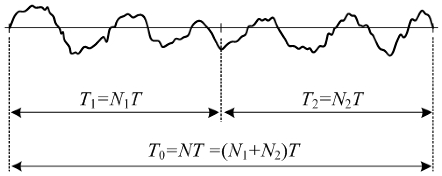
Since the time interval is the product of the sampling and the number of data, the entire time interval can be represented as
T0 =
NT.
Figure 1 shows that the other time intervals can be set differently, according to the number of data:
It is assumed that the same mode
z0 is included in the time intervals
T1 and
T2, as shown in
Figure 1. Then, the prediction error polynomial for the time interval
T1 can be expressed as follows [
28]:
where
p is an unknown number, and
A1(
z) is a prediction error polynomial corresponding to the time interval
T1.
The prediction error polynomial for the time interval
T2 can be expressed as follows:
Assume that several polynomials of the same order have one or more identical roots. Then a new polynomial, which is obtained by the summation of the similar term coefficients of each polynomial, has the same root.
Therefore, the new prediction error polynomials obtained from Equations (9) and (10) have the same mode
z0. The new prediction error polynomial obtained by the summation of the similar term coefficients of the two prediction error polynomials can be expressed as follows:
where,
a0 +
b0 = 2 and
ap +
bp = 0.
This equation is a prediction error polynomial for two time intervals in which the same mode exists. From this equation, it is possible to derive a generalized equation of the multi-interval prediction error polynomial, which can simultaneously consider multiple time intervals. If the same mode exists in the
n time intervals, the following equation is established:
In this equation, ci is the sum of the i-th coefficients of the prediction error polynomials for each time interval. If n = 1 in Equation (12), the prediction error polynomial for the entire time interval is obtained. Therefore, if the unknown number is fixed as p, it is possible to form a prediction error polynomial for various time intervals.
2.4. Procedure of the Multi-Interval Parameter Estimation
The procedure of the multi-interval parameter estimation algorithm proposed in this paper is as follows:
Step 1. Input the measured signal, and set the time interval (n) and the unknown number (p), as shown in Equation (12).
Step 2. For each selected time interval, form a covariance equation, as shown in Equation (7), and compute the unknown by solving the equation.
Step 3. Construct a new multi-interval prediction error polynomial, as shown in Equation (12), using the unknowns for each time interval.
Step 4. Calculate the complex mode, by finding the roots of the multi-interval prediction error polynomial.
Step 5. Construct the Vandermonde matrix with the complex mode, and find the residue corresponding to the mode using Equation (3).
Step 6. Restore the signal using the complex mode and the residue, and compute the SNR (signal-to-noise ratio) using the restoration signal and the original signal.
Step 7. Extract the dominant oscillation mode needed for the power system analysis from the estimated parameters.
3. Rolling Blackout of the KEPCO System
3.1. Situation of Rolling Blackouts and Implementation
When the load demand is larger than the power supply, interruptible load shedding is carried out to reduce the load. Such an artificial load interruption is the final resort that can be taken to ensure the stable operation of the power system; and if conducted properly, it is possible to prevent the collapse of the entire power system.
On 15 September 2011, a large-scale rolling blackout that cut off a total load of 5000 MW occurred in the KEPCO system. Forced load shedding was performed to prevent the collapse of the system due to the frequency drop. Since the power outage rate of the KEPCO system was relatively low, and the first nationwide power outage occurred, the rolling blackout caused great social confusion [
28].
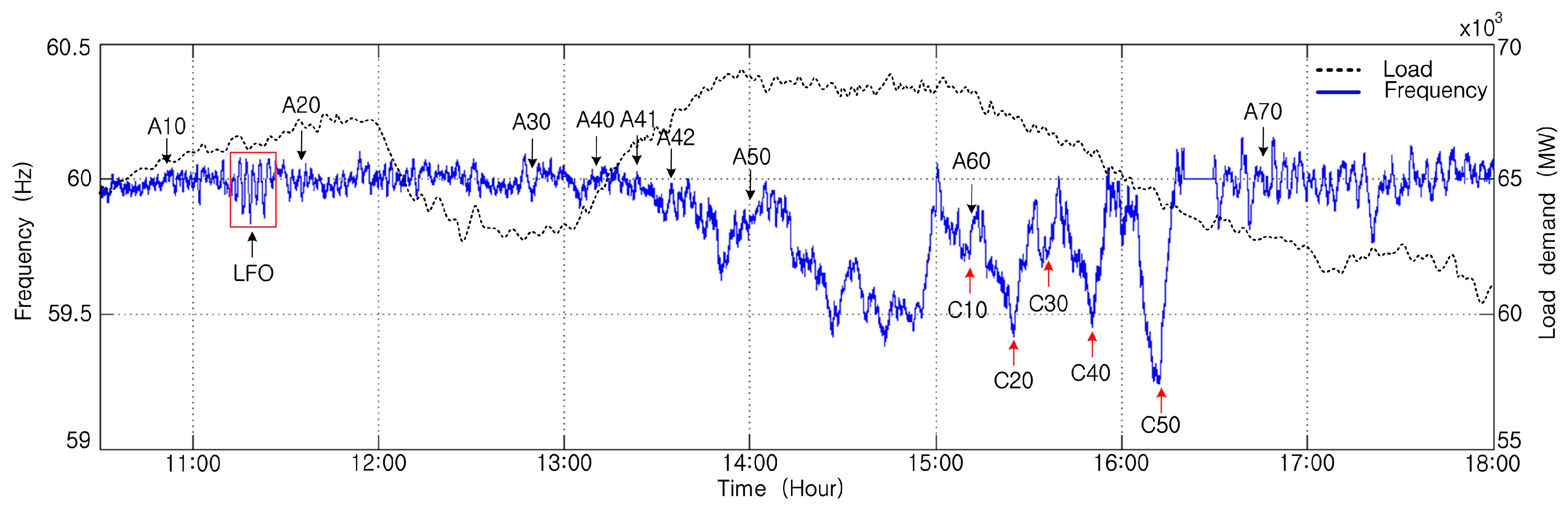
Figure 2 shows the total load and system frequency on the day of the rolling blackout. The situation of the power supply and load demand are very significant in a rolling blackout. The system with a supply capacity of 70.07 million kW and a maximum load of 64 million kW was operating normally by 11:00. Load demand increased steadily due to the sultry weather, and the amount of pumped-storage power generation that started from 08:00 continued to increase.
The reserve power decreased to below 4 million kW at 10:50 (A10), and decreased to less than 3 million kW at 11:35 (A20). After 13:00, the reserve power began to decrease again and decreased to 1 million kW or less at 13:35 (A42). The distribution transformer tab was adjusted at 12:50 (A30), and direct load control was enforced at 14:01 (A50). The first forced load shedding was implemented at 15:11 (C10), and the load was sequentially cut off by 1000 MW.
In
Figure 2, C10 to C50 represent the moments when the forced load shedding was implemented, and these show that after the forced load shedding, the system frequency recovered quickly.
The figure shows that the frequency of the system changed rapidly at about 11:20 (LFO). At that time, the reserve power was small, but there was no large disturbance, such as a line failure or generator trip. As a result, it can be seen that a small disturbance, such as a small variation of load or generation, can cause system oscillation.
3.2. PMU Data Measured in the KEPCO System
In this paper, the parameters were estimated by applying the multi-interval parameter estimation method to the data measured during the rolling blackout by the PMU installed at the East-Seoul substation. Recently, 40 PMUs have been installed in the KEPCO system. However, on the day of the rolling blackout in September 2011, only a few PMUs had been installed for testing purposes.
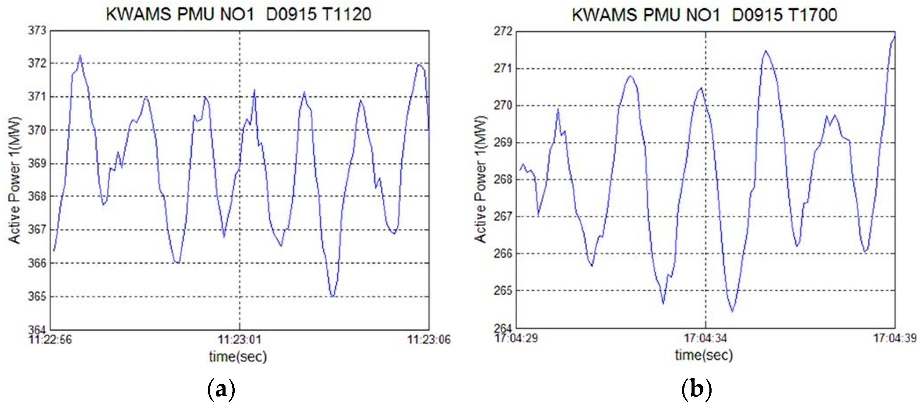
Figure 3 shows the active power at 11:00 and 17:00 on the data measured during the rolling blackout. The figure shows the periodically oscillating active power for 10 s. In the figure, “PMU NO1” refers to the PMU installed at the East-Seoul substation, while “D0915” and “T1120” refer to the date and time, respectively.
The active power shown in the figure is measured at the substation, and therefore represents the power flow. Unlike power plants, it is evident that the power flow of the substations is changing rapidly. A large variation of power flow is caused by load changes, power generation fluctuations, or the tripping of critical lines. Since no line failure occurred on the day of the rolling blackout, most of the power flow changes are likely due to the variation of the load or power generation.
Figure 3a shows that the variation of active power is about 6 MW, and changes about 1.6% based on 369 MW.
Figure 3b shows the variation of the active power to be about 7 MW, and that it fluctuates about 2.6% based on 268 MW. It can be seen that the fluctuation of the power flow is larger in the process of releasing the forced load shedding.
The power flow measured in steady state contains white noise. However the signals in
Figure 3 show relatively distinct periodic characteristics. These characteristics are caused by the inconsistency of the power flow between the regions. Therefore, it can be expected that the generators are oscillating with relatively larger amplitudes.
4. Examples for the Test Function
To test the multi-interval parameter estimation method described above, this paper defines the damped cosine function as Equation (13):
Table 1 shows that the test function consists of three damped sinusoidal functions, and shows the parameters of each function. Signals were generated by adding 5% and 30% noise to the cases shown in
Table 1, respectively. Then, the sampling was set to 1/10 s and 1/60 s, respectively, and parameters were estimated for the acquired signals for 10 s.
In order to compare the accuracy of the algorithm, this paper estimated the parameters 10 times for all cases. In the multi-interval parameter estimation method, the time interval
n = 2 and the unknown
p = 20 were set. Since random noise was added for every iteration, all of the results were slightly different.
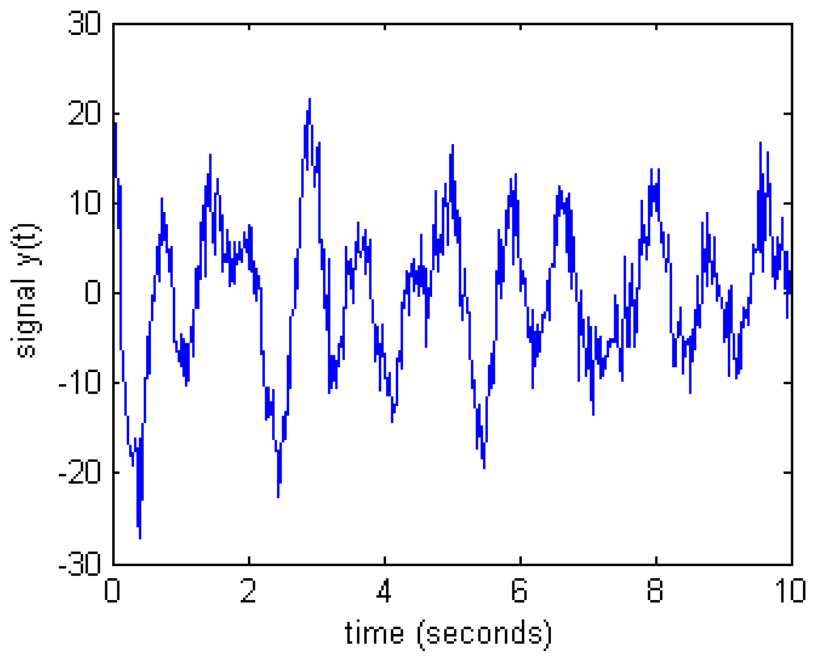
Figure 4 shows the signals with the sampling and damping coefficients set to 1/60 s and −0.01, respectively, with 30% noise added.
Table 2 shows the estimated modes for case 1 and case 2. The results shown in the table represent the average of the modes estimated from the 10 signals with random noise added. “ExPRO” in the table means the result obtained by applying the extended Prony method [
3,
14], while “MuPRO” means the result of the multi-interval parameter estimation method proposed in this paper. The “
dt” means sampling, “noise” is the added random noise, and “error” is the deviation of the exact mode and the estimated mode.
First, if the sampling was 1/10 s, both methods accurately estimated the modes within an acceptable tolerance. In the case of sampling 1/60 s and noise of 5%, ExPRO and MuPRO estimated the dominant modes included in the signal. However, the mode estimated by MuPRO was accurate, whereas the mode estimated by ExPRO had a large error. In the case of sampling 1/60 s and noise of 30%, ExPRO did not estimate the important mode included in the signal, but MuPRO estimated the important mode within an acceptable tolerance.
Table 3 shows the damping ratios and errors of the estimated modes. The damping ratio
ζi is computed from the real part (α
i) and the imaginary part (
ωi) of the mode shown in
Table 2, using the following equation:
The results shown in the table represent the average of the damping ratios estimated from the 10 signals. In the case of sampling 1/10 s, both methods accurately estimated the damping ratio within an acceptable tolerance. However, ExPRO estimated the damping ratio more accurately than MuPRO.
In the cases where the sampling and damping coefficients were 1/60 s and −0.01, and the noise was 5%, both methods estimated the damping ratio within an acceptable tolerance. However, when the sampling and damping coefficients were 1/60 s and −0.1, and the noise was 5%, MuPRO accurately estimated the damping ratio, whereas ExPRO did not.
In the case of sampling 1/60 s and noise of 30%, ExPRO did not estimate the damping ratio, but MuPRO estimated the damping ratio of the critical mode within an acceptable tolerance.
Table 4 shows the residue and error of the estimated mode. In the table, “ExPRO” and “MuPRO” mean the results obtained by applying the extended Prony method [
3] and the multi-interval parameter estimation method proposed in this paper. The results shown in the table are also the averages of the residues estimated from the 10 signals.
In the case of sampling 1/10 s, both methods accurately estimated the residue within an acceptable tolerance.
However, when the damping coefficient was −0.1 and the noise was 30%, the residues estimated in MuPRO and ExPRO were 11.706 and 13.721, respectively. When the noise was large, it can be seen that MuPRO estimated the residue more accurately.
When the sampling and the noise were at 1/60 s and 5%, respectively, the ExPRO estimated the residue with a large error, but MuPRO estimated the residue within an acceptable tolerance. In the case of sampling 1/60 s and noise of 30%, the residue was not estimated in ExPRO, while the residue in MuPRO was estimated within the tolerance range.
Table 5 shows the result of the phase estimation. When the sampling was 1/10 s, both methods accurately estimated the phase within the tolerance range regardless of the noise and damping coefficient, as in the previous cases. However, when the sampling was 1/60 s and the noise was 5%, the phase estimated by ExPRO had a large error, whereas the estimated phase in MuPRO was accurate within an acceptable tolerance. In the case of sampling 1/60 s and noise of 30%, ExPRO could not estimate the phase. On the other hand, MuPRO estimated the phase approximately.
Table 6 shows the signal-to-noise ratio (
SNR). The
SNR shown in the table is computed by the following Equation (15) [
9]:
where,
and
are the estimated signals and measured signals, and
is the mean square root. The larger the
SNR, the more accurately the signal is estimated.
Table 6 shows that ExPRO had a larger
SNR at sampling 1/10 s, but there was no significant difference. However, at sampling 1/60 s, the
SNR in MuPRO was much larger. In particular, when the noise was 30%, the
SNR in ExPRO was very small, and it was hard to estimate the parameter. On the other hand, it can be seen that the
SNR in MuPRO had a relatively large value, so that the parameters were estimated more accurately.
4.1. Mode and Residue Comparison
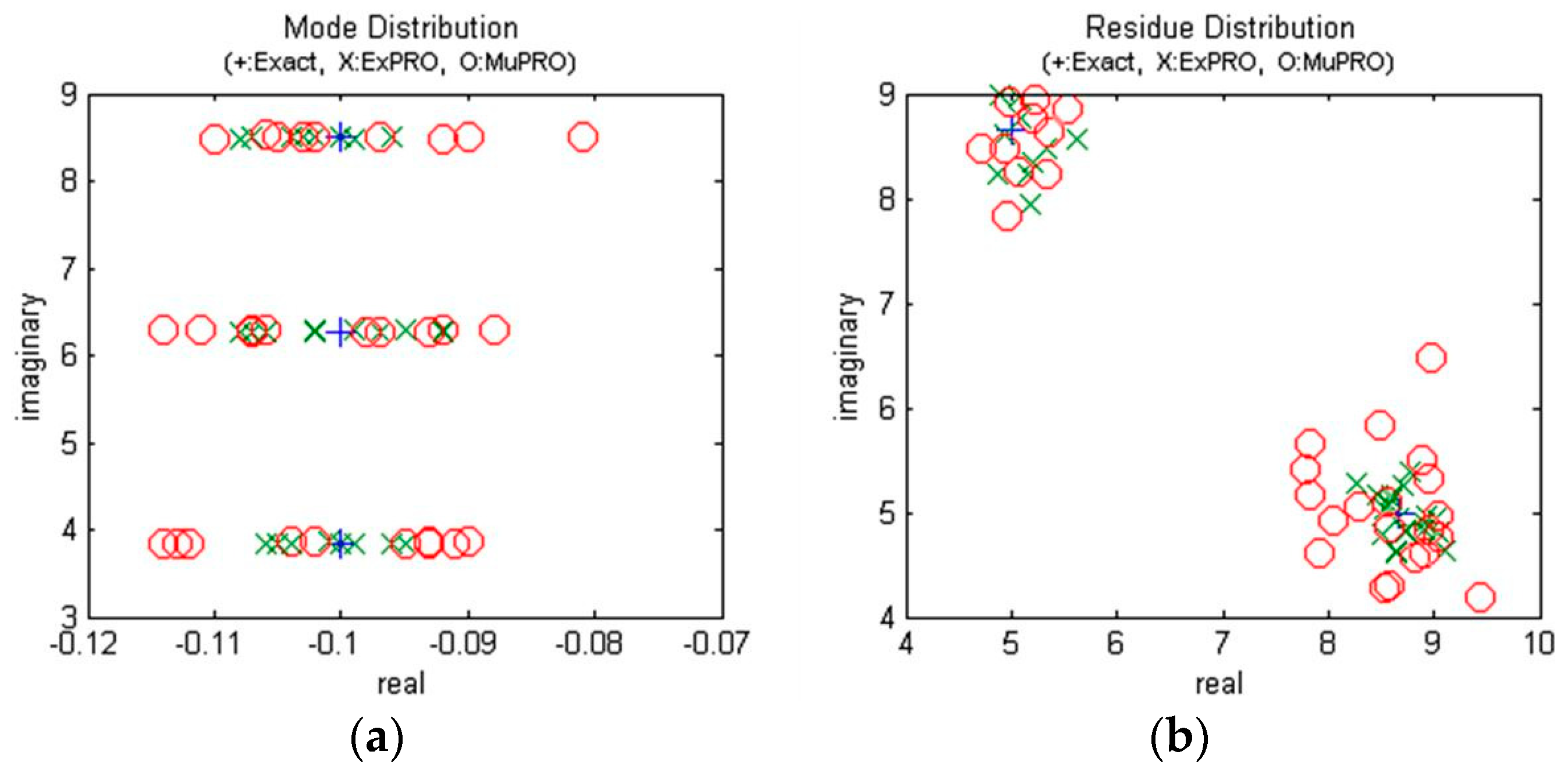
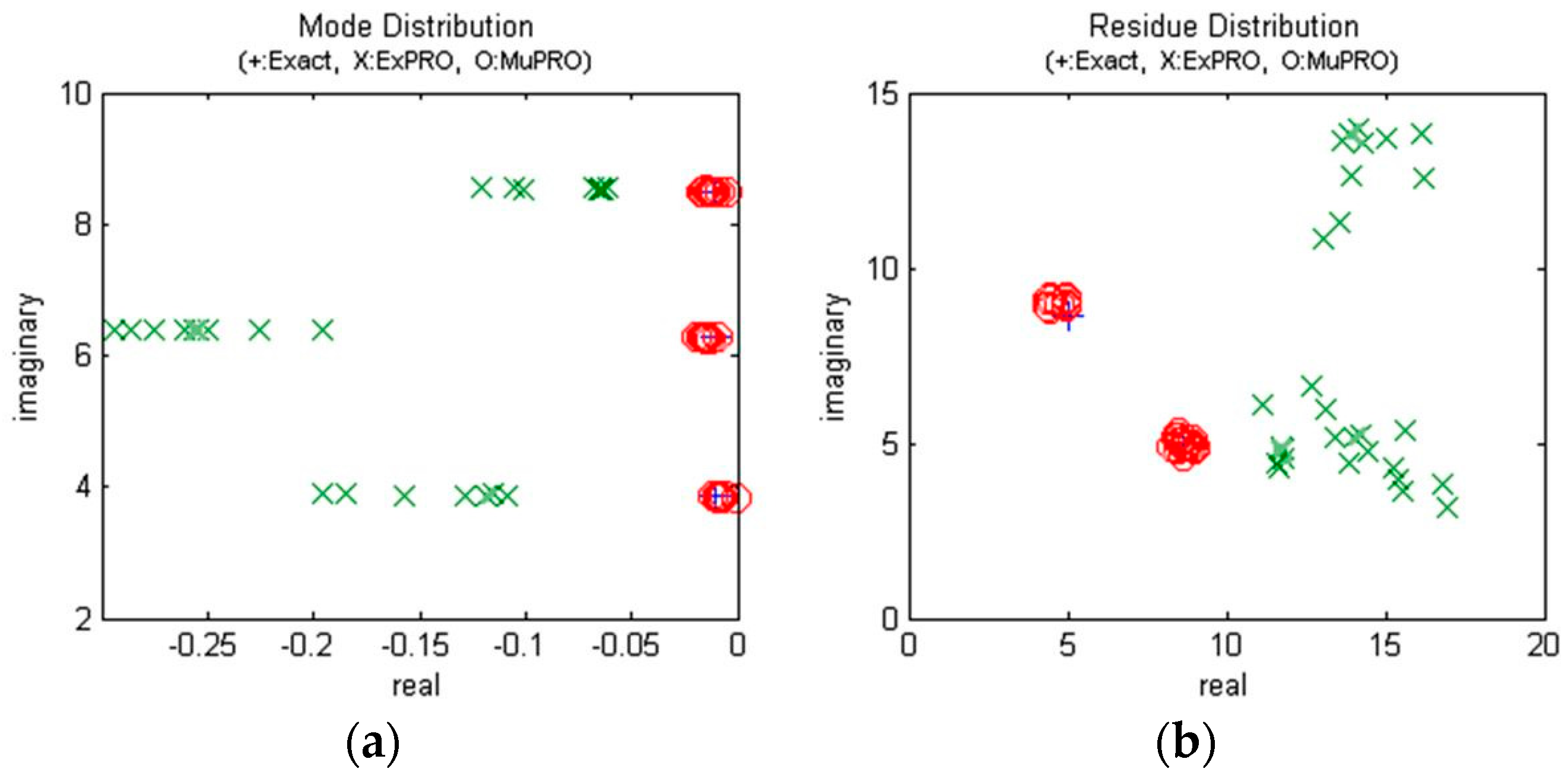
Figure 5 and
Figure 6 represent the estimated mode and residue for 10 signals with 5% random noise added. In the figure, “*” indicates the correct mode, and “O” and “X” indicate the parameters estimated by MuPRO and ExPRO, respectively.
Figure 5 shows the mode and the residue for sampling 1/10 s and damping coefficient −0.1. Both methods estimated the exact parameters, but ExPRO estimated the modes more accurately than MuPRO. However, all the estimated results were within the tolerance range.
Figure 6 shows the mode and the residue for sampling 1/60 s and damping coefficient −0.01. The figure shows that MuPRO estimated the mode and residue more accurately than ExPRO.
4.2. Estimation Signal Comparison
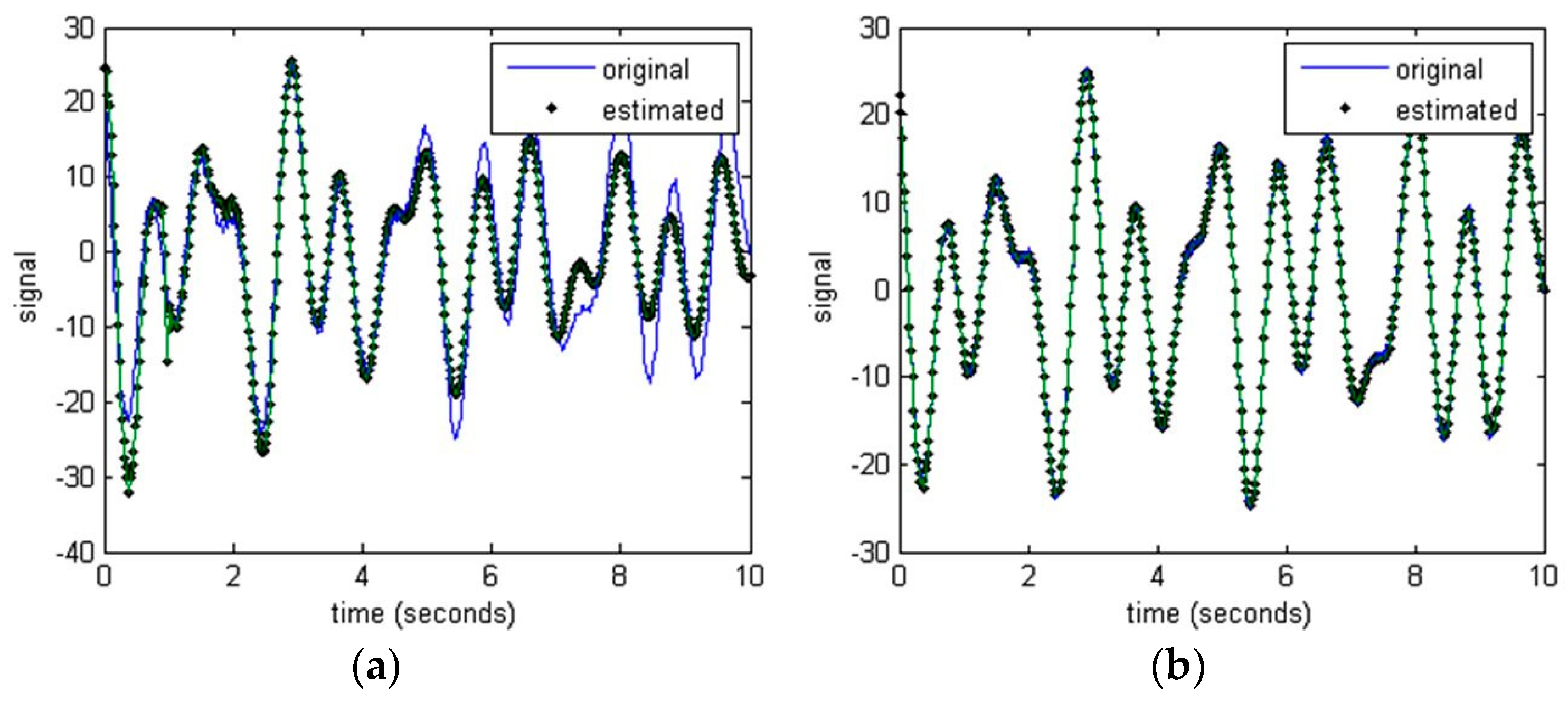
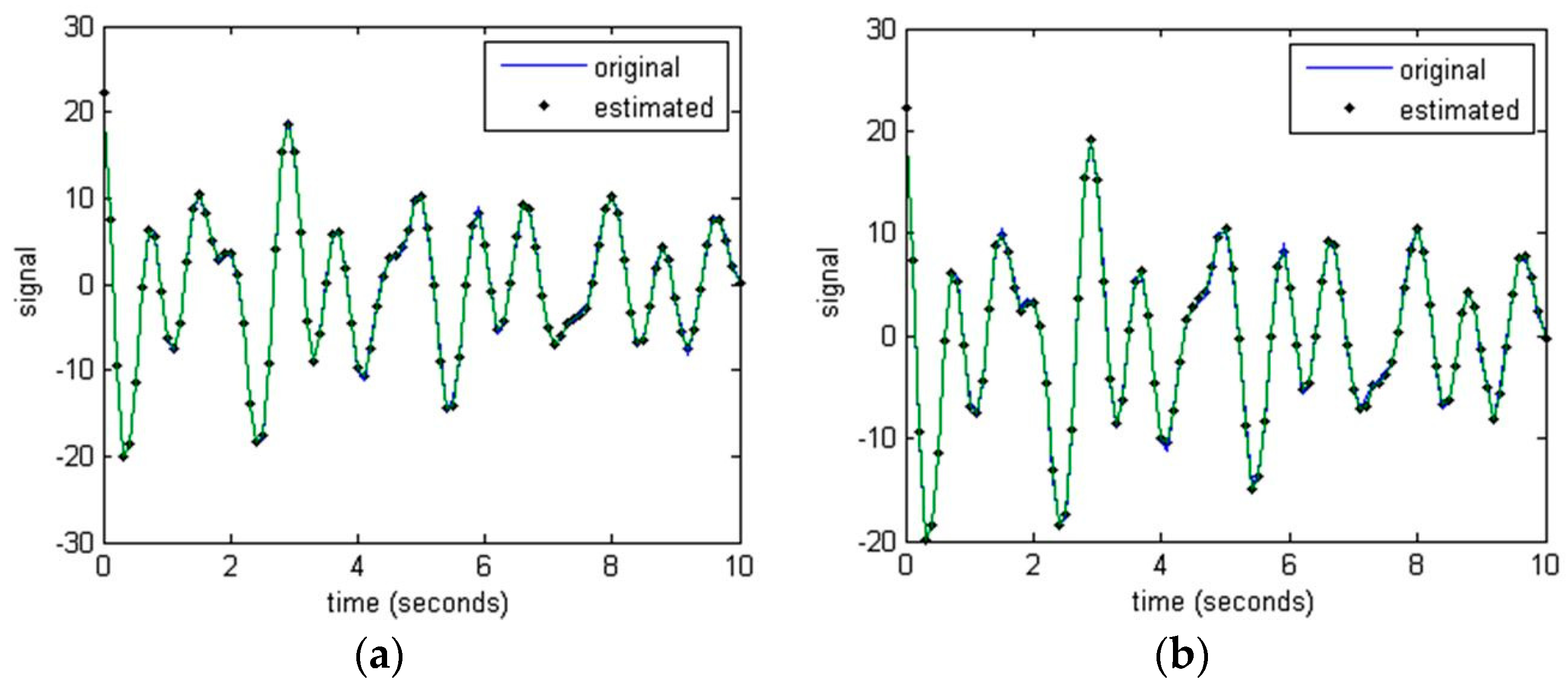
Figure 7 and
Figure 8 represent the comparison between the estimated signal and the original signal.
Figure 7a,b show the signals estimated by ExPRO and MuPRO when the sampling was 1/10 s and the damping coefficient was −0.01, respectively, and the original signal. In this case, the sampling was relatively properly chosen, and both methods accurately estimated the signal.
Figure 8a,b show the signals estimated by ExPRO and MuPRO when the sampling was 1/60 s and the damping coefficient was −0.01, respectively, and the original signal. It can be seen that the signal estimated by MuPRO was much more accurate than the signal estimated by ExPRO. The signal estimated by MuPRO was estimated similarly for the whole time interval. However, the signal estimated by ExPRO was initially approximated, but it can be seen that an error occurred over time.
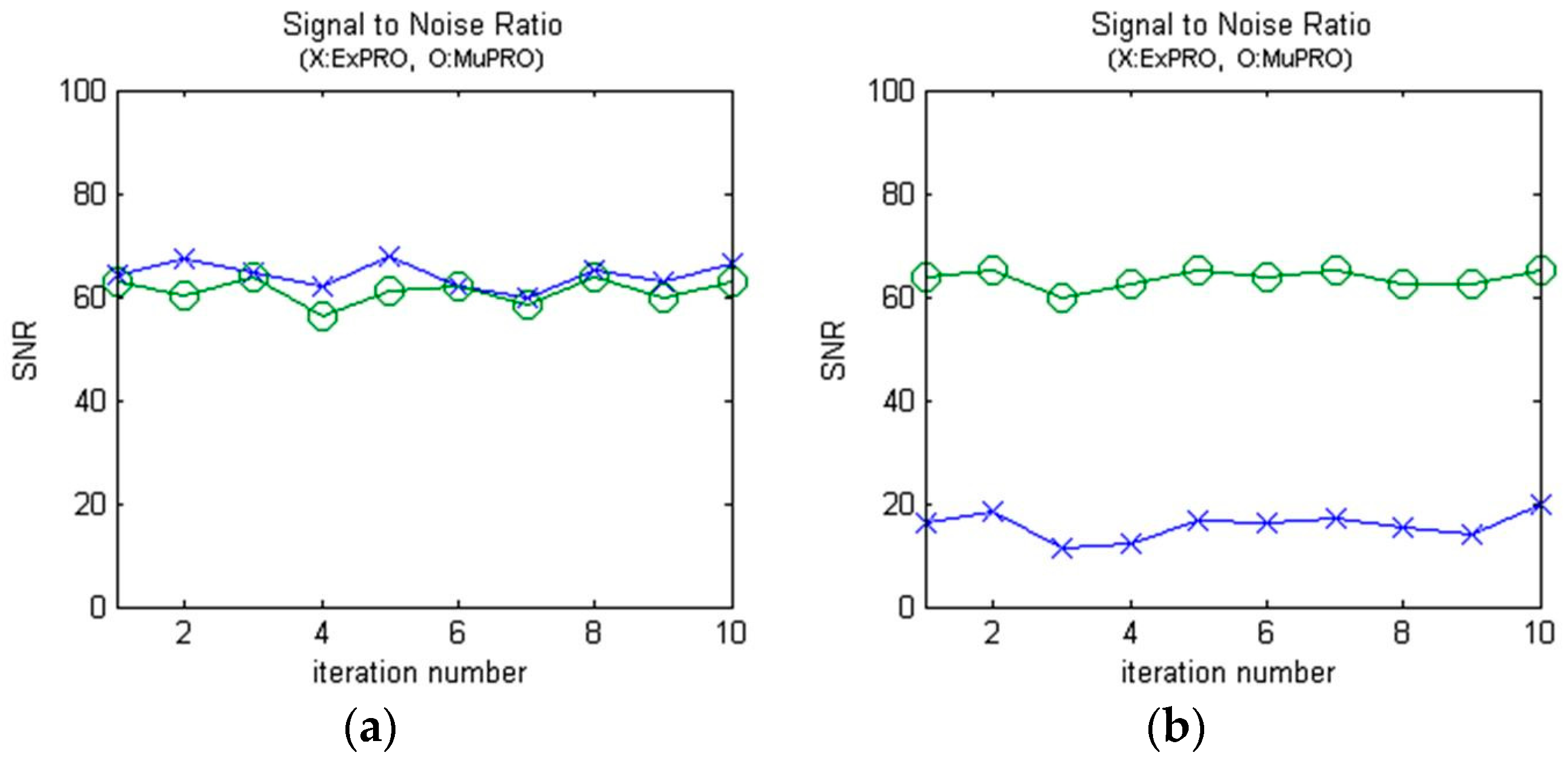
4.3. Signal-to-Noise Ratio Comparison
Figure 9 shows the
SNR computed by Equation (15). Each figure is the
SNR computed for the signal with 5% random noise added.
Figure 9a shows the
SNR computed when the sampling was 1/10 s and the damping coefficient was −0.1. In the figure, “X” and “O” represent the
SNR estimated by ExPRO and MuPRO, respectively.
Figure 9a shows that the
SNR of the signal estimated by ExPRO was larger than the
SNR estimated by MuPRO. However, both methods had a large
SNR, and thus accurately estimated the signal.
Figure 9b shows the
SNR estimated by ExPRO and MuPRO when the sampling was 1/60 s and the damping coefficient was −0.01. The figure shows that the
SNR estimated by MuPRO was much larger than the
SNR estimated by ExPRO. This shows that MuPRO estimated the parameters more accurately when the sampling was 1/60 s.
5. Results of the KEPCO System
The rolling blackout implemented in the KEPCO system in September 2011 was a relatively long-lasting failure. The actual rolling blackout started at 15:11 with forced load shedding, and ended at 19:56 [
29].
However, in terms of system operation, it is necessary to analyze the system from the time when the frequency fluctuation starts to occur due to the reserve power shortage, rather than the load shedding. At 10:50, the reserve power decreased to less than 4 million kW. Considered from this time, the rolling blackout can be treated as a system failure that lasted for 9 h.
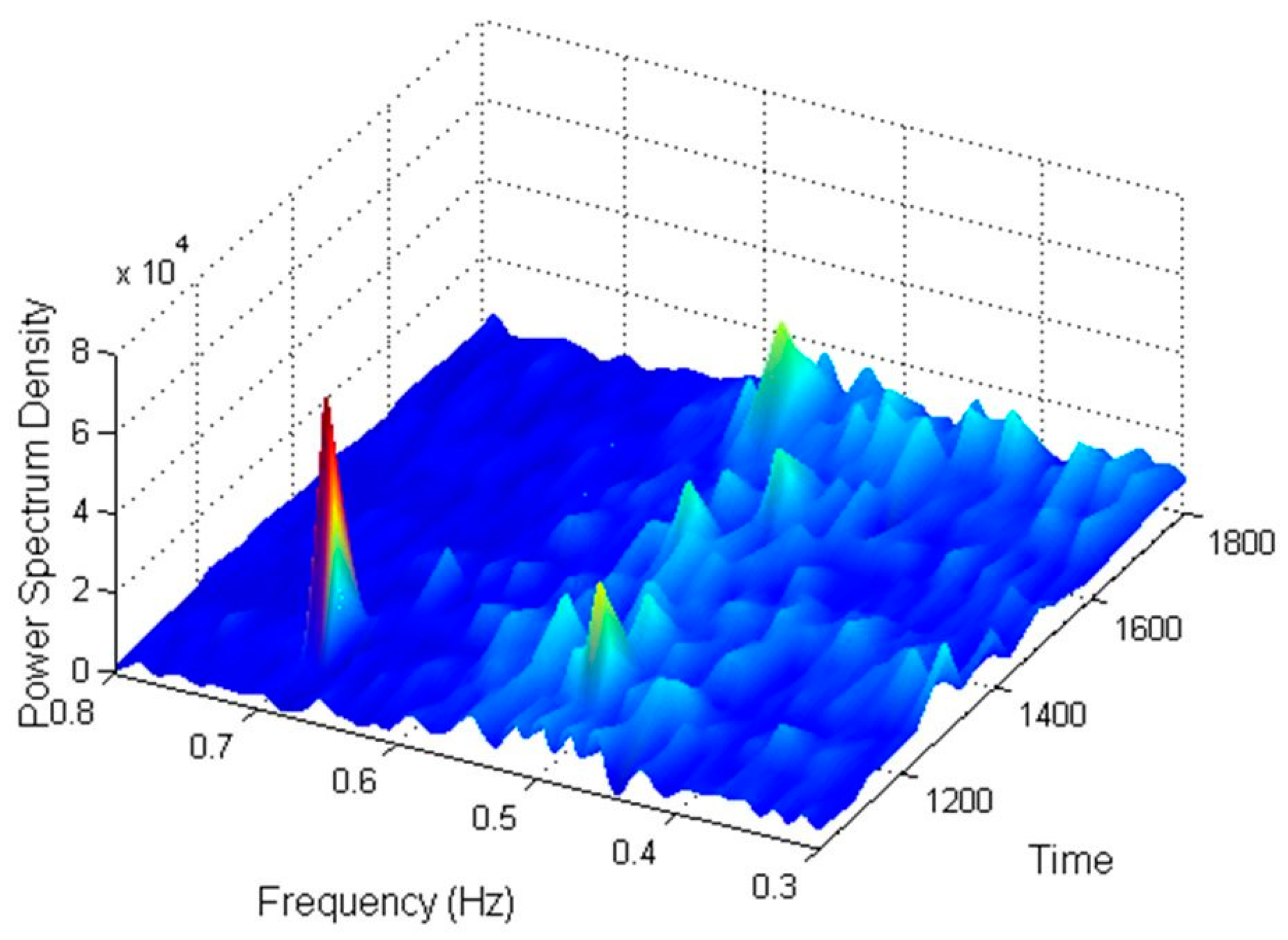
In this paper, spectral analysis and mode analysis are applied to the PMU data measured at the East Seoul substation on the day of the rolling blackout. Since the PMU data was measured at the substation, the cross spectral density (CSD) is meaningless. Therefore, only the power spectral density (PSD) is applied to analyze the rolling blackout.
Figure 10 shows the PSD computed from the power flow measured on the day of the rolling blackout. The figure represents the power spectrum magnitude and frequency from 10:30 to 18:00 during the rolling blackout. In the figure, the power spectral density of 0.68 Hz was very large. The oscillation of the frequency 0.68 Hz continued from 11:20 to 11:45. At this time, the power flow fluctuated greatly.
The frequency 0.68 Hz is a typical wide area mode frequency, but it is difficult to determine the exact cause of the oscillation, because no data was measured in the power plant. However, at this time there was an attempt to insert a small generator into the grid. Therefore, there is a high possibility that the system was fluctuating due to an inappropriate generator insertion in the absence of generation capacity. These oscillations are critical to system operation, because such a wide area oscillation can cause a blackout, and there is no clear countermeasure against it. If forced load shedding is applied according to the system frequency drop such as a rolling blackout, the load shedding should be executed, so that the wide area mode is not activated. After 17:00, the power spectrum density near the frequency 0.55 Hz was large during the process of load restoration. Therefore, it can be seen that the load restoration should be performed properly.
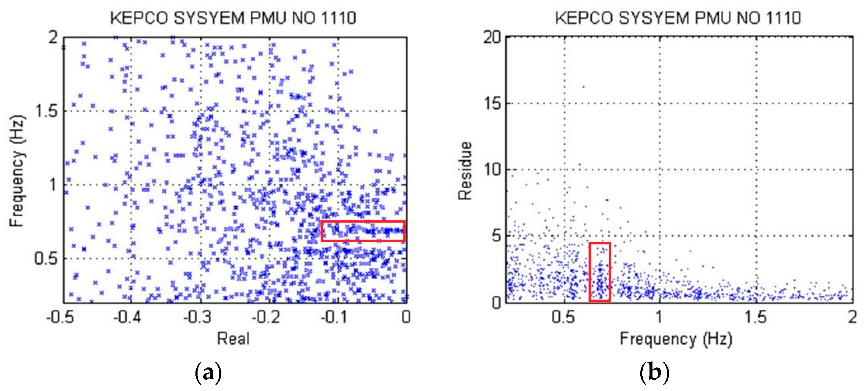
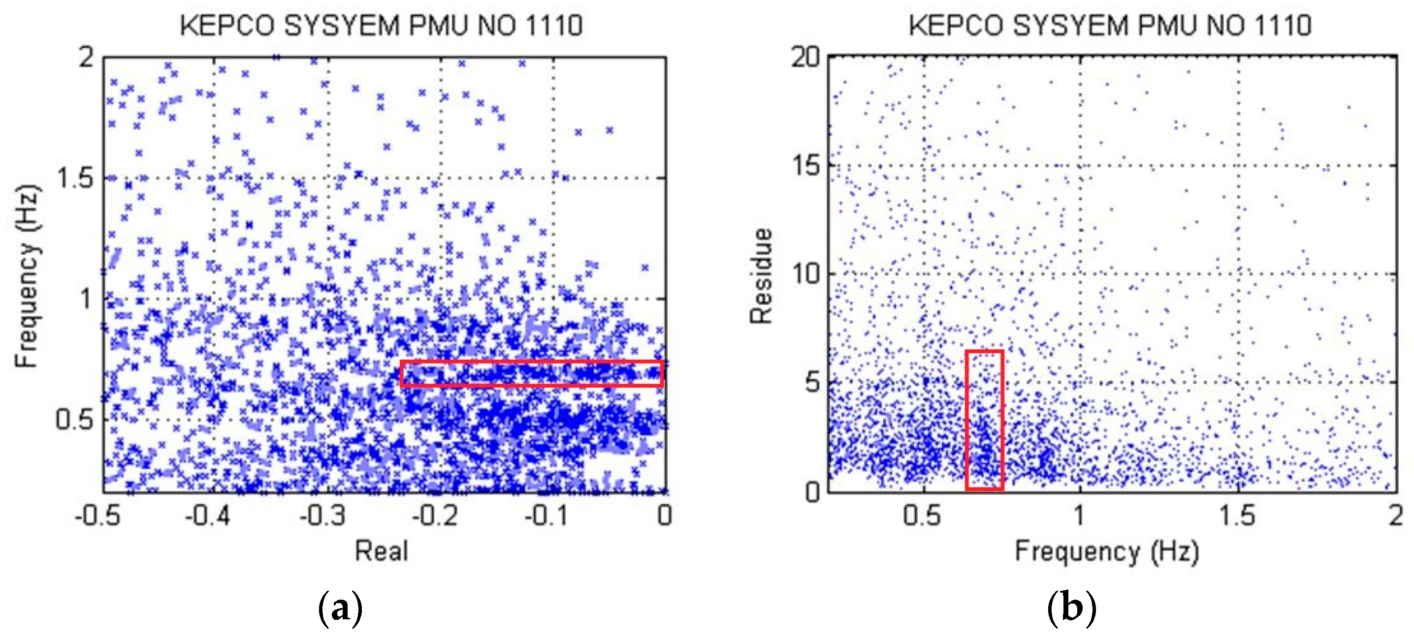
Figure 11 and
Figure 12 represent the parameters estimated by applying the extended Prony method (ExPRO) and the multi-interval parameter estimation method (MuPRO) for the power flow measured by the PMU on the day of the rolling blackout. The time interval and the shifting time were set to 10 s and 1 s, respectively. The sampling rate was set to 1/10 s, and the parameters were continuously estimated for the 40 minute data. In the multi-interval parameter estimation method, the time interval were set to 5 s (
n = 2). The modes and residues shown in the figure are expressed only when the
SNR was more than 10 dB.
Figure 11a shows the mode estimated by ExPRO, where the real part of the mode is the
x-axis, and the imaginary part is the
y-axis.
Figure 11b shows the residue magnitude with respect to the frequency. In both the mode and the residue, the dots are concentrated around the frequency 0.68 Hz.
Figure 12a,b show the mode and residue magnitude estimated by MuPRO proposed in this paper. In this case, the dots are also concentrated near the frequency 0.68 Hz.
These results are similar to the results of the power spectrum shown in
Figure 10. Therefore, it can be seen that the dominant mode of low frequency oscillation that occurred at 11:20 on the day of the rolling blackout was 0.68 Hz.
Figure 11 and
Figure 12 show that MuPRO estimated many more modes than ExPRO. Each figure shows the modes where the
SNR was more than 10 dB. Therefore, MuPRO estimated the mode more accurately than ExPRO.
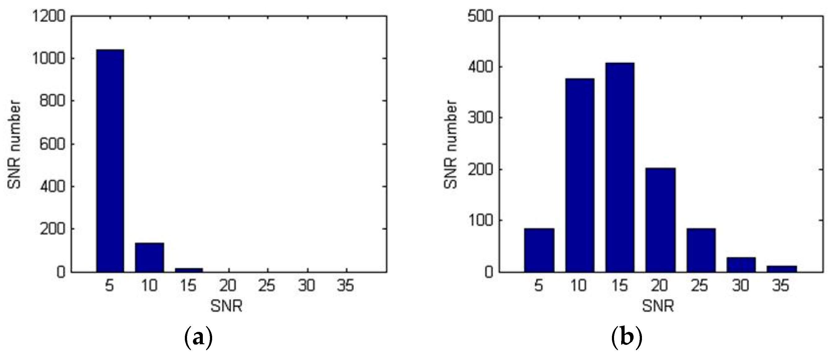
Table 7 shows the number of
SNRs computed from the estimated parameters. For the time interval
T = 10 s, the
SNR of 1,195 was computed. When
T = 20 s, the
SNR of 1,190 was computed.
The table shows that more than 70% of the
SNR computed by ExPRO was less than 5 dB. However, in MuPRO, more than 50% of the
SNR was larger than 10 dB. This shows that the MuPRO estimated the parameters more accurately than ExPRO, even for the data acquired in the real system.
Figure 13 represents the results shown in
Table 7, which shows that MuPRO estimated the parameters much more accurately than ExPRO.
6. Summary and Discussion
This paper describes the multi-interval parameter estimation method and its application results. The proposed algorithm was applied to the test function and the data was measured by the PMU installed in the KEPCO system. The parameters were estimated for changes in sampling, noise, and damping coefficients. Random noise was added to the given condition, the parameters were estimated 10 times, and the results were compared.
Neither the MuPRO nor ExPRO were sensitive to changes in the damping coefficient. Both methods also estimated the parameters within an acceptable tolerance for noise. However, when the sampling was 1/60 s and the noise was small, MuPRO accurately estimated the parameter, but ExPRO inaccurately estimated it. When the sampling was 1/60 s and the noise was large, ExPRO did not estimate the dominant parameter, but MuPRO accurately estimated the parameter. It can be seen that the proposed multi-interval parameter estimation method robustly estimates the parameters for noise and sampling.
The proposed method was applied to the data acquired during a rolling blackout of the KEPCO system. We repeatedly estimated the parameters by shifting the time interval. As a result, the SNR of MuPRO was larger than the SNR of ExPRO. MuPRO more accurately estimates the parameters for the data acquired from the actual system.
The signal measured in the power system includes random noise. The power system has inherent low frequency oscillation. Additionally, since the oscillation mode of the system cannot be accurately known, it is difficult to select the optimum sampling. Therefore, the multi-interval parameter estimation method is robust to noise and sampling, and thus it is more reliable in estimating the dominant oscillation modes in the power system.
7. Conclusions
This paper describes a multi-interval parameter estimation method that simultaneously considers multiple time intervals. When multiple polynomials of the same order have the same root, this same root is included in the new polynomial obtained by summation of the similar term coefficients of the polynomials. Therefore, if the same mode exists in multiple time intervals, a new multi-interval prediction error polynomial can be formed by adding the coefficients of the prediction error polynomials that correspond to each time interval.
The root of the multi-interval prediction error polynomial includes the important mode included in each time interval. Therefore, it is possible to estimate the dominant parameters included in multiple time intervals with one unknown calculation.
The multi-interval parameter estimation method is a very efficient algorithm in terms of accuracy and reliability, and is an algorithm suitable for low frequency oscillation analysis of the power system. The algorithm of the proposed multi-interval parameter estimation method was applied to the test function and to the data acquired from the PMU installed in the KEPCO system. As a result, it is confirmed that the multi-interval parameter estimation method accurately and reliably estimates important parameters.


