
Energy Demand Modeling Methodology of Key State Transitions of Turning Processes

1
Department of Industrial Engineering, Shandong University of Science and Technology, Qingdao 266590, China
2
Key Laboratory of Contemporary Design and Integrated Manufacturing Technology, Ministry of Education, Northwestern Polytechnical University, Xi’an 710072, China
*
Authors to whom correspondence should be addressed.
Energies 2017, 10(4), 462; https://doi.org/10.3390/en10040462
Submission received: 5 January 2017
/
Revised: 5 March 2017
/
Accepted: 24 March 2017
/
Published: 2 April 2017
(This article belongs to the Special Issue Energy Efficient Manufacturing)
Abstract
:Energy demand modeling of machining processes is the foundation of energy optimization. Energy demand of machining state transition is integral to the energy requirements of the machining process. However, research focus on energy modeling of state transition is scarce. To fill this gap, an energy demand modeling methodology of key state transitions of the turning process is proposed. The establishment of an energy demand model of state transition could improve the accuracy of the energy model of the machining process, which also provides an accurate model and reliable data for energy optimization of the machining process. Finally, case studies were conducted on a CK6153i CNC lathe, the results demonstrating that predictive accuracy with the proposed method is generally above 90% for the state transition cases.
1. Introduction
The report of the International Energy Agency (IEA) revealed that nearly one-third of global energy use and 40% of carbon dioxide (CO2) emissions are attributable to the manufacturing industry [1]. It is evident that the manufacturing industry has become one of the major sources of energy consumption and CO2 emissions, which will continue to increase by 1.9% annually if no effective action is taken [2]. Improved industrial energy efficiency is a critical cornerstone in climate change mitigation [3]. Therefore, the manufacturing industry must take responsibility and strive to adopt more energy-efficient and sustainable production techniques [4]. If energy data and information can be more effectively used and analyzed in manufacturing, it will provide considerable insights into energy-saving opportunities [5]. The machining process, as one of the major processes of manufacturing industries [6], is vital to energy saving and emission reduction. Generally, the life cycle of a product can be divided into several stages: material production; manufacture and assembly; transport; use; and end-of-life. Machine tools follow the same pattern and its Life Cycle Analysis (LCA) has shown that 95% of the environmental impact of a machine tool is associated with its use phase (assuming a 10-year lifespan). Of that use phase impact, 95% comes from energy consumption [7]. However, because the life cycle of a machine tool is usually more than 15 years, even reaching up to 20 years (with the current trends indicating that the industry will most likely want to prolong their lifecycle) [8,9], the environmental impact from the use phase of machine tools tends to be greater than 95%, even going as high to 99%. Similar results in another study [10] have shown that CO2 emissions caused by the energy consumption of a computer numerical control (CNC) machine tool (spindle power is 22 kW) over one year was equivalent to the CO2 emissions of 61 SUVs.
It thus becomes clear that the energy consumption and emissions derived from the machining process is very significant. Triggered by the necessity to improve the energy efficiency and environmental performance of the manufacturing industry, energy modeling [11,12,13,14,15,16], energy-efficiency improvement [17,18,19,20,21,22] and carbon-emission reduction [23,24] of the manufacturing industry have been studied. Experiments show that power peaks will be caused by state transitions during the machining process [25,26], as shown in Figure 1. State transition indicates the transition process between the two neighboring states during the machining process, such as spindle startup, rapid positioning acceleration, coolant startup, tool change startup, etc. State transition generally relates to the instantaneous startup of the motor, as well as the instant momentum through increase of torque or moving parts, etc., which result in power increase and the subsequent phenomenon of peak power. However, intensive research about energy consumption characteristics and models of state transitions is scarce. To fill this gap, an energy demand modeling method for state transition of the turning process is proposed in this paper.
The peak power caused by machining state transition has been mentioned in many references [25,26,27]. However, the mechanism and energy demand model of the power peak has not been researched in depth; the existing studies have only demonstrated the phenomenon of peak power in the power curve. The duration of state transition is short, but the peak power caused by the state transition is high [27,28], making the energy demand of the state transitions significant. Moreover, state transitions occur frequently during the machining processes. The energy demand of state transition was not considered in reference [29]; therefore, the predicted energy is 9.3% less than the measured energy in the machining case. It can be observed that the energy demand of state transition is a vital part of the energy demand of the entire machining process.
Although the power peak of the spindle startup was measured in the literature [30], its energy demand was not. The spindle and feed axis acceleration power models were studied based on the torque and angular velocity [31]; however, the friction torque and the torque for overcoming the spindle rotational inertia involved in the models are very difficult to obtain, making the established models difficult to apply in real machining cases. Shi et al. measured the energy consumption of spindle from stopping state to different speeds and obtained the spindle startup energy model through quadratic function fitting [32]; the established model can be used to calculate the spindle startup energy from stopping to the specified speed. When the initial spindle speed is not zero (accelerating from low speed to high speed), the above model will not be applicable. Moreover, as shown in the energy supply model of the spindle startup established in our previous work [33], the model can only calculate the energy consumption of the spindle system during spindle speedup. However, during the spindle speedup process, standby operation, X,Y,Z-axis feeding, chip conveying, cutting flood spraying and other motions can also be executed. The actual energy demand of the spindle speedup is the sum of the energy demand of all the listed motions. Whether those motions are executed or not during spindle speed-up is dependent on the operating status of the machine tool. The operation status of a machine tool is strongly dynamic; only when determining the operating status of a machine tool during the spindle speedup can we accurately calculate the total energy demand of the spindle speedup process.
In summary, although the durations of machining state transitions are short, the power peak caused by the state transition is high and its energy demand cannot be ignored. Most of the abovementioned references have shown the peak power phenomenon to be caused by the state transition, but the quantitative analysis of the energy demand of state transition is lacking. To fill this gap, an energy demand modeling methodology of key state transition of the turning processes is proposed in this paper, which can further be applied to the evaluation and optimization of energy demand of the machining process and provide theoretical support for low-carbon manufacturing.
2. State Transition Classification Based on Energy Demand
The framework of the proposed methodology is shown in Figure 2. Firstly, the Pareto chart of energy demands of state transitions for the turning process is developed. Then, key state transitions and non-key state transitions are classified according to the established Pareto chart. For the identified key state transitions (supposing F, D, B are determined as the key state transitions), energy demand characteristics are researched and the energy demand model for each type of key state transition is established. Finally, the experimental studies and case studies will be conducted to validate the proposed energy demand model of the key state transition of the turning process. The state transition classification and the identification of the key state transitions are the first step for energy demand modeling of state transitions, which is discussed in this section.
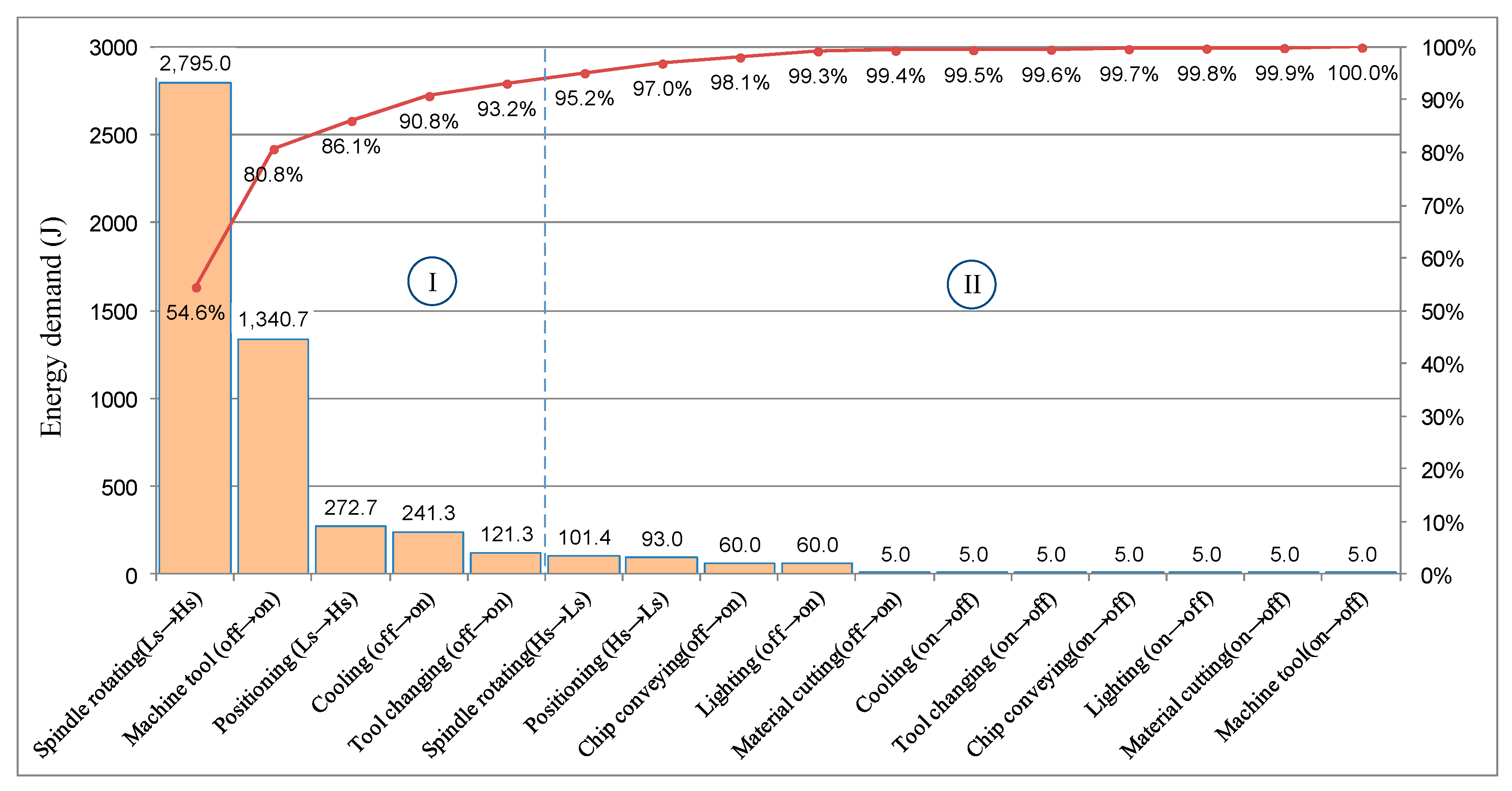
The common state transition is summarized as follows: machine tool (off→on), machine tool (on→off), lighting (off→on), lighting (on→off), cooling (off→on), cooling (on→off), chip conveying (off→on), chip conveying (on→off), spindle rotation (Ls→Hs), spindle rotation (Hs→Ls), positioning (Ls→Hs), positioning (Hs→Ls), tool changing (off→on), tool changing (on→off), material cutting (off→on), material cutting (on→off). More specifically, (off→on) indicates the state transitions from “off” mode to “on” mode; (on→off) indicates the state transitions from “on” mode to “off” mode. Similarly, (Ls→Hs) means the state transitions from “Low speed” mode to “High speed” mode; (Hs→Ls) means the state transitions from “High speed” mode to “Low speed” mode. Energy demand of each state transition is analyzed by means of experiment and the key state transitions are identified according to the Pareto principle. Taking CK6153i CNC lathe as an example, the energy demand of each state transition can be obtained by using the power and energy acquisition experimental device built by our research group [12]. The experimental device is composed of three current sensors, three voltage sensors, two NI-9215 data acquisition cards and one compact DAQ crate, etc. The experimental device is connected to the main power box of the CK6153i CNC lathe. Moreover, the power and energy information is measured and stored in the Server SQL database for offline analysis. For more information about the experimental device, you can refer to Figure 10 in Section 4. The energy demands of chip conveying (off→on) and lighting (off→on) are the estimated values because the machine tool mentioned above does not have an automatic chip conveying device and the lighting device cannot be controlled separately. In addition, because the state transition lighting/cooling/chip conveying/tool changing/machine tools (on→off) only involve instant closing of motor or lighting device, the energy demand is very low, at a value of around 5 J. The Pareto chart is obtained according to the energy demand value of each state transition gained by actual measurement, as shown in Figure 3.
According to the above Pareto chart and in accordance with the 80/20 rule, the top 20% of state transitions (top four transitions) ranked by energy demands are determined as key state transitions. The machine tool (off→on) includes three manually operated sub-movements: starting the air switch, starting the numerical control (NC) control panel, and releasing the emergency stop button. The energy demand of the machine tool (off→on) is the sum of energy demand caused by these three sub-movements. Because they are manually operated, however, the duration of the machine tool (off→on) depends on the operators. Accurate energy demand (off→on) is difficult to be obtain and therefore does not fall within the scope of this manuscript. Hence, spindle rotation (Ls→Hs), positioning (Ls→Hs), cooling (off→on) and tool changing (off→on) are finally determined to be the key state transitions (Category I), whereas other state transitions are non-key (Category II). It can be seen from the Pareto chart that the energy demand of key state transitions accounts for over 80% of the total energy demand of state transitions, thus warranting further study.
3. Methodology
3.1. Energy Demand Model of Spindle Rotation (Ls→Hs)
Spindle rotation (Ls→Hs) is the transfer process of the spindle accelerating from low speed (minimum is 0 r/min) to high speed under the conditions of non-cutting loading. Figure 4 shows the power curves of spindle rotation (Ls→Hs) (initial speed n1 = 0 r/min, the target speed n2 = 750 r/min) of CK6153i CNC lathes. Energy demand of state transition spindle rotation (Ls→Hs) includes not only energy demand of the spindle system itself, but also energy demand of supporting therbligs (standby operating, lighting, etc.) during this state transition. Energy demand of spindle rotation (Ls→Hs) consists of three parts: (1) Energy demand of spindle system from spindle rotation start to peak power (ESR1); (2) Energy demand of spindle system from peak power to stable power (ESR2); (3) Energy demand of supporting therbligs during spindle rotation (Ls→Hs) (ESR3). Thus, the energy demand of state transition of spindle rotation (Ls→Hs) is written as:
where ESRA is energy demand of spindle rotation(Ls→Hs), J.
The energy demand of the spindle system from spindle rotation start to peak power (ESR1) is calculated as:
where is the power of the spindle system from spindle rotation start to peak power, W; is duration from spindle rotation start to peak power, s.
The power of the spindle system during the acceleration process is further expressed as [33]:
The theoretical derivation process of is shown in Figure 5. Hence, the developed equation model has a certain degree of versatility.
The developed model contains some machine tool design and electrical control-related parameters (equivalent acceleration torque of spindle , etc.). However, the machine manual usually provides machine configuration-, operation- and maintenance-related information; descriptions of design and electrical control-related parameters are very limited (for technical protection reasons). Consequently, some coefficients of the developed model is difficult to be obtained without experiments, which hinder the application of the model. To make the model easier to use, the coefficients of the model (equivalent acceleration torque of spindle-, angular acceleration of spindle-, etc.) can be obtained based on the experimental studies. More specifically, each obtained coefficient value was the average value of multiple measurements. Once the coefficients of the energy model of state transitions for one machine tool are obtained, these models can be used for a long period of time. When it comes to another machine tool (of the same type of), the formula form of the energy model of state transitions can be adopted, though the coefficient values need to be updated with several simple experimental measurements.
The duration from spindle rotation start to peak power is calculated as:
where is initial spindle speed, r/min; is target spindle speed, r/min; is angular acceleration of spindle, rad/s2.
The energy demand of spindle system ESR2 from peak power to stable power is written as
where is power peak of spindle speedup, W; is the spindle power, W; is target spindle speed, r/min; is the duration from peak power to stable power, s. can be obtained based on experimental measurement combined with statistical analysis.
The power peak of spindle speedup () is spindle accelerating power at the moment (tSR1). According to Equation (3), the peak power of spindle speedup is expressed as:
The energy demand of supporting therbligs during spindle rotation (Ls→Hs) is relevant to the type and quantity of supporting therblig during state transition and the status of supporting therblig is judged by the state vector in forward-operating state [34]. The value 1 in state vector is reflected as the supporting therblig. The energy demand of supporting therbligs during spindle rotation (Ls→Hs) (ESR3) is calculated as:
where is the power vector of forward-operating state; is the state vector of forward-operating state; is the duration of spindle rotation (Ls→Hs), s. The detail explanations of Equation (7) are shown in Figure 6. are the logical representations for these eleven types of therbligs, which are represented by 0–1 variables. More specifically, when the supporting therblig is executed, then s = 1 can be obtained; otherwise, s = 0 is obtained. For instance, supposing only the therblig-standby operating and therblig-lighting are executed, then can be obtained, and are all set to be 0. As a result, the power of supporting therbligs can be expressed as: . The power model and calculation approach have been researched in our previous work [34].
The energy demand of supporting therbligs during the state transition process (ESR3) is further calculated as:
The duration of spindle rotation (Ls→Hs) is calculated as:
where is duration from spindle rotation start to peak power, s; is duration from peak power to stable power, s.
Substituting the Formulas (2)–(8) into Equation (1) to get the energy demand of spindle rotation (Ls→Hs):
3.2. Energy Demand Model of Positioning (Ls→Hs)
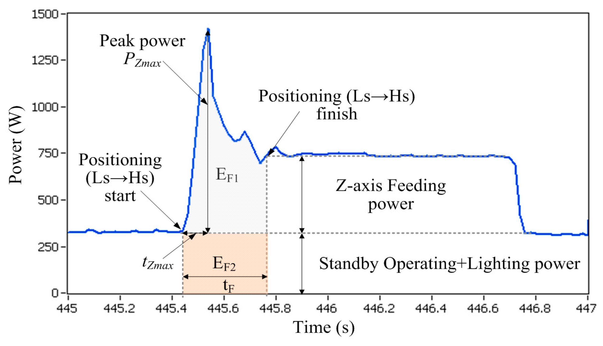
Positioning (Ls→Hs) is the transfer process of feeding system from low feeding speed (minimum is 0 r/min) to the maximum feeding speed. For a given feeding system, the maximum feed speed of each axis is definite. Taking CK6153i lathe as an example, the maximum feed speed of X-axis is 6 m/min and maximum feed speed of Z-axis is 10 m/min [35]. Figure 7 shows the power curve of Z-axis positioning (Ls→Hs) of CNC CK6153i lathe (initial feed speed vf0 = 0 mm/min, maximum feed rate vf1 = 10,000 mm/min). Similar to the state transition spindle rotation (Ls→Hs), energy demand of positioning (Ls→Hs) includes not only energy demand of the feeding system itself, but also energy demand of supporting therbligs (standby operating, lighting, etc.) during this state transition. Hence, the energy demand of positioning (Ls→Hs) consists of two parts: (1) Energy demand of feeding system during positioning (Ls→Hs) (EF1); (2) Energy demand of supporting therblig during positioning (Ls→Hs) (EF2). Thus, energy demand of positioning (Ls→Hs) is calculated as:
where is the energy demand of positioning (Ls→Hs), J.
Generally, the rapid positioning accelerations of each axis of a CNC machine is very large, some being more than 1 g [36]. Therefore, the duration of positioning (Ls→Hs) is very short, although it can cause large power peaks (corresponding to the maximum feed speed). For each feed axis, there is a critical feeding distance Lf0. When the feeding distance is Lf < Lf0, the feeding axis begins deceleration before reaching the maximum feeding speed. Because the power peak does not reach the maximum value, the duration of positioning (Ls→Hs) is very short, subsequently leading to the low energy demand in this condition. Therefore, when the feeding distance is Lf < Lf0, energy demand of positioning (Ls→Hs) is negligible. When the feeding distance is Lf ≥ Lf0, the feed axis can accelerate to the maximum speed and the corresponding power reaches a maximum power peak. Therefore, this subsection focuses on the energy demand of positioning (Ls→Hs) when feeding distance is Lf ≥ Lf0.
The critical feeding distance Lf0 can be expressed as [33]:
where is the maximum feeding speed of feed table, mm/min; is acceleration in feed table, mm/s2; is deceleration of feed table, mm/s2. can be obtained from the machine manual and can be calculated according to the machine design information.
The energy demand of feeding system during positioning (Ls→Hs) EF1 is calculated as:
where is power function of feeding system during positioning (Ls→Hs).
For a given feeding system, the maximum feeding speed and feeding acceleration of positioning (Ls→Hs) is definite, and the initial feed rate of positioning (Ls→Hs) is 0 mm/min. Hence, for each feed axis, when the feeding distance is Lf ≥ Lf0, the energy demand of feeding system EF1 and transfer time tF of positioning (Ls→Hs) are definite values, which can be obtained by experimental measurements combined with statistical analysis.
The supporting therbligs during positioning (Ls→Hs) need to be judged by the state vector in the forward-operating state [34]. The value 1 in the state vector is reflected as the supporting therblig. The energy demand of the supporting therblig (EF2) during positioning (Ls→Hs) is calculated as:
where is the duration of positioning (Ls→Hs), s.
The energy demand of positioning (Ls→Hs) is obtained by substituting the Formula (13) and (14) into Formula (11)
3.3. Energy Demand Model of Cooling (off→on)
Cooling (off→on) means the transfer process of the cooling device from “off” state to “power on” state. The energy demand of this state transition includes not only energy demand of the cooling device itself, but also energy demand of supporting therbligs (standby operating, lighting, etc.) during the state transition. Figure 8 shows a power curve of the cooling (off→on) process for the CK6153i CNC lathe. Energy demand of cooling (off→on) includes two parts: (1) Energy demand of cooling device during cooling (off→on) (ECF1); (2) Energy demand of supporting therblig during cooling (off→on) (ECF2). Therefore, the energy demand of cooling (off→on) can be calculated as:
where is the energy demand of cooling (off→on), J.
For a given CNC machine tool, energy demand of the cooling system (ECF1) and transfer time of the cooling (off→on) process (tCF) are stable values, which can be obtained by experimental measurement combined with statistical analysis.
The supporting therbligs during cooling (off→on) need to be judged by the state vector in the forward-operating state. The value 1 in the state vector is reflected as the supporting therblig. The energy demand of supporting therbligs during cooling (off→on) (ECF2) is calculated as:
where is the duration of cooling (off→on) process, s.
The energy demand of cooling (off→on) can be obtained by substituting the Formula (17) into (16).
3.4. Energy Demand Model of Tool Changing (off→on)
Tool changing (off→on) is the transfer process of a tool device changing from “off” state to “steady power” state. Figure 9 shows an actual power curve of tool changing (off→on) of CK6153i CNC lathe. It can be seen that several power peaks occur in the power curve. The reason is that the tool changing (off→on) process includes several sub-actions, such as tool changing motor rotating startup, turret rotation and motor braking. In this paper, the energy demand of tool changing (off→on) is viewed as the sum of energy demand of power peak caused by the sub-actions. Therefore, the energy demand of tool changing (off→on) can be calculated as:
where is energy demand of tool changing (off→on), J; is energy demand of power peak caused by sub-action when the rotating position number of the turret is , J; is the number of power peaks when the rotating position number of the turret is ; can be obtained by experimental measurement combined with the statistical analysis method.
Generally, the rotation method of turret of CNC lathe is the unidirectional tool changing order. Hence, the rotating position number of the turret can be calculated as:
where is the initial position of the turret; is the target position of the turret; is the total posts of the turret.
4. Case Study
4.1. Description of State Transition Cases
Case studies of spindle rotation (Ls→Hs), positioning (Ls→Hs), cooling (off→on) and tool changing (off→on) were carried out to show the feasibility of the proposed method. The state transition cases were performed on a CK6153i CNC lathe, with a spindle speed range of 30~2000 r/min, and rapid-positioning speeds of X, Z-axes at 6000, 10,000 mm/min, respectively. In order to compare the forecast energy demand of state transition with the actual energy consumption value, an energy acquisition system was set up by our research group [12]. As shown in Figure 10, the current sensor and voltage sensor are connected with the CNC machine tool to obtain the current and voltage signal and collect the real-time data through two NI-9215 data acquisition cards. The power and energy information of the CNC machine tool are obtained by using LabVIEW software before being stored in the Server SQL database. The sampling interval of the energy acquisition system was set to 0.1 s.
Based on the modeling method proposed in Section 3, case studies of six state transitions were carried out on the CK61563i CNC lathe. The determining process of experimental cases is shown in Figure 11. The principle is that the cases should cover all types of key state transitions. For the state transition spindle rotation (Ls→Hs), two conditions should be considered: initial spindle speed is zero and initial spindle speed is not zero. Therefore, spindle rotation (Ls→Hs)-[0→750 r/min] and (Ls→Hs)-[500→1000 r/min] were selected for the state transition positioning (Ls→Hs), due to the fact that only two feeding directions can be applied for the CNC lathe (X-axis and Z-axis direction). Hence, positioning-Z-axis-[0→10,000 mm/min] and positioning-X-axis [0→6000 mm/min] were selected as experimental cases. For the state transition cooling (off→on), only one condition should be considered: cooling device is transiting from “off” state to “on” state (cooling (off→on) was selected). For the state transition tool changing (off→on), the cutting tool changes from one position of the turret to another. The most commonly used changing was selected: tool changing (off→on)-[Tpi = 1, Tpt = 2].
The above-mentioned six cases cover all the four type of key state transitions, and the main parameters of the above cases are shown in Table 1.
Taking spindle rotation (Ls→Hs)-[500→1000 r/min] as an example, coefficients TS and α of the AH transmission chain can be obtained according to spindle startup experiment (TS = 28.42 N·m, α = 39.78 rad/s2) [33]. The coefficient values are substituted into (3) and (4) to obtain the expressions of the spindle speedup power and the duration from spindle rotation start to peak power for the researched CK61563i CNC lathe.
The duration from peak power to stable power is related to the target spindle speed . Based on the measured at different target spindle speeds (see Table 2), linear regression between and is conducted (as shown in Figure 12) to establish the duration model from peak power to stable power (Equation (23)).
The correlation coefficient is R2 = 0.9479, which indicates that the established model can well describe under different target spindle speeds.
Taking spindle rotation (Ls→Hs) as an example, the known information is the initial speed r/min and target speed r/min. Based on the proposed method in Section 3.1, the energy demand of spindle rotation (Ls→Hs)-[0→750 r/min] () can be calculated, as shown in Figure 13. The input data, reference equations and calculation results of intermediate variables are clearly shown in this figure.
Similarly, energy demands of the other five state transitions can also be computed according to the established models in Section 3. The obtained energy demands of state transitions-spindle rotation (Ls→Hs)-[0→750 r/min], state transitions-spindle rotation (Ls→Hs)-[500→1000 r/min], positioning (Ls→Hs)-[Z-axis], positioning (Ls→Hs)-[X-axis], cooling (off→on) and tool changing (off→on) are 4078.6 J, 5056.8 J, 277.5 J, 117.2 J, 241.3 J and 116.8 J, respectively.
4.2. Discussion
By using the energy acquisition system shown in Figure 10, the actual energy consumptions of these six state transitions were measured. The predicted energy demand values of these six state transitions are compared to the measured energy values, as shown in Figure 14. It can be seen that most predictive accuracies of the state transition cases are above 90%, which shows that the proposed energy demand models of key state transitions can well describe the energy consumption behaviors of the state transitions of turning processes.
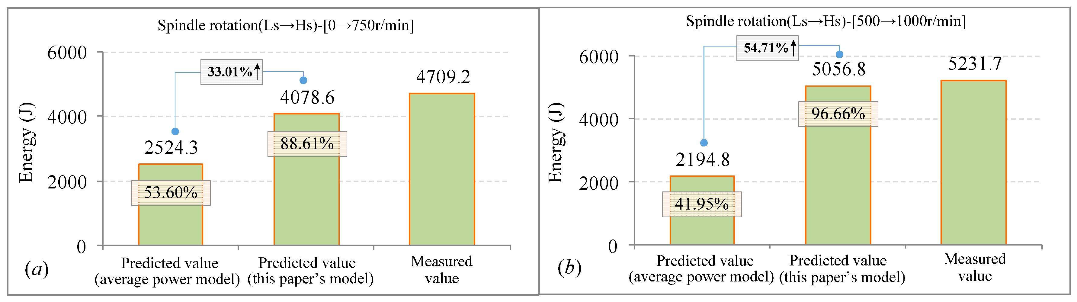
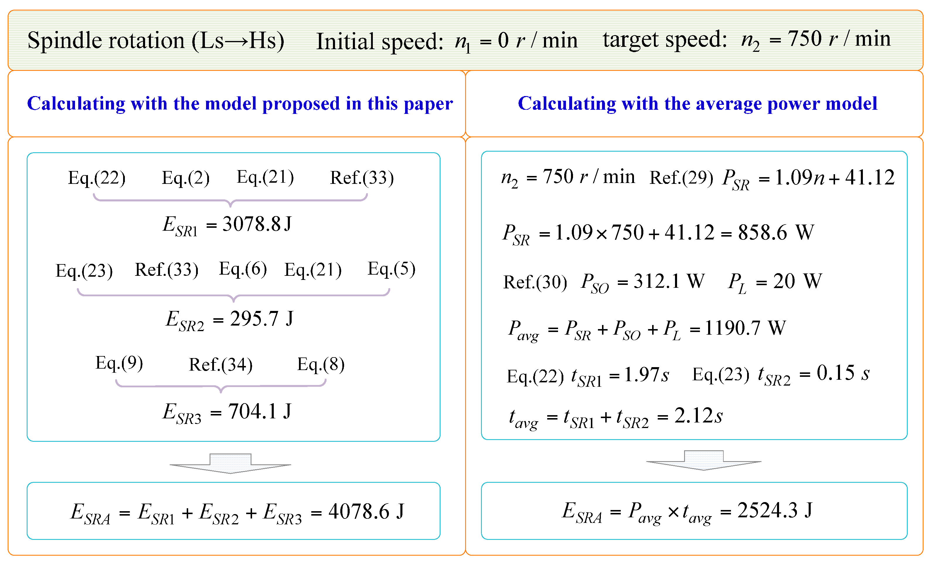
For the state transition spindle rotation (Ls→Hs), sometimes average machining power of state transition was used to calculate the energy consumption during state transition. Compared to the model without considering the energy demand of state transitions, the accuracy can be improved to a certain extent via applying the average machining power of state transitions. However, the accuracy of the average power model is not optimistic as this is a simplistic model. The energy demand models proposed in this paper can further improve the energy predictive accuracy of the state transitions compared with the average power model. Taking the state transition spindle rotation (Ls→Hs)-[0→750 r/min] of CK6153i as an example, the energy demand of spindle (Ls→Hs)-[0→750 r/min] has been obtained based on the proposed model in this paper by the aforementioned calculating processes: J ( briefly shown in Figure 15). Moreover, if the average power model is used to predict energy consumption, the calculating process and result is also shown in Figure 15. It can be seen that the energy demand of the state transition spindle rotation (Ls→Hs)-[0→750 r/min] calculated by using the average power model is J. Similarly, predicted energy values with the average power model and this paper’s model can be calculated from the state transition spindle rotation (Ls→Hs)-[500→1000 r/min]. The comparison of the predicted energy values with these two models for the state transition spindle rotation (Ls→Hs) is shown in Figure 16.
It can be seen from Figure 16a that the predicted energy value with the average power model for the state transition spindle rotation (Ls→Hs)-[0→750 r/min] is 2524.3 J (the actual measured energy value is 4709.2 J); the predictive accuracy is thus only 53.60% when using the average power model. When it comes to the state transition spindle rotation (Ls→Hs)-[500→1000 r/min], the predictive accuracy is also not satisfactory (41.95%). The reason is that the power during state transition is treated as a single value in the average power model and the dynamic power change and power peak were not considered. Indeed, the average power is far less than the peak power of the state transition, particularly in the state transition spindle rotation (Ls→Hs). With the proposed method in this paper, the predicted energy value for the state transition spindle rotation (Ls→Hs)-[0→750 r/min] is 4078.6 J. Hence, the predictive accuracy is 88.61%, improving the accuracy by 33.01% compared with the average power model. A similar result is also obtained in the case of the state transition spindle rotation (Ls→Hs)-[500→1000 r/min]. The predictive accuracy is raised from 41.95% to 96.66%, i.e., 54.71% improvement is achieved. The results show that the energy demand model proposed in this paper can further improve the energy-predictive accuracy of the state transitions compared with the average power model.
5. Conclusions
State transitions occur frequently during the turning process, and energy demand of the machining state transition is an important part of that entire process. The establishment of energy demand models of the key state transitions could significantly improve the accuracy of a turning process energy model. The state transitions are classified according to energy characteristics, and the key state transitions for turning processes are identified. Then, the energy demand model of four types of key state transitions are respectively researched and established. Finally, experimental studies and case studies are performed on a CK6153i CNC lathe, the results showing that predictive accuracy with the proposed method is generally above 90% for the state transition cases. In particular, the predictive accuracy can be improved by 33.01% and 54.71% for the two state transition cases (spindle rotations (Ls→Hs)-[0→750 r/min] and (Ls→Hs)-[500→1000 r/min]) compared with the average power model. The proposed method in this paper can provide more accurate energy models and reliable data of state transitions for energy optimization of turning processes.
Although this study presents energy demand modeling of key state transitions of the turning process, the dynamic distribution of key state transitions and total energy demand of state transitions throughout the machining process have not yet been investigated. Further research will be carried out to analyze key state transition distribution during the machining process and propose an energy demand modeling method of state transitions for all stages of the machining process.
Acknowledgments
The authors sincerely thank editors and anonymous reviewers for their helpful suggestions on the quality improvement of our paper. This research is supported by the Shandong Provincial Natural Science Foundation, China (No. ZR2016GQ11), Scientific Research Foundation of Shandong University of Science and Technology for Recruited Talents (No. 2015RCJJ049).
Author Contributions
Qinghe Yuan and Dawei Ren proposed the paper structure, Shun Jia and Jingxiang Lv designed and performed the experiments. Shun Jia conceived the paper, analyzed the data and wrote the paper.
Conflicts of Interest
The authors declare no conflict of interest.
Nomenclature
| acceleration in feed table (mm/s2) | |
| depth of cut (mm) | |
| deceleration of feed table (mm/s2) | |
| energy demand of cooling (off→on) (J) | |
| energy demand of cooling device during cooling (off→on) (J) | |
| energy demand of supporting therblig during(off→on) (J) | |
| energy demand of positioning (Ls→Hs) (J) | |
| energy demand of feeding system during positioning (Ls→Hs) (J) | |
| energy demand of supporting therblig during positioning (Ls→Hs) (J) | |
| energy demand of spindle rotation (Ls→Hs) (J) | |
| energy demand of spindle system from spindle rotation start to peak power (J) | |
| energy demand of spindle system from peak power to stable power (J) | |
| energy demand of supporting therbligs during spindle rotation (Ls→Hs) (J) | |
| energy demand of tool changing (off→on) (J) | |
| energy demand of power peak caused by sub-action k when the rotating position number of the turret is (J) | |
| IEA | International Energy Agency |
| number of power peak when the rotating position number of the turret is | |
| feeding distance (mm) | |
| critical feeding distance (mm) | |
| LCA | Life Cycle Analysis |
| spindle speed (r/min) | |
| initial spindle speed (r/min) | |
| target spindle speed (r/min) | |
| power vector of forward-operating state | |
| state vector of forward-operating state | |
| power of therblig-chip conveying (W) | |
| power of therblig-cutting flood spraying (W) | |
| power function of feeding system during positioning (Ls→Hs) | |
| power of therblig- lighting (W) | |
| power of therblig- material cutting (W) | |
| power of therblig-standby operating (W) | |
| spindle power (W) | |
| power of spindle system from spindle rotation start to peak power (W) | |
| power peak of spindle speedup (W) | |
| power of therblig-tool changing (W) | |
| power of therblig-tool selecting (W) | |
| power of therblig-X-axis feeding (W) | |
| power of therblig-Y-axis feeding (W) | |
| power of therblig-Z-axis feeding (W) | |
| logical representations for ith type of therbligs | |
| transfer time of cooling (off→on) process (s) | |
| transfer time of positioning (Ls→Hs) (s) | |
| duration from spindle rotation start to peak power (s) | |
| duration from peak power to stable power (s) | |
| duration of spindle rotation (Ls→Hs) (s) | |
| total posts of the turret | |
| initial position of the turret | |
| target position of the turret | |
| equivalent acceleration torque of spindle (N·m) | |
| initial feed speed (mm/min) | |
| maximum feed rate (mm/min) | |
| maximum feeding speed of feed table (mm/min) | |
| angular acceleration of spindle (rad/s2) | |
| angular velocity of spindle rotation (rad/s) | |
| rotating position number of the turret |
References
- International Energy Agency. Energy Technology Perspectives 2010: Scenarios and Strategies to 2050; International Energy Agency: Paris, France, 2010. [Google Scholar]
- Wei, W.; Liang, Y.; Liu, F.; Mei, S.; Tian, F. Taxing strategies for carbon emissions: A bilevel optimization approach. Energies 2014, 7, 2228–2245. [Google Scholar] [CrossRef]
- Thollander, P.; Palm, J. Industrial energy management decision making for improved energy efficiency—Strategic system perspectives and situated action in combination. Energies 2015, 8, 5694–7703. [Google Scholar] [CrossRef]
- Anderberg, S.E.; Kara, S.; Beno, T. Impact of energy efficiency on computer numerically controlled machining. Proc. Inst. Mech. Eng. B J. Eng. 2010, 224, 531–541. [Google Scholar] [CrossRef]
- Brown, N.; Greenough, R.; Vikhorev, K.; Khattack, S. Precursor to using energy data as a manufacturing process variable. In Proceedings of the 6th IEEE International Conference on Digital Ecosystems Technologies (DEST), Campione d’Italia, Italy, 18–20 June 2012. [Google Scholar]
- Shao, G.; Kibira, D.; Lyons, K. A virtual machining model for sustainability analysis. In Proceedings of the ASME 2010 International Design Engineering Technical Conferences & Computers and Information in Engineering Conference, Montreal, QC, Canada, 15–18 August 2010. [Google Scholar]
- Zulaika, J.J.; Dietmair, A.; Campa, F.J.; López de Lacalle, L.N.; Verbeeten, W. Eco-efficient and Highly Productive Production Machines by Means of a Holistic Eco-Design Approach. In Proceedings of the 3rd Conference on Eco-Efficiency, Egmond an Zee, The Netherlands, 9–11 June 2010. [Google Scholar]
- Salonitis, K. Energy efficiency assessment of grinding strategy. Int. J. Energy Sect. Manag. 2015, 9, 20–37. [Google Scholar] [CrossRef]
- Salonitis, K.; Vidon, B.; Chen, D. A decision support tool for the energy efficient selection of process plans. Int. J. Mech. Manuf. Syst. 2015, 8, 63–83. [Google Scholar] [CrossRef]
- Gutowski, T. Energy and Environmental Issues for Manufacturing Processes. Available online: http://web.mit.edu/2.810/www/lecture2011/Environment.pdf (accessed on 27 August 2011).
- Gutowski, T.; Dahmus, J.; Thiriez, A. Electrical energy requirements for manufacturing processes. In Proceedings of the 13th CIRP International Conference on Life Cycle Engineering, Leuven, Belgium, 31 May–2 June 2006. [Google Scholar]
- Jia, S.; Tang, R.Z.; Lv, J.X. Therblig-based energy demand modeling methodology of machining process to support intelligent manufacturing. J. Intell. Manuf. 2014, 25, 913–931. [Google Scholar] [CrossRef]
- Lv, J.X.; Tang, R.Z.; Jia, S. Therblig-based energy supply modeling of CNC machine tools. J. Clean. Prod. 2014, 65, 168–177. [Google Scholar] [CrossRef]
- Li, W.; Kara, S. An empirical model for predicting energy consumption of manufacturing processes: A case of turning process. Proc. Inst. Mech. Eng. B J. Eng. 2011, 225, 1636–1646. [Google Scholar] [CrossRef]
- Balogun, V.A.; Mativenga, P.T. Modeling of direct energy requirements in mechanical machining processes. J. Clean. Prod. 2013, 41, 179–186. [Google Scholar] [CrossRef]
- Jia, S.; Tang, R.Z.; Lv, J.X.; Zhang, Z.W.; Yuan, Q.H. Energy modeling for variable material removal rate machining process: An end face turning case. Int. J. Adv. Manuf. Technol. 2016, 85, 2805–2818. [Google Scholar] [CrossRef]
- Zobel, T.; Malmgren, C. Evaluating the management system approach for industrial energy efficiency improvements. Energies 2016, 9, 774. [Google Scholar] [CrossRef]
- Tan, X.C.; Wang, Y.Y.; Gu, B.H.; Mu, Z.K.; Yang, C. Improved methods for production manufacturing processes in environmentally benign Manufacturing. Energies 2011, 4, 1391–1409. [Google Scholar] [CrossRef]
- Chiu, T.-Y.; Lo, S.-L.; Tsai, Y.-Y. Establishing an integration-energy-practice model for improving energy performance Indicators in ISO 50001 energy management systems. Energies 2012, 5, 5324–5339. [Google Scholar] [CrossRef]
- Peng, T.; Xu, X. Energy-efficient machining systems: A critical review. Int. J. Adv. Manuf. Technol. 2014, 72, 1389–1406. [Google Scholar] [CrossRef]
- Salonitis, K.; Ball, P. Energy efficient manufacturing from machine tools to manufacturing systems. Procedia CIRP 2013, 7, 634–639. [Google Scholar] [CrossRef]
- Salonitis, K.; Zeng, B.; Mehrabi, H.A.; Jolly, M.R. The challenges for energy efficiency casting processes. Procedia CIRP 2016, 40, 24–29. [Google Scholar] [CrossRef]
- Domingo, R.; Marín, M.; Claver, J.; Calvo, R. Selection of cutting inserts in dry machining for reducing energy consumption and CO2 emissions. Energies 2015, 8, 13081–13095. [Google Scholar] [CrossRef]
- Zhai, Q.; Cao, H.; Zhao, X.; Yuan, C. Cost benefit analysis of using clean energy supplies to reduce greenhouse gas emissions of global automotive manufacturing. Energies 2011, 4, 1478–1494. [Google Scholar] [CrossRef]
- Campatelli, G.; Lorenzini, L.; Scippa, A. Optimization of process parameters using a Response Surface Method for minimizing power consumption in the milling of carbon steel. J. Clean. Prod. 2014, 66, 309–316. [Google Scholar] [CrossRef]
- Santos, J.P.; Oliveira, M.; Almeida, F.G.; Pereira, J.P.; Reis, A. Improving the environmental performance of machine-tools: Influence of technology and throughput on the electrical energy consumption of a press-brake. J. Clean. Prod. 2011, 19, 356–364. [Google Scholar] [CrossRef]
- Herrmann, C.; Thiede, S. Process chain simulation to foster energy efficiency in manufacturing. CIRP J. Manuf. Sci. Technol. 2009, 1, 221–229. [Google Scholar] [CrossRef]
- Abele, E.; Sielaff, T.; Schiffler, A.; Rothenbücher, S. Analyzing energy consumption of machine tool spindle units and identification of potential for improvements of efficiency. In Proceedings of the 18th CIRP International Conference on Life Cycle Engineering, Braunschweig, Germany, 2–4 May 2011. [Google Scholar]
- He, Y.; Liu, F.; Wu, T.; Zhong, F.; Peng, B. Analysis and estimation of energy consumption for numerical control machining. Proc. Inst. Mech. Eng. B J. Eng. 2011, 226, 255–266. [Google Scholar] [CrossRef]
- Reinhart, G.; Reinhardt, S.; Föckerer, T.; Zäh, M.F. Comparison of the Resource Efficiency of Alternative Process Chains for Surface Hardening. In Proceedings of the 18th CIRP International Conference on LCE, Braunschweig, Germany, 2–4 May 2011. [Google Scholar]
- Avram, O.I.; Xirouchakis, P. Evaluating the use phase energy requirements of a machine tool system. J. Clean. Prod. 2011, 19, 699–711. [Google Scholar] [CrossRef]
- Shi, J.L.; Liu, F.; Xu, D.J.; Chen, G.R. Decision model and practical method of energy-saving in NC machine tool. China Mech. Eng. 2009, 20, 1344–1346. [Google Scholar]
- Lv, J.X. Research on Energy Supply Modeling of Computer Numerical Control Machine Tools for Low Carbon Manufacturing. Ph.D. Thesis, Zhejiang University, Hangzhou, China, 2014. [Google Scholar]
- Jia, S. Research on Energy Demand Modeling and Intelligent Computing of Machining Process for Low Carbon Manufacturing. Ph.D. Thesis, Zhejiang University, Hangzhou, China, 2014. [Google Scholar]
- CK6153i Series. Manual Specification of CK6153i Series CNC Lathe; Jinan First Machine Tool Group Co., Ltd. of China: Jinan, China, 2000. [Google Scholar]
- China Commodity Net. Technological Development and Gap of Domestic CNC Machine Tools. Available online: http://ccn.mofcom.gov.cn/spbg/show.php?id=12952 (accessed on 26 April 2012).
Figure 1.
Power curve during an actual machining process [25].
Figure 1.
Power curve during an actual machining process [25].
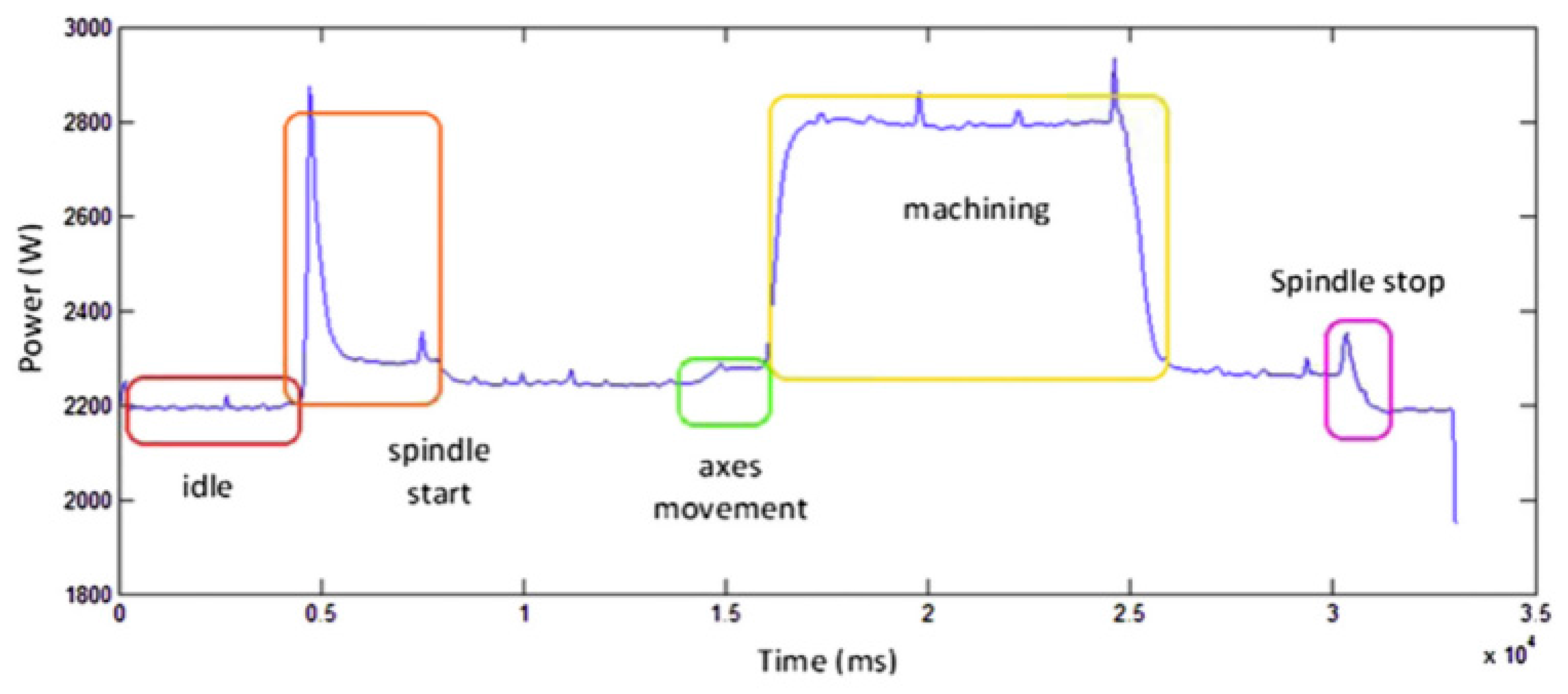
Figure 2.
Framework of the proposed methodology.
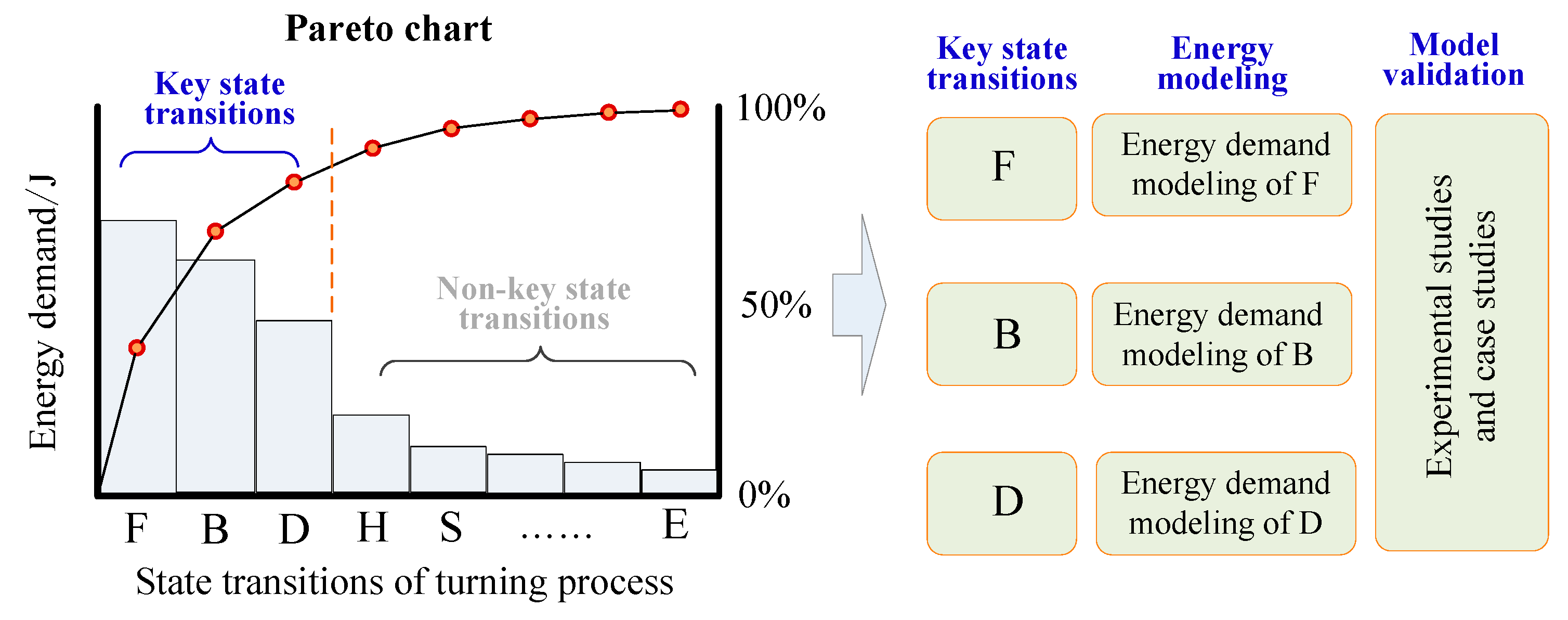
Figure 3.
Pareto chart during an actual turning process.

Figure 4.
Power curve of spindle rotation (Ls→Hs).
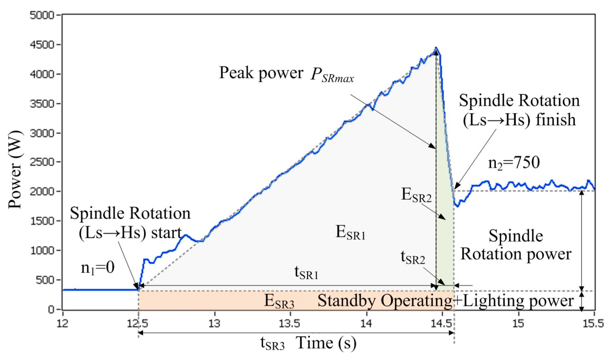
Figure 5.
Theoretical derivation process of .
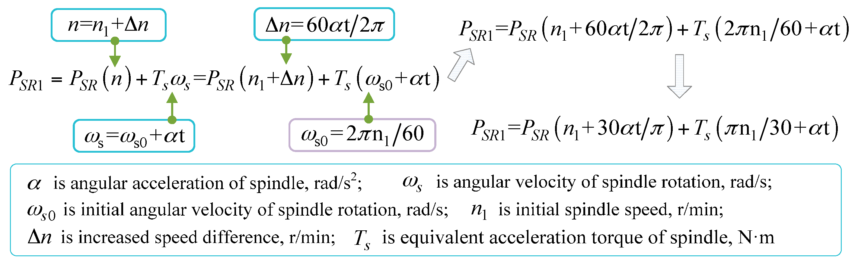
Figure 6.
Detail explanations of Equation (7).
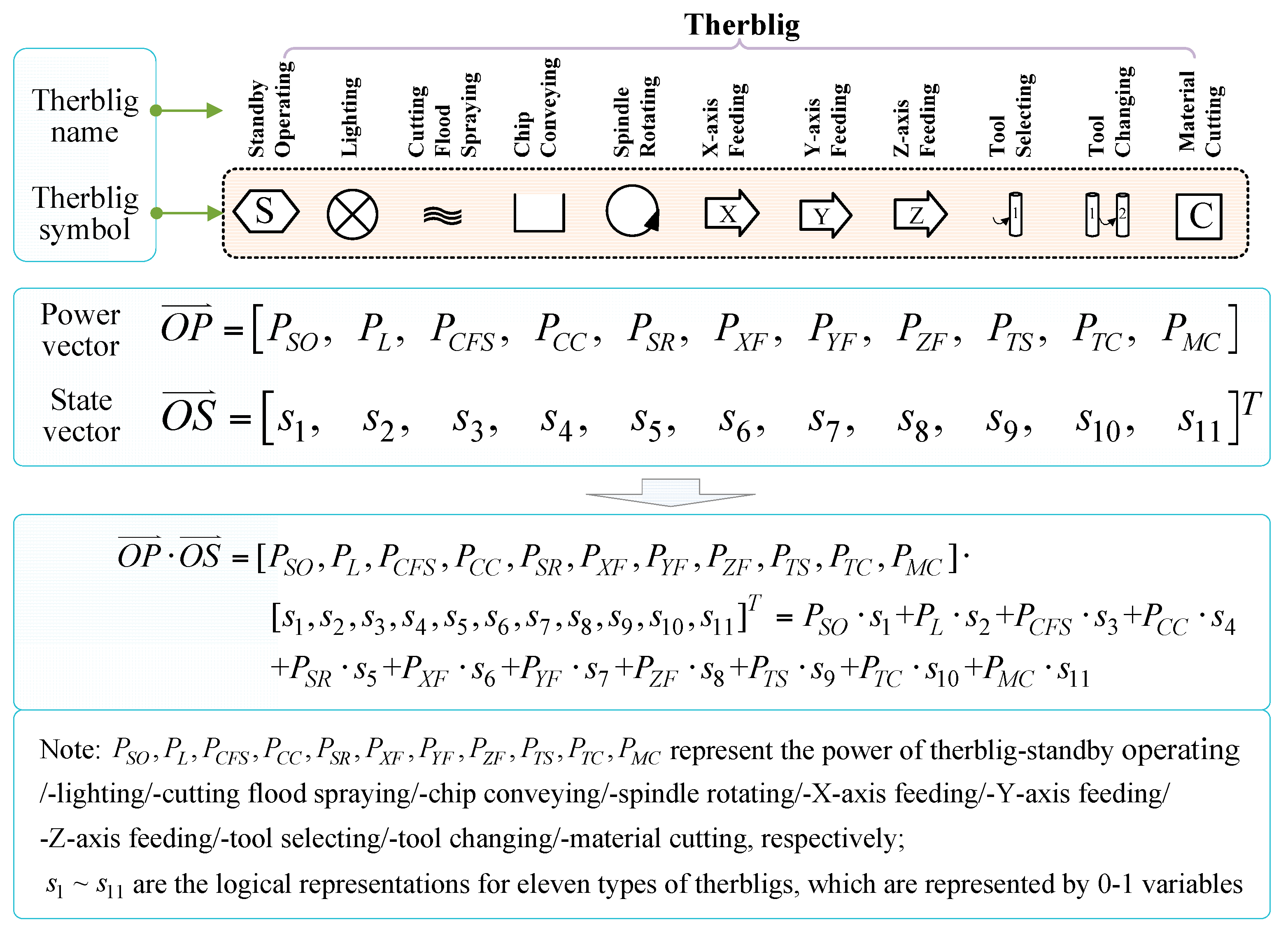
Figure 7.
Power curve of positioning (Ls→Hs).

Figure 8.
Power curve of cooling (off→on).

Figure 9.
Power curve of tool changing (off→on).

Figure 10.
Experimental setup of energy acquisition system.
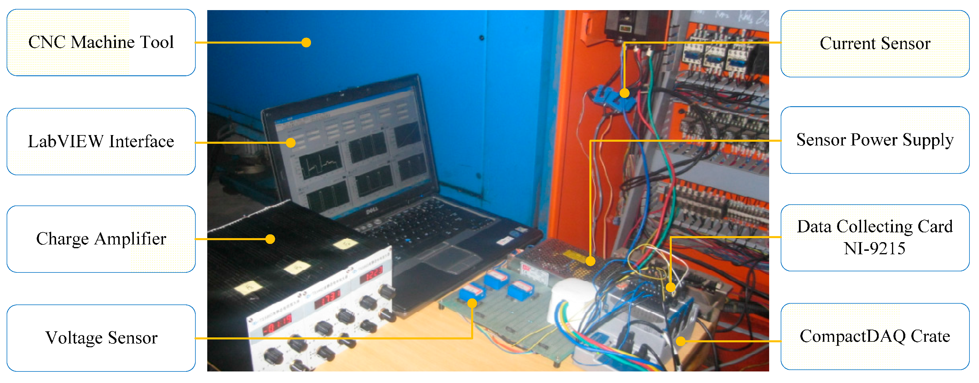
Figure 11.
Determining process of experimental cases.
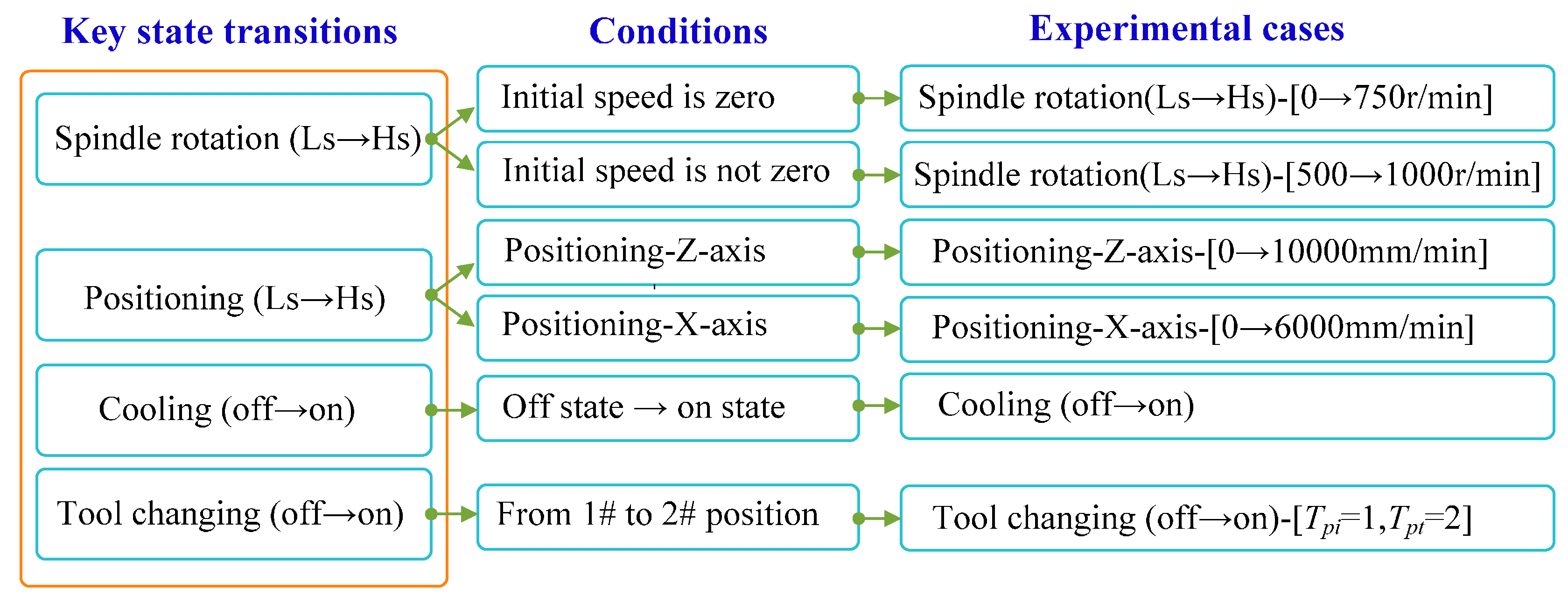
Figure 12.
Linear fitting between tSR2 and n2.
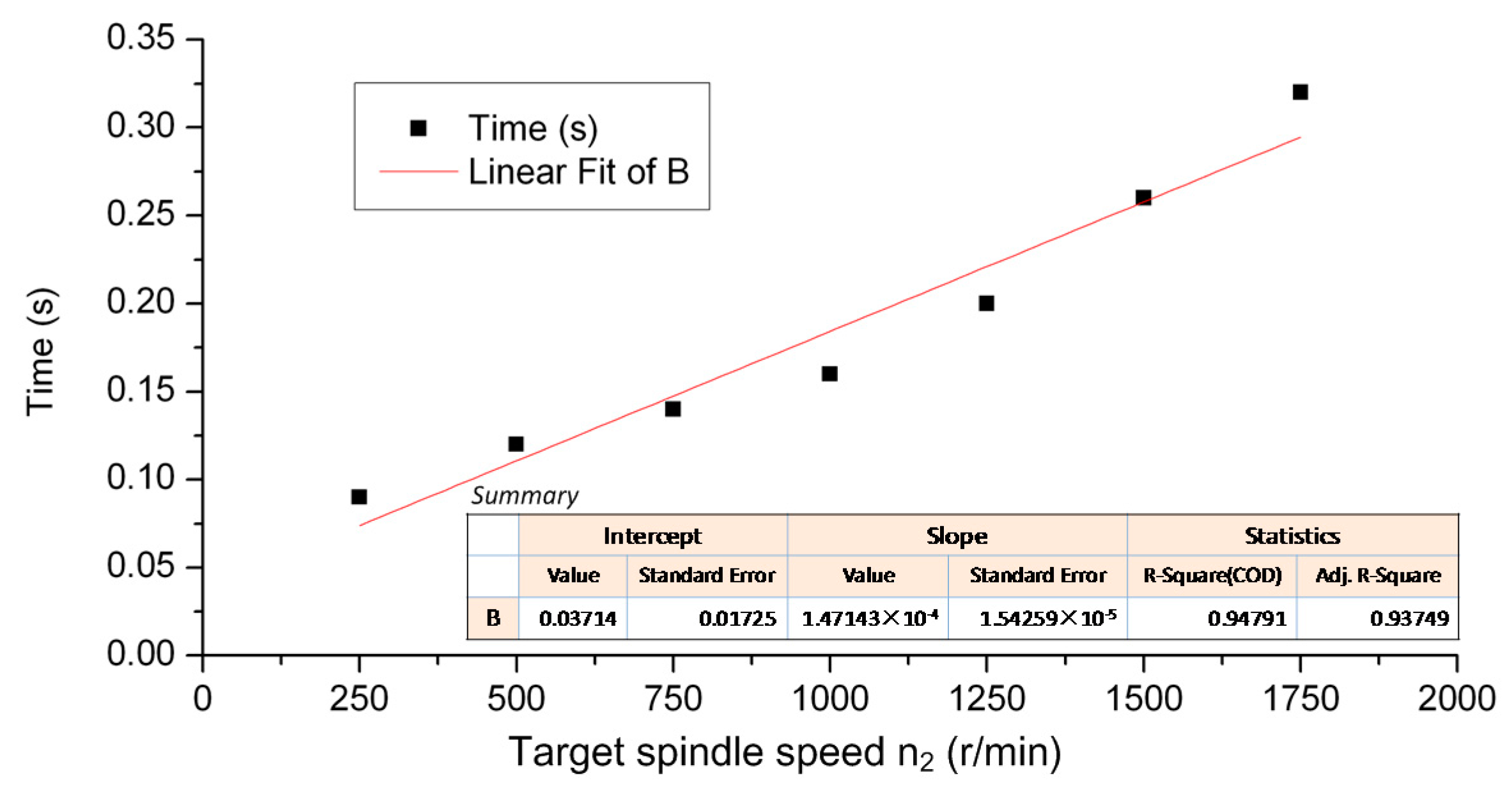
Figure 13.
Calculation process of energy demand of spindle rotation (Ls→Hs)-[0→750 r/min].
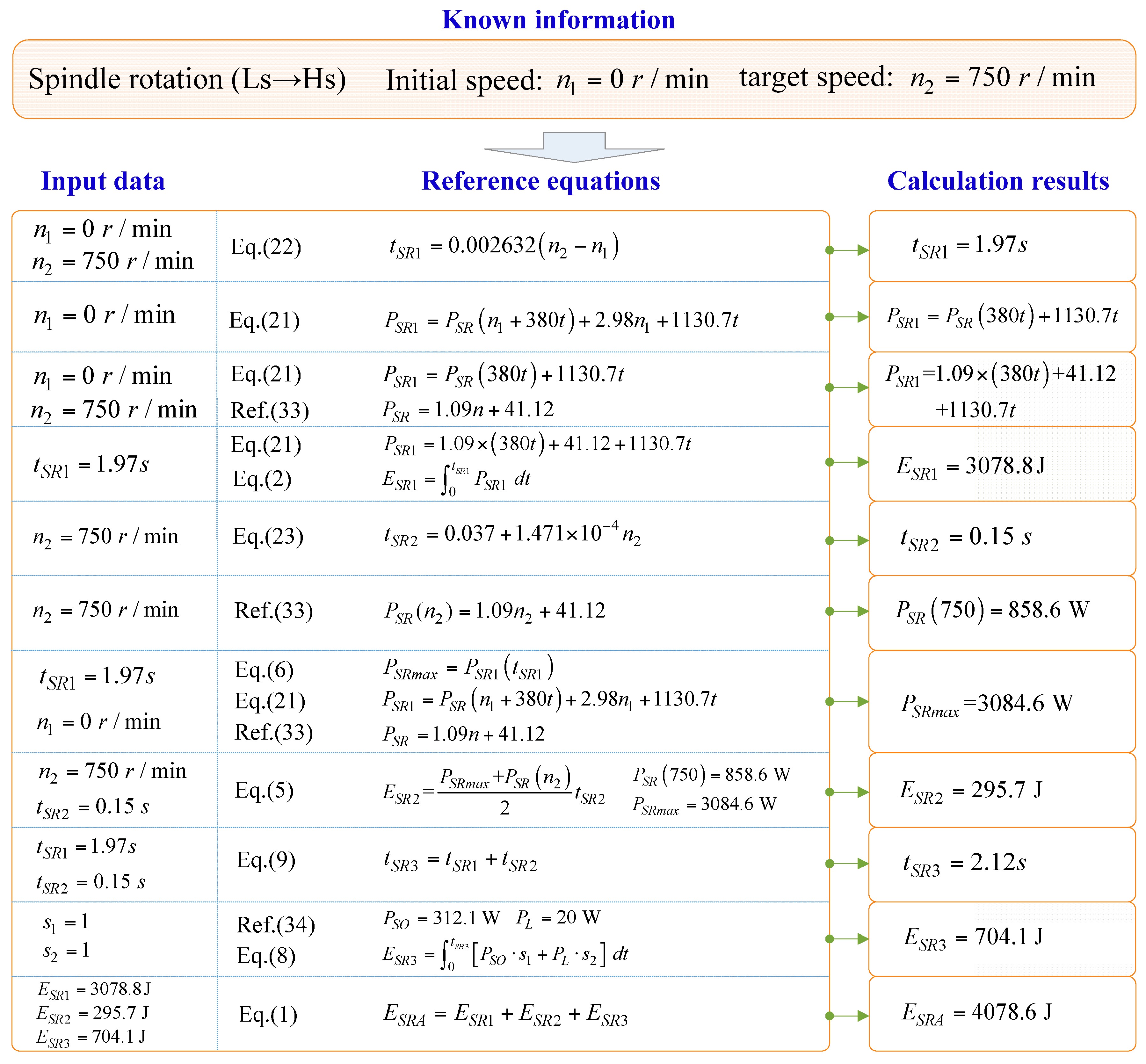
Figure 14.
Predicted energy values vs. measured values of state transitions.
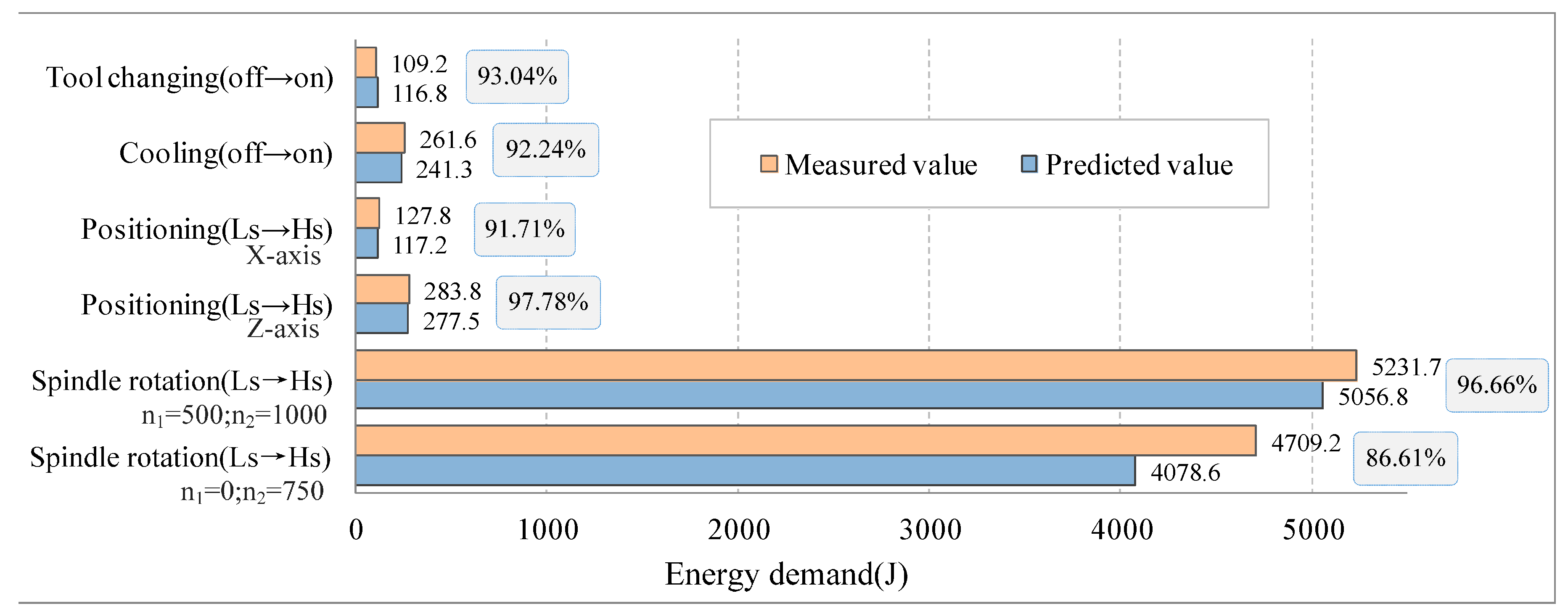
Figure 15.
Energy demand calculated with the model proposed in this paper and the average power model.
Figure 15.
Energy demand calculated with the model proposed in this paper and the average power model.

Figure 16.
Comparison of predicted values and measured values for (a) spindle rotation (Ls→Hs)-[0→750 r/min] and (b) spindle rotation (Ls→Hs)-[500→1000 r/min].
Figure 16.
Comparison of predicted values and measured values for (a) spindle rotation (Ls→Hs)-[0→750 r/min] and (b) spindle rotation (Ls→Hs)-[500→1000 r/min].

Table 1.
Main parameters of state transition cases.
| State Transition | Main Parameters | ||
|---|---|---|---|
| Initial Parameter | Target Parameter | Supporting Therbligs | |
| Spindle rotation (Ls→Hs) 0→750 r/min | n1 = 0 r/min | n2 = 750 r/min | standby operating/lighting |
| Spindle rotation (Ls→Hs) 500→1000 r/min | n1 = 500 r/min | n2 = 1000 r/min | standby operating/lighting |
| Positioning (Ls→Hs) Z-axis | vrmin = 0 mm/min | vrmax = 10,000 mm/min | standby operating/lighting |
| Positioning (Ls→Hs) X-axis | vrmin = 0 mm/min | vrmax = 6000 mm/min | standby operating/lighting |
| Cooling (off→on) | Off state | On state | standby operating/lighting |
| Tool changing (off→on) | Tpi = 1 | Tpt = 2 | standby operating/lighting |
Table 2.
Duration from peak power to stable power (tSR2) under different target spindle speeds.
| Target Spindle Speed n2 (r/min) | tSR2 (s) |
|---|---|
| 250 | 0.09 |
| 500 | 0.12 |
| 750 | 0.14 |
| 1000 | 0.16 |
| 1250 | 0.20 |
| 1500 | 0.26 |
| 1750 | 0.32 |
© 2017 by the authors. Licensee MDPI, Basel, Switzerland. This article is an open access article distributed under the terms and conditions of the Creative Commons Attribution (CC BY) license (http://creativecommons.org/licenses/by/4.0/).
Share and Cite
MDPI and ACS Style
Jia, S.; Yuan, Q.; Ren, D.; Lv, J. Energy Demand Modeling Methodology of Key State Transitions of Turning Processes. Energies 2017, 10, 462. https://doi.org/10.3390/en10040462
AMA Style
Jia S, Yuan Q, Ren D, Lv J. Energy Demand Modeling Methodology of Key State Transitions of Turning Processes. Energies. 2017; 10(4):462. https://doi.org/10.3390/en10040462
Chicago/Turabian StyleJia, Shun, Qinghe Yuan, Dawei Ren, and Jingxiang Lv. 2017. "Energy Demand Modeling Methodology of Key State Transitions of Turning Processes" Energies 10, no. 4: 462. https://doi.org/10.3390/en10040462
Note that from the first issue of 2016, this journal uses article numbers instead of page numbers. See further details here.