
Methodology Applied to the Evaluation of Natural Ventilation in Residential Building Retrofits: A Case Study


GIR Arquitectura & Energía, Universidad de Valladolid, ETS Arquitectura, Valladolid 47014, Spain
*
Author to whom correspondence should be addressed.
Energies 2017, 10(4), 456; https://doi.org/10.3390/en10040456
Submission received: 22 December 2016
/
Revised: 11 March 2017
/
Accepted: 18 March 2017
/
Published: 1 April 2017
(This article belongs to the Special Issue Energy Conservation in Infrastructures 2016)
Abstract
:The primary objective of this paper is to present the use of a steady model that is able to qualify and quantify available natural ventilation flows applied to the energy retrofitting of urban residential districts. In terms of air quality, natural ventilation presents more efficient solutions compared to active systems. This method combines numeric simulations, through the utilization of Ansys Fluent R15.0® and Engineering Equation Solver EES®, with on-site pressurization tests. Testing consists of the application of the seasonal pressure gradient on the building’s envelope and the calculation of the ventilation flows in three climatic representative conditions (summer, winter, and annual average). Through the implementation of this methodology to existing buildings it is possible to evaluate the influence of the built environment, as well as key parameters (relative height of the dwelling, number of vertical ventilation ducts, and airtightness of windows) of available natural ventilation.
1. Introduction
Natural ventilation of buildings is unanimously considered as a strategy for energy-efficient ventilation. Many advantages are derived from this historical tradition, such as lower costs compared to other systems and minimal maintenance [1].
The greatest limitation to natural ventilation is its dependence on climate factors, which, depending on the circumstances, may cause spaces inside to be inadequately ventilated. An uncontrolled air exchange regime arises, which must be avoided [2]. This lack of control forces the designer to opt for mechanical systems, using fans to ensure continuous air flow into dwellings, instead of using the available natural source. A strategy focused on efficient systems prompts us to maximize the use of natural ventilation, with an air support system if necessary (‘hybrid ventilation’) [3]. For this, it is necessary to qualify and quantify the availability of natural ventilation flows within the residential building being retrofitted.
Although natural ventilation lost importance in buildings in the mid-20th century, there is great research potential; present research lines have been developed by previous researchers. Current lines study the significant energy savings in most weather conditions [4], with respect to traditional mechanical exhaust systems [5], in different urban environments [6], occupancy profiles [7] and the ability to apply this strategy in building retrofits [8]. As for the influence on thermal comfort and indoor air quality, natural ventilation provides thermal control [9], free cooling [10] and contaminant removal benefits [11]. Finally, it is necessary to review the multiple configurations of building façades [12] and available conditioning devices [13,14].
The main objective of this paper is to present the use of a steady model able to both qualify and quantify available natural ventilation flows applied to the energy retrofitting of urban residential districts.
2. Area of Interest
In general, building retrofitting has significantly grown in importance in recent years as a result of an increased awareness for protecting the legacy of urban centers. As a result, public administrations have promoted this process through economic incentives designed to improve energy and comfort conditions.
The CITyFiED (RepliCable and InnovaTive Future Efficient Districts and cities) project [15], co-funded by the VII Framework Programme of the EU under Grant Agreement No. 609129, has the purpose of developing a strategy focused on 20-20-20 objectives, based on the development and implementation of innovative technologies and methodologies to renovate buildings. The project includes the comprehensive retrofitting of three large urban districts in Laguna de Duero-Valladolid (Spain), Soma (Turkey) and Lund (Sweden).
The intervention in Laguna de Duero involves retrofitting the Torrelago district, made up of eight groups of residential blocks (31 buildings with a total of 1488 dwellings) built between 1977 and 1981. The built environment close to the intervention area has been classified. The obtained classification allows definition of the roughness of the ground boundary roughness, which is used to set the boundary conditions for the inlet surface. The urban development is in an interface region between suburban and urban areas, enabling us to identify four environments (Figure 1):
- Type 1: A structured urban area to the east of the development, with residential blocks of five and six stories, separated by urban corridors.
- Type 2: A low-density and low-height environment combined with green spaces.
- Type 3: A medium-density area with alternating blocks of two- and three-story buildings and attached single family units.
- Type 4: A rural environment, with limited wooded areas and a lake that lends its name to the town.
Each building has 12 stories, with four apartments per floor and a total project surface area of 140,000 m2 to be retrofitted in two phases during the 2014–2017 period. There are three types of H-shaped buildings, called Blocks A, B and C, with two types of apartment layouts. The smaller layout has three bedrooms (3BR), a living area, a kitchen and two bathrooms, all of which have openings in their façades. The larger layout has four bedrooms (4BR), a living area, a kitchen and two bathrooms, all of which have openings in their façades, except for one of the bathrooms, which is internal. Block A has four small apartments per floor, Block C has four large apartments per floor and Block B has two small and two large apartments per floor (Figure 2).
With respect to air quality, in the original project, only natural ventilation is available. Therefore, all of the rooms have exterior framed openings and certain damp areas (kitchens and indoor baths) have a shunt type shared shaft that leads to the roof. However, these shafts are not always reliable because successive interventions by owners have obstructed or eliminated many of them.
3. Methodology
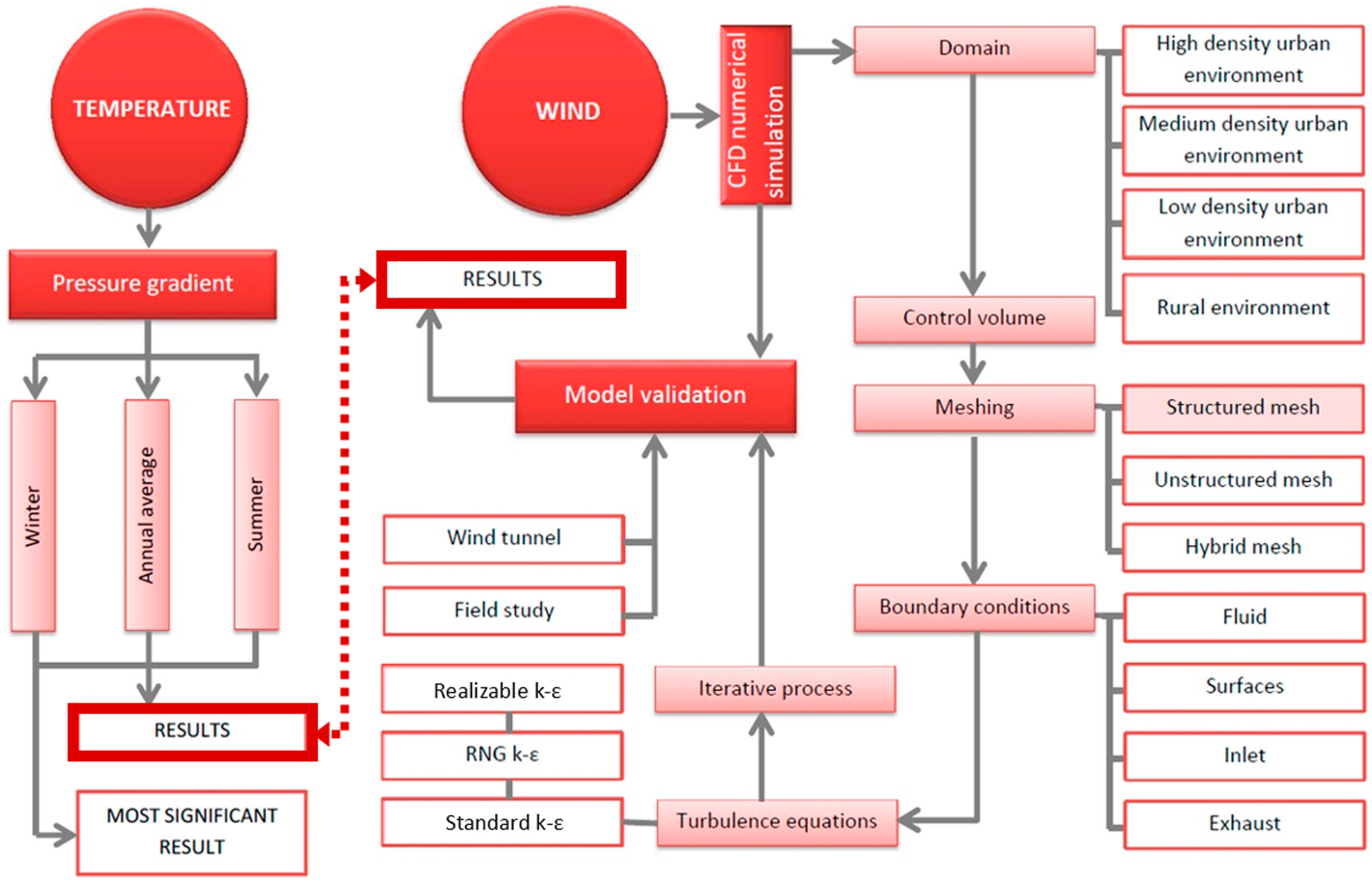
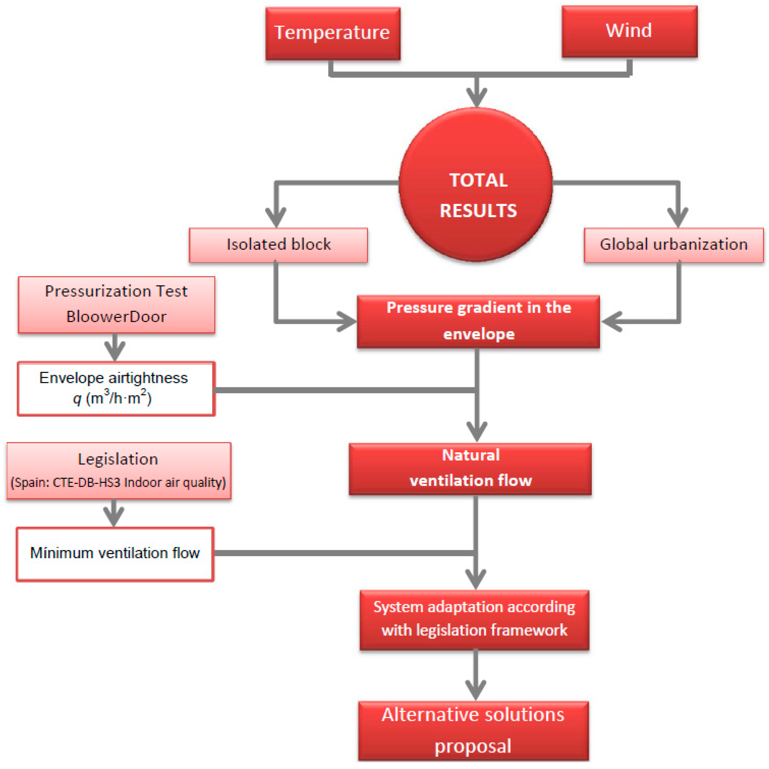
First, it is necessary to appropriately characterize the environment and how it influences natural ventilation conditions. The inlet of outdoor air into the building is based on pressure gradients resulting from the combined effect of two simultaneous processes: Free convection flow due to density differentials from the different temperatures on both sides of the enclosure and forced convection flow of natural origin due to wind (Figure 3) [17].
In simulations, it is common to use standardized reference environmental values. Nevertheless, we have selected specific values for the location in Laguna de Duero:
- Gravity for calculations (41°34′59″ N and 704 m a.s.l.) is = 9.80094 m/s2.
- Reference atmospheric pressure ( = 11.4 °C) is pa = 93,049 Pa.
- Density values ρext, ρo and ρint (from exterior, unconditioned, and interior spaces) [18] correspond to mean outdoor conditions for calculations (January ‘mean temperature’ Text = 3.0 °C/‘relative humidity’ RH = 85.3%, July Text = 20.5 °C/RH = 46.9%, and ‘annual mean temperature’ Text = 11.4 °C/RH = 65% [19]) in combination with other indoor comfort values for apartments (‘Dry-bulb temperature’ Tint = 23.0 °C/RH = 50%) and unconditioned spaces (winter To = 7.0 °C/RH = 65%, summer To = 21 °C/RH = 46%, and annual To = 13.7 °C/RH = 57%).
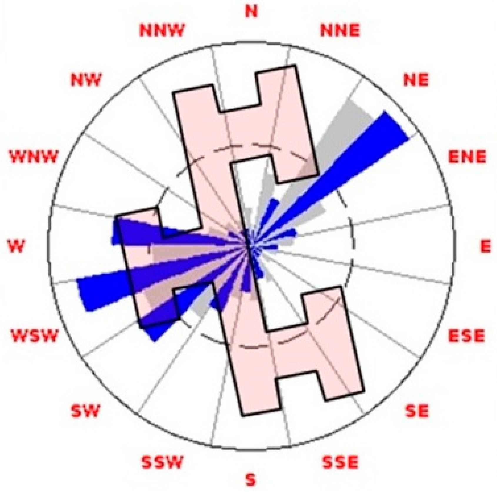
- The predominant wind pattern at the regional level is the so-called ‘Ábrego’, coming from the West-South West. To obtain a specific wind profile for the location, the national wind atlas [20] is used and includes a wind rose at a height of 80 m (Figure 4). The mean seasonal velocity at this height is 5.30 m/s in the winter, 4.55 m/s in the summer and 5.02 m/s annually. The predominant directions West-South West/South West and North East hit the blocks orthogonally.
3.1. Thermal Pressures
As a general rule, a temperature difference generates changes in air density that is translated into a pressure gradient, which causes air movement through enclosures. This phenomenon, which becomes particularly important in tall buildings [21], is called the stack effect. At a specified height, say zn, the gradient Δp is equal to zero, and this height is called the neutral line. In the winter (assuming that Tint > Text), Δp causes air to exit from the building above this height and enter into the building below this height [22,23]. The equation (Equation (1)) that expresses the pressure difference between the lower level and the higher level (H = top height of the vertical space) of a building is as follows:
In the Torrelago buildings, this process takes place through vertical integrated shafts within the building (elevators, stairwells, shafts, etc.), so the total gradient on the exterior enclosure can be calculated.
3.2. Wind Pressures
The geometric and roughness characteristics of the surrounding environment affect the pressure distribution on the envelope of buildings [24]. The physical phenomenon of wind in urban environments is numerically simulated by computational fluid dynamics (CFD) validated scale models.
This study simulates the wind behavior by applying certain boundary conditions (Table 1) that relate the physical properties of the model with the parameters of the air (internal friction, height of boundary layer, etc.). Physical and air parameters have been transposed from the experimental models in a wind tunnel in order to improve the representativeness of the evaluated cases. This minimizes the spread of results with respect to the reference models used for the validation and setting of the CFD model. These parameters cause wind movement in a free condition and therefore in the domain under study. To a greater or lesser extent, they allow that the moving air sticks on, detaches or flows, with more or less velocity and turbulence, along the delimiting surfaces of outdoor spaces.
The continuous variation of wind direction and velocity over short periods of time make it impossible to predict the exact air behavior unless a full transient simulation is carried out [25]. Any study of the air in urban environments requires taking various premises that significantly reduce the complexity of the physical model [26]. The envelopes of the building, with no roughness, are considered to have the same temperature as the air. The roughness and ground displacement heights provided by the experimental reference model are used. Theses premises avoid the dynamic conditioning on the velocity profile, which has been adapted to the climatic conditions of the site. Using steady wind inflow criteria reduces the complexity of the simulation. Wind simulation turns into a constant dependent on height over earth surface. The definition of the boundary conditions for wind profiles, such as velocity, turbulent kinetic energy and dissipation of turbulence (Equations (2)–(6)), is applied to the inlet of the simulated model [27].
Wind profiles participate in a non-uniform distribution of pressures on the surfaces of a building [29]. Turbulence phenomena in the built environment need to be considered in CFD [30]. Turbulence is responsible for the chaotic movement of the air, facilitating the formation of vortices and stagnation in protected areas to direct the action of simulated wind [31].
The computational model is defined by the boundaries enclosing the volume of air in the domain, being confined by the lateral walls of the experimental model.
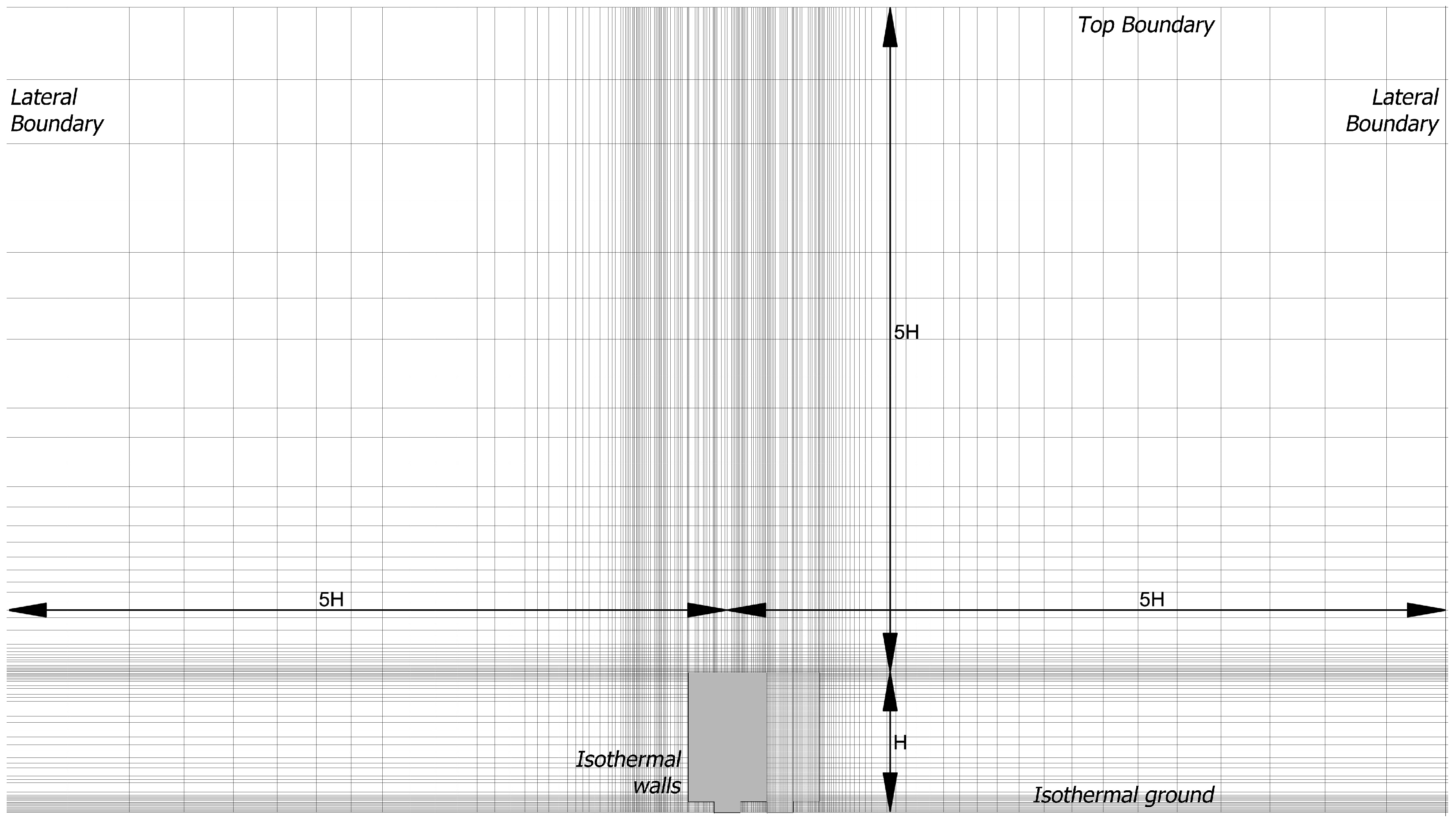
The domain of the simulation, made with software Ansys Fluent R15.0© (R15, ANSYS, Inc., Canonsburg, PA, USA), fulfils the dimensional requirements defined by the practice guideline for CFD [32], with a distance from the coordinate system origin of 8H (on the axis of symmetry of the model being calculated) to the walls (lateral and top), and 5H and 15H longitudinally upwind and downwind from the model, where H is the height of the building that serves as the obstacle. The analysis of the aerodynamic behavior of air next to the facades of the buildings requires the definition of a meshed model to ensure the right dynamic estimation due to the wall effect. For this ideal model domain, a three-dimensional hexahedral mesh is designed with a number of cells of ≈6 × 10⁶ for the isolated block and ≈3 × 10⁶ for urban development. For the individual block model, the cell size is progressively reduced in the vicinity of solid volumes (Figure 5), with a variation between contiguous cells of less than 10%. As a result, the smallest cell has a dimension of 0.006H (0.25 m), obtaining a y+ non-dimensional value of 14.45 which is smaller than the suggested one [27]. The boundary conditions used on the CFD model and adopted in the reference models for its validation determine the side and upper boundaries with similar conditions to the wind tunnel. On the other hand, the air inlet to the model is accomplished with velocity and turbulence profiles adapted to the site defined by the horizontal interior surface (ground). The (air) outlet occurs by defining the specific turbulence criteria of the case and limiting its ability to reproduce reflux.
A single mesh is used in the simularion of each building group. The representativeness of the study is achieved through a possible comparison of the results.
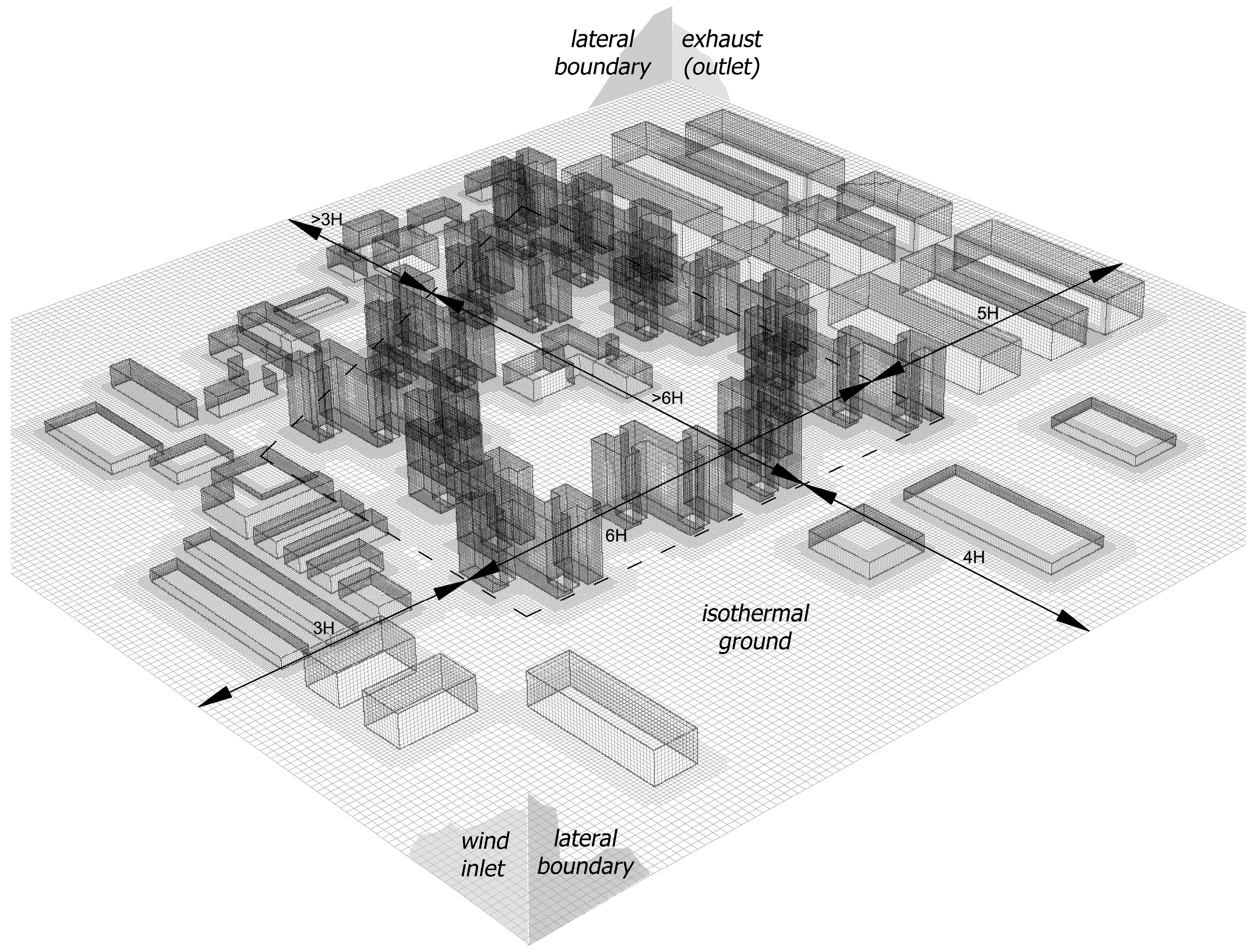
Due to the extension of the urban area, the lateral distance of 7H from the center of the analyzed site is exceeded. A mean of 3H from the external buildings on both sides of the model and the air inlet is reached. The upper limit is located at a distance of 6H from zero level. The air outlet is located at 5H fixing the no return of the circulated air condition. In the neighborhood-scale model, the mesh is uniform along the entire domain, becoming more refined in the vicinity of buildings. This type of solution, ideal for large fluid volumes, reduces the number of cells required to solve the functions in the vicinity of building enclosures [33]. The separation between nodes was fixed to make the nodes coincide with points where there are wind pressure readings on the façades, at a distance of 0.036H (1.5 m) (Figure 6).
The necessary validation of any numerical study must take into account the systematic differences between field tests, wind tunnel tests and computational simulations [34]. Field data in urban environments represent mean intervals that range from 10 to 30 min (larger intervals are not viable due to the continuous variation of meteorological conditions), causing poor reproducibility in the results. The CFD simulations respond adequately to steady conditions, which is why they are validated with reference data obtained in the wind tunnel using seasonal conditions.
The CFD validation procedure used in the research was conducted using the resources made available by the Environmental Wind Tunnel Laboratory (EWTL) in the Meteorological Institute at the University of Hamburg [35]. This organisation manages a compilation of datasets for the validation of microscale wind models clustered into the Compilation of Experimental Data for Validation of Microscale Dispersion Models (CEDVAL) project. The validation process developed by Padilla-Marcos et al. [33] consisted of the CFD recreation of case A1–4 (cubic building) available in the database. For this purpose, the boundary conditions and experimental wind parameters have been used and transposed as indicated in Table 1. Three models of turbulence (Skε (Standard-kε) [28]; RNG (Re-Normalization Group) [36] and; Realizable [37]) were used to refine the simulated behavior in the experimental results. Sequential simulations were carried out with two options for the evaluation of the wall effect (Standard Wall Functions (SWF) and Enhanced Wall Treatment (EWT)) under a criterion of SIMPLE resolution and spatial discretization based on a steady Green-Gauss Node-Based analysis [27]. The Realizable turbulence model (Realizable EWT) has been the most accurate at evaluating together the net velocity (Velocity magnitude) and the predominant wind direction (X Velocity).
The design of the hexahedral mesh evaluates the wall effect on the viscous sublayer by its refinement in the proximity of the buildings. The suitability of the mesh has been verified for the analized spatial discretization criteria by fixing measurement nodes at the points of interest (local mean deviation), reaching (mesh and experimental configuration criteria together) a mean deviation of less than 4%. That accuracy, obtained through point-to-point testing of the computer’s calculation precision, was estimated for all sampling points (Table 2), with a higher deviation in the points close to a single obstacle compared with the entire sample, but always less than the maximum and commonly accepted deviation of 5%. Similarly, the greatest concentration of point mean deviations occurs in the lower layers of the model (<0.1H) and on surfaces in contact with the solid volume due to the high turbulent energy that is generated.
Case B1–2 of the CEDVAL project extends the reference case to an urban model of ring-shaped buildings. The suitability of the validated configuration for the cubic building was verified in the urban environment. Testing a full urban model, better precision was obtained with the RNG-SWF and Realizable EWT models where more than 40% of the sampled points differ by less than 10% with the experimental results (Table 3 and Table 4).
A deviation of less than 4% was achieved for axial velocities (X Velocity). Mean precision for the wind velocity magnitude was above 95% (Table 4). This level of precision was obtained in simulations under the RNG viscosity model with application of SWFs compared with the EWT method [38]. Even more precise validation results were obtained under the ‘Realizable’ numerical model, which required greater computational cost. Validation results had shown that lower layers of air, which are placed adjacent to the ground surface, differ from those obtained in the EWTL tests. This is due to the generated wall shear stress and the measuring difficulty within the tests. Nevertheless, the results obtained adjacent to and above the buildings in the CFD replicate the measured data well.
According to the assumptions discussed in the validation process, two simultaneous situations are simulated. Both situations, isolated block and whole district, are simulated to approximate the numerical value of the wind pressure on the envelope of buildings in the simulated urban environment. The accuracy of the results of the scaled experiences under RANS turbulence models with Enhanced Wall Treatment (EWT) satisfy the requirements of representativeness for the analysis of the aerodynamic behavior near façades [39]. The results are obtained with a convergence criterion lower than 10−8 for which more than 25,000 iterations are required for each case. The quality of the simulation has been evaluated by means of successive domains of control (surrounding the buildings), in which the flow balance between the air inlets and outlets was verified. Special attention was paid to the equilibrium in the computational domain, resulting in a convergence lower than 3 × 10⁻⁵.
3.3. Combined Thermal and Wind Effects
The superposition of pressures resulting from temperature and wind effects allows for calculation of their effects on the surface of each of the enclosures that envelope the apartments [40] (Table 4). The resultant effects represent different cases throughout the year, with alternating seasonal pressure and suction forces on the higher and lower floors.
3.4. Permeability of Enclosures
Pressure tests in apartments can determine the permeability of the enclosure with the ability to differentiate between the values for blind spots and openings. The test, carried out according to European Norm EN 13829 [41], and commonly called the Blower Door Test, creates a pressure differential inside the tested apartment with respect to outdoors, measuring the air flow that circulates through a fan. In an initial phase, the test is performed using method B of the rule (test on the building enclosure), progressively sealing the more significant infiltration points (framed openings, shutter boxes) to establish the effects they have on enclosure permeability. Subsequently, method A is applied (test for a building being used) to verify the state of the shared ventilation shunts.
The infiltration flow rate obtained from the test is measured as a function of the pressure gradient through the building enclosure, adopting a power law (Equation (7)):
where CL is the power law coefficient (m3/h·Pan), ∆p is the pressure difference (Pa), and n is the power law exponent. The coefficient CL depends on the filtration area. The exponent n depends on the resistance of the filtration openings to the passage of air, and it represents the three-dimensional geometry of the filtration openings (height, width, and depth) and the physics of air transport [42,43]. This function allows for calculation of the infiltration flow rate equivalent to the desired pressure gradient, which enables quantification of the air that penetrates each of the wall surfaces.
The construction characteristics of the blocks leads to the assumption that infiltrations calculated this way occur mostly through the outer building enclosure:
- Apartments are separated from other apartments on the same floor using medium-heavy enclosures, without sharing common elements that interrupt that continuity.
- The test uses the access door to the apartment as a place to locate the ventilator, which translates into the virtual sealing of this weak point separating the apartment from common areas of the building.
- Plumbing is installed inside of the apartment without going through the enclosure. Vertical lines use independent shafts.
- Sealing all framed openings and identified infiltration points resulted in tests with practically no rate of infiltration through the rest of the enclosure.
3.5. Natural Ventilation Flow Rate
Based on the data shown, it is possible to quantify the natural ventilation flow rate of each apartment located in an isolated block through a process that simultaneously analyzes the different elements of the enclosure exposed to pressure gradients. The procedure is based on the EN 13465 [44], which follows the guidelines in classical natural ventilation theory (Figure 7).
This method is based on a unique zone model representing each evaluated dwelling as an individual zone with a global pressure value, obtained alternatively according to the flow balance equation between the inlet and outlet air flows. The ventilation air flow (opening of windows by the users) is not considered in the calculation, since it is considered as an additional and voluntary air flow.
In this sense, the inlet air flow is equal to the system flow (qv ext = qv syst), obtained according to the balance equation between the leakage qv leak air volume through the opaque areas of the envelope, transparent areas of the envelope, and the draught in the vertical ducts qv vent (Equation (8)):
This equation has to be solved for the unknown internal pressure pint using the equations (Equations (9)–(13)):
where lpi is the infiltration i related to the global infiltration through the building envelope, and V is the volume of the building.
The pressure gradient ∆pint/ext is defined based on the temperature gradient (Tint − Text) and the pressure gradient at the duct outlet in the roof pk.
The formulated systems of equations require the use of the Engineering Equation Solver EES (version V8.400, F-Chart Software, University of Wisconsin-Madison, Madison, WI, USA) calculation software to determine the indoor pressure and the system flow rate qv syst (which is equivalent to the natural ventilation flow).
4. Results
The results obtained by the described methodology are presented independently according to its definition by thermal or wind conditions [45]. Afterwards, the repercussions that they have together on conditions to produce the desired natural ventilation will be analyzed.
4.1. Thermal Pressures
The entire building has been analyzed throughout its height evaluating the pressure gradient formed by the thermal difference at different heights of the building. Hypothetical conduits in its interior (shafts, elevator, chimneys and stairwells) that lead to the formation of the passive stack effect have been considered. The pressure gradient conditions the air's ability to access or exit the building through its envelope (Figure 8).
In winter conditions, the greater pressure gradient is considered, a stack effect produced with a thermal difference of 16 °C, when the inner air has more thermal energy than the outside air. In summer conditions, when the thermal difference is reduced to 2 °C, the stack effect does not reverse since the inner air still has more energy than the outside air. Due to this circumstance, the pressure gradient is considerably reduced.
The facade in the lower part of the building is subjected to static pressure due to the effect of the density difference of the air contained in the building which fosters the entrance of outside air. On the contrary, the upper floors are subject to static suction caused by the accumulation of air with a lower density. That is to say, the hot air inside the building presses the inner face of the envelopes causing an evasive air phenomenon. The direct entrance of air for the ventilation of the dwellings located in the upper floors of the building is hindered.
The numerical results show that the neutral line of pressures occurs at an approximate height at the middle of the elevation (Central level—6th). This phenomenon occurs in the three evaluated climatic conditions: winter, summer and annual average (January, July and Annual average, respectively).
4.2. Wind Pressures
The positive or negative pressure that the wind exerts on the buildings defines the field of study. It qualifies the process of natural indoor air renovation. This conditioning is caused by the dynamic action of the wind that pressurizes or sucks the envelopes causing the entrance of air in a controlled or uncontrolled way. Checked entrance of air would respond to the building design (holes, grids, courtyards, shunts, etc.) in order to foster an indoor air renovation. The uncontrolled entrance of the air is largely caused by construction imperfections (cracks, joinery, gaps, etc.) that compromise the design of the ventilation system.
4.2.1. Results in an Isolated Block
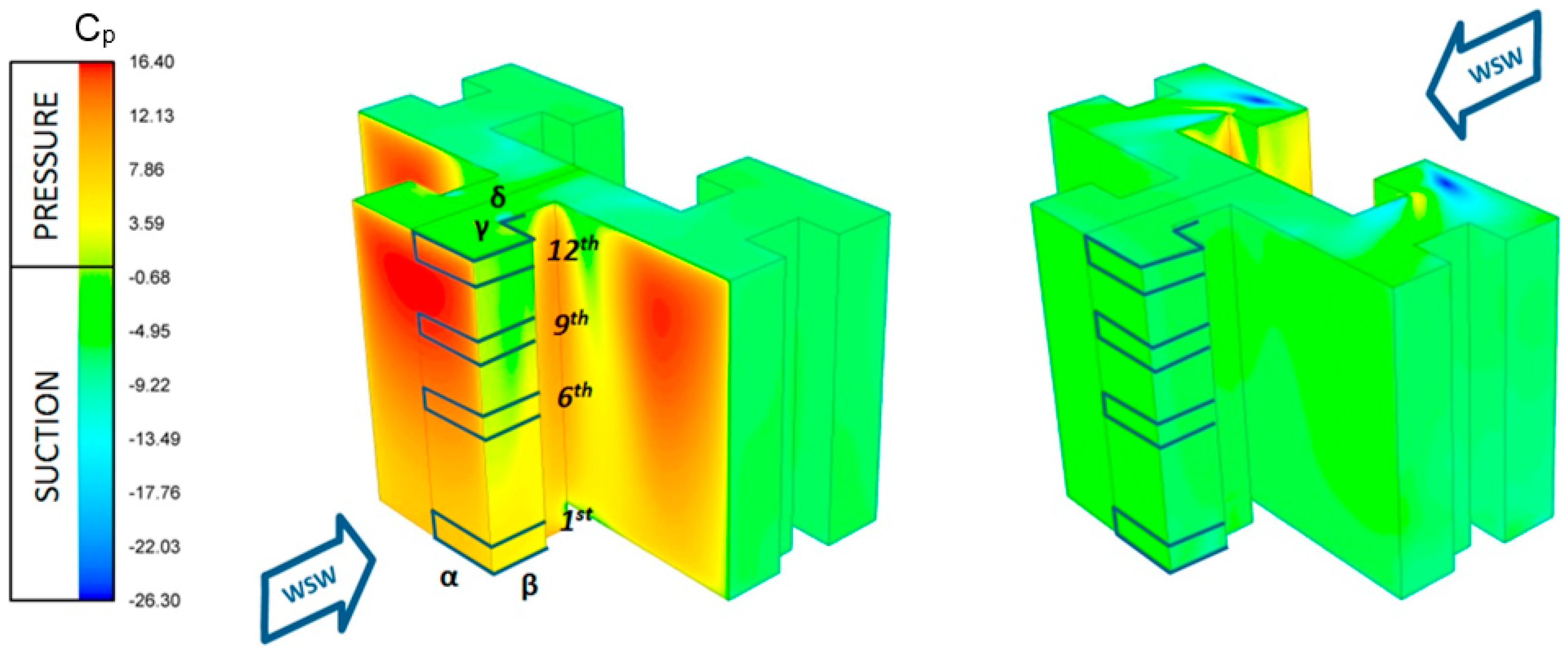
Ten variations were studied for the isolated building, with different orientations, seasonalities, exposures to wind and groupings with other H-shaped blocks. The obtained CFD simulation provides a large amount of model flow data: velocity distributions, static and dynamic pressures, particle trajectory, age of the air, and other parameters. For example, the wind pressure coefficient for the enclosures allows differentiation between areas subjected to pressure and suction effects as a result of wind action and then obtaining their Pascal values [46,47]. Generally speaking, we consider pressure gradients between −0.03 and 11.64 Pa for windward enclosures and between −2.85 and −5.69 Pa for leeward (Table 4). A detailed analysis requires characterizing these pressures at different elevations on the building corresponding with the variable wind velocity profile. The values obtained for different enclosures for each of the apartments establishes the total pressure gradient resulting from wind action. This study focused on the wind coming from the WSW and NE directions, which are predominant throughout the year, converting the wind action to orthogonal pressure on the façades. In terms of the heights considered, pressure values were calculated for the lower (1st), central (6th), reference (9th) and upper (12th) levels. Finally, the different orientations of the parameters for a single apartment are characterized using the Greek letters α, β, γ and δ. (Figure 9).
4.2.2. Urban Model Results
The simulation at the district level identifies the features that intercept the free flow of the wind, altering the air displacement in the downwind regions. In that respect, we must highlight that the influence of corridors, open areas and building walls always requires a specific study that quantifies the effects of natural ventilation on each building compared to behavior when they are isolated [48,49,50,51].
This study used the mean annual values for wind acting from the predominant WSW and NE directions (Figure 10). The results confirm that the most-exposed buildings can be similar to isolated blocks. In turn, they simultaneously act as screens for those located downwind, mitigating the wind pressures on their enclosures by an order of 70%–90%. This result implies an analogous reduction of the available natural ventilation flow rate.
As previously shown, the most exposed buildings are those able to have a greater flow rate of natural ventilation. The buildings that are protected from the dynamic action of the wind (shield effect) will be affected in a greater extent by the convective phenomena due to the thermal difference between the interior and the exterior.
4.3. Combined Results
The superposition of pressures resulting from temperature and wind effects allows calculating their effects on the surface of each of the enclosures that enclose the apartments (Table 5).
Pressurization testing has given some information about the initial conditions of the building and the impact of spontaneous interventions by owners as well. It occurs particularly with regard to the substitution of framed openings and the sealing of shared ventilation shunts (Table 6).
In this manner, the natural flow rate for the ventilation of an isolated block is simulated based on different parameters of the apartments. They are affected by their height in the building, the mean exposure to predominant wind directions and the construction configuration in accordance with the original project (Table 7).
5. Discussion
The flows obtained vary, as it could be supposed, depending on the floor in which the dwelling is located and the climate conditions (Figure 11). Once the available flows are calculated, it is possible to compare these values with the minimum requirements established in national regulations (in Spain, the Building Code CTE DB-HS3, Indoor Air Quality [52]). These values are only valid for the buildings with the most exposure given that there are others in the urban development with reduced flow rates by as much as 90% due to the screen effect, as described previously.
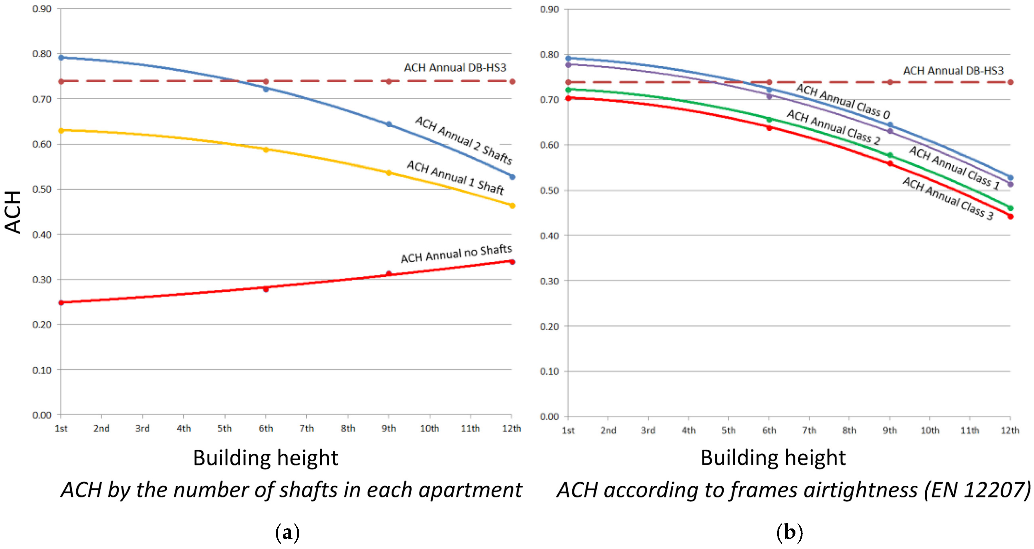
In some cases the users have introduced modifications to the original project. When modifying the terms of the balance equation (Equation (8)), it is possible to identify the influence of these singular parameters (Figure 12):
- The refurbishment of bathrooms and kitchens has obstructed some or in some cases all vertical ducts for ventilation. The term allows simulation of these changes, calculating the influence of the existence of these ducts in the available natural ventilation flow.
- The replacement of windows affects two different parameters: transmittance, and air permeability. When referred to natural ventilation, the flows are drastically reduced in new windows, which may provoke the need to install additional ventilation openings.
6. Conclusions
The combined evaluation of wind and convective action of the air on natural ventilation allows for the analysis of the impact of the used criteria.
The considered methodology combines different tools to justifiably estimate natural ventilation flows. The need arises when simplified methods (ASHRAE [53], Florida Solar Energy Center [54], Givoni [55], CSTB [56], Ernest [57], etc.) are found to be minimally applicable to complex simulations, since they are based on very basic assumptions: uniform wind pressure, obstacle simplification, etc.
This methodology is extendable to other study cases using available tools for researchers:
- (1)
- Official climatic data, stabilized in time, are used.
- (2)
- CFD configuration validated through wind tunnel experimentation data, making them secure for late wind simulation on urban developments in stationary conditions.
- (3)
- The combination of wind and thermal pressures, being these dependent on temperature conditions, provide the total gradient over each of the envelope surfaces, according to its height and orientation.
- (4)
- Envelope permeability experimentally determined on site with pressurization tests.
- (5)
- Consequently, pressure equilibrium equations consider all the possible factors, solving for the resultant interior pressure and the available flow on the system.
- (6)
- Finally, by varying singular parameters on the equation, it is also possible to quantify their influence on the final considered value.
The application of this methodology enables the correct characterisation of natural ventilation availability on existing buildings. It is concluded that, under winter conditions, the ventilation requirements set by Spanish regulations are met for the 4BR case when the apartment heights are lower than the 9th floor. Under summer conditions, the requirements are not met at any height. In the case of the annual average, they are only met in the lower third of the 4BR case. The 3BR case does not meet requirements at any height.
Acknowledgments
The research leading to these results has been carried out under the CITyFiED project, which has received funding from the European Union’s Seventh Framework Programme for research, technological development and demonstration activities under the Grant Agreement number 609129.
Author Contributions
Alberto Meiss and Miguel A. Padilla-Marcos, designed and performed the experiments; Alberto Meiss, Jesús Feijó-Muñoz and Jesús Feijó-Muñoz contributed reagents/materials/analysis tools; Alberto Meiss and Miguel A. Padilla-Marcos analyzed the data and wrote the paper.
Conflicts of Interest
The authors declare no conflict of interest.
References
- Etheridge, D. Natural Ventilation of Buildings; John Wiley & Sons Ltd.: Chichester, UK, 2012. [Google Scholar]
- Chiu, Y.-H. Development of Unsteady Design Procedures of Natural Ventilation Stacks. Ph.D. Thesis, University of Nottingham, Nottingham, UK, 2004. [Google Scholar]
- Turner, W.J.N.; Awbi, H.B. Experimental investigation into the thermal performance of a residential hybrid ventilation system. Appl. Therm. Eng. 2015, 77, 142–152. [Google Scholar] [CrossRef]
- Tong, Z.; Chen, Y.; Malkawi, A.; Liu, Z.; Freeman, R.B. Energy saving potential of natural ventilation in China: The impact of ambient air pollution. Appl. Energy 2016, 179, 660–668. [Google Scholar] [CrossRef]
- Majcen, D.; Itard, L.; Visscher, H. Actual heating energy savings in thermally renovated Dutch dwellings. Energy Policy 2016, 97, 82–92. [Google Scholar] [CrossRef]
- Pisello, A.L.; Castaldo, V.L.; Taylor, J.E.; Cotana, F. The impact of natural ventilation on building energy requirement at inter-building scale. Energy Build. 2016, 127, 870–883. [Google Scholar] [CrossRef]
- Sorgato, M.J.; Melo, A.P.; Lamberts, R. The effect of window opening ventilation control on residential building energy consumption. Energy Build. 2016, 133, 1–13. [Google Scholar] [CrossRef]
- Kinnane, O.; Sinnott, D.; Turner, W.J.N. Evaluation of passive ventilation provision in domestic housing retrofit. Build. Environ. 2016, 106, 205–218. [Google Scholar] [CrossRef]
- Huang, K.-T.; Hwang, R.-L. Parametric study on energy and thermal performance of school buildings with natural ventilation, hybrid ventilation and air conditioning. Indoor Built Environ. 2016, 25, 1148–1162. [Google Scholar] [CrossRef]
- Pabiou, H.; Salort, J.; Ménézo, C.; Chillà, F. Natural cross-ventilation of buildings, an experimental study. Energy Procedia 2015, 78, 2911–2916. [Google Scholar] [CrossRef]
- Budiakova, M. Architectural design of university schoolrooms with the link to ventilation. Proceedings of World Multidisciplinary Civil Engineering-Architecture-Urban Planning Symposium 2016, WMCAUS 2016, Prague, Czech Republic, 13–17 June 2016. [Google Scholar]
- Shen, C.; Li, X. Thermal performance of double skin facade with built-in pipes utilizing evaporative cooling water in cooling season. Sol. Energy 2016, 137, 55–65. [Google Scholar] [CrossRef]
- Sim, J.K.; Cho, Y.-H. Portable sweat rate sensors integrated with air ventilation actuators. Sens. Actuators B Chem. 2016, 234, 176–183. [Google Scholar] [CrossRef]
- Nejat, P.; Calautit, J.K.; Majid, M.Z.A.; Hughes, B.R.; Jomehzadeh, F. Anti-short-circuit device: A new solution for short-circuiting in windcatcher and improvement of natural ventilation performance. Build. Environ. 2016, 105, 24–39. [Google Scholar] [CrossRef]
- CITyFIED Project. Available online: http://es.cityfied.eu/ (accessed on 21 March 2017).
- Meiss, A.; Feijó-Muñoz, J.; Padilla-Marcos, M.A.; Vasallo, A.; Méndez, E. D2.5: Methodology for Natural Processes Based on the Ventilation Systems Evaluation and Implementation; CITyFIED Project; Fundación CARTIF: Valladolid, Spain, 2015. [Google Scholar]
- Li, J.; Ward, I.C. Developing computational fluid dynamics conditions for urban natural ventilation study. In Proceedings of the IBPSA Proceedings: Building Simulation, Beijing, China, 3–6 September 2007. [Google Scholar]
- Davis, R.S. Equation for the determination of the density of moist air (1981/91). Metrologia 1992, 29, 67–70. [Google Scholar] [CrossRef]
- Instituto para la Diversificación y Ahorro de la Energía. Guía técnica de Condiciones Climáticas Exteriores de Proyecto; IDAE: Madrid, Spain, 2010. (In Spanish) [Google Scholar]
- Instituto para la Diversificación y Ahorro de la Energía Atlas eólico de España. Atlas eólico de España. Available online: http://atlaseolico.idae.es/meteosim/ (accessed on 21 March 2017). (In Spanish).
- Yang, W.; Gao, N. The Transport of gaseous pollutants due to stack effect in high-rise residential buildings. Int. J. Vent. 2015, 14, 191–208. [Google Scholar] [CrossRef]
- Jo, J.; Lim, J.; Song, S.; Yeo, M.; Kim, K. Characteristics of pressure distribution and solution to the problems caused by stack effect in high-rise residential buildings. Build. Environ. 2007, 42, 263–277. [Google Scholar] [CrossRef]
- Khoukhi, M.; Al-Maqbali, A. Stack pressure and airflow movement in high and medium rise buildings. Energy Procedia 2011, 6, 422–431. [Google Scholar] [CrossRef]
- Hussain, M.; Lee, B.M. An Investigation of Wind Forces on Three Dimensional Roughness Elements in a Simulated Atmospheric Boundary Layer; Report BS 55; Department of Building Science, University of Sheffield: Sheffield, UK, 1980. [Google Scholar]
- Sutton, O.G. Atmospheric turbulence. Q. J. R. Meteorol. Soc. 1949, 76, 108. [Google Scholar]
- Amorim, J.H.; Rodrigues, V.; Tavares, R.; Valente, J.; Borrego, C. CFD modelling of the aerodynamic effect of trees on urban air pollution dispersion. Sci. Total Environ. 2013, 461, 541–551. [Google Scholar] [CrossRef] [PubMed]
- Fluent Inc. FLUENT 6.1 User’s Guide; Fluent Inc.: Lebanon, NH, USA, 2003. [Google Scholar]
- Launder, B.E.; Spalding, D.B. The numerical computation of turbulent flows. Comput. Methods Appl. Mech. Eng. 1974, 3, 269–289. [Google Scholar] [CrossRef]
- Sutton, O.G. The logarithmic law of wind structure near the ground. Q. J. R. Meteorol. Soc. 1936, 62, 124–127. [Google Scholar] [CrossRef]
- Richards, P.J.; Hoxey, R.P. Appropriate boundary conditions for computational wind engineering models using the k-ε turbulence model. J. Wind Eng. Ind. Aerodyn. 1993, 46, 145–153. [Google Scholar] [CrossRef]
- Hotchkiss, R.S.; Harlow, F.H. Air Pollution Transport in Street Canyons; United States Environmental Protection Agency Report EPA-R4-73-029; Environmental Protection Agency: Washington, DC, USA, 1973.
- Franke, J.; Hellsten, A.; Schlünzen, H.; Carissimo, B. Best Practice Guideline for the CFD Simulation of Flows in the Urban Environment; COST Action 732: Hamburg, Germany, 2007. [Google Scholar]
- Padilla-Marcos, M.A.; Feijó-Muñoz, J.; Meiss, A. Wind velocity effects on the quality and efficiency of ventilation in the modelling of outdoor spaces. Case studies. Build. Serv. Eng. Res. Technol 2016, 37, 33–50. [Google Scholar] [CrossRef]
- Sharples, S.; Bensalem, R. Airflow in courtyard and atrium buildings in the urban environment: A wind tunnel study. Sol. Energy 2001, 70, 237–244. [Google Scholar] [CrossRef]
- Leitl, B.; Schatzmann, M. Validation Data for Microscale Dispersion Modelling; EUROTRAC Newsletter 22; EUROTRAC: Göteborg, Sweden, 2000. [Google Scholar]
- Yakhot, V.; Orszag, S.A.; Thangam, S.; Gatski, T.B.; Speziale, C.G. Development of turbulence models for shear flows by a double expansion technique. Phys. Fluids 1992, 4, 1510–1520. [Google Scholar] [CrossRef]
- Shih, T.H.; Liou, W.W.; Shabbir, A.; Yang, Z.; Zhu, J. A New K-epsilon Eddy Viscosity Model for High Reynolds Number Turbulent Flows: Model Development and Validation. Comput. Fluids 1995, 24, 227–238. [Google Scholar] [CrossRef]
- Kim, J.J.; Baik, J.J. A numerical study of the effects of ambient wind direction on flow and dispersion in urban street canyons using the RNG k-epsilon turbulence model. Atmos. Environ. 2004, 38, 3039–3048. [Google Scholar] [CrossRef]
- Hertwig, D.; Efthimiou, G.C.; Bartzis, J.G.; Leitl, B. CFD-RANS model validation of turbulent flow in a semi-idealized urban canopy. J. Wind Eng. Ind. Aerodyn. 2012, 111, 61–72. [Google Scholar] [CrossRef]
- Micallef, D.; Buhagiar, V.; Borg, S.P. Cross-ventilation of a room in a courtyard building. Energy Build. 2016, 133, 658–669. [Google Scholar] [CrossRef]
- Comité Européen de Normalisation. EN 13829 Thermal Performance of Buildings. Determination of Air PERmeability of Buildings. Fan Pressurization Method; ISO 9972:1996, Modified; Comité Européen de Normalisation: Brussels, Belgium, 2002. [Google Scholar]
- Sherman, M.H.; Chan, W.R. Building air tightness: Research and practice. In Building Ventilation: The State of the Art; Santamouris, M., Wouters, P., Eds.; Routledge: Oxford, UK, 2006; pp. 137–162. [Google Scholar]
- Robertson, J.A. Effect of Building Airtightness and Fan Size on the Performance of Mechanical Ventilation Systems in New U.S. Houses: A Critique of ASHRAE Standard 62.2-2003. Master’s Thesis, University of California, Berkeley, CA, USA, 2004. [Google Scholar]
- Comité Européen de Normalisation. EN 13465:2004 Calculation Methods to Obtain Air Flow Rate in Apartments; Comité Européen de Normalisation: Brussels, Belgium, 2004. [Google Scholar]
- Meiss, A.; Feijo-Muñoz, J.; Padilla-Marcos, M.A. Evaluación, diseño y propuestas de sistemas de ventilación en la rehabilitación de edificios residenciales españoles. Estudio de caso. Inf. Constr. 2016, 68, e148. (In Spanish) [Google Scholar] [CrossRef]
- Gavanski, E.; Uematsu, Y. Local wind pressures acting on walls of low-rise buildings and comparisons to the Japanese and US wind loading provisions. J. Wind Eng. Ind. Aerodyn. 2014, 132, 77–91. [Google Scholar] [CrossRef]
- Rosa, L.; Tomasini, G.; Zasso, A.; Aly, A.M. Wind-induced dynamics and loads in a prismatic slender building: A modal approach based on unsteady pressure measurements. J. Wind Eng. Ind. Aerodyn. 2012, 107, 118–130. [Google Scholar] [CrossRef]
- Moonen, P.; Dorer, V.; Carmeliet, J. Effect of flow unsteadiness on the mean wind flow pattern in an idealized urban environment. J. Wind Eng. Ind. Aerodyn. 2012, 104, 389–396. [Google Scholar] [CrossRef]
- Blocken, B.; Carmellet, J.; Stathopoulos, T. CFD evaluation of wind speed conditions in passages between parallel buildings—Effect of wall-function roughness modifications for the atmospheric boundary layer flow. J. Wind Eng. Ind. Aerodyn. 2007, 95, 941–962. [Google Scholar] [CrossRef]
- Moonen, P.; Dorer, V.; Carmeliet, J. Evaluation of the ventilation potential of courtyards and urban street canyons using RANS and LES. J. Wind Eng. Ind. Aerodyn. 2011, 99, 414–423. [Google Scholar] [CrossRef]
- Tong, Z.; Chen, Y.; Malkawi, A. Defining the Influence Region in neighborhood-scale CFD simulations for natural ventilation design. Appl. Energy 2016, 182, 625–633. [Google Scholar] [CrossRef]
- Ministerio de Fomento. Gobierno de España. Código Técnico de la Edificación. Calidad del aire interior (DB HS-3). RD314/2006. Available online: http://www.codigotecnico.org/images/stories/pdf/salubridad/DBHS.pdf (accessed on 21 March 2017). (In Spanish).
- ASHRAE. Fundamental Handbook, Ch.26.10, Natural Ventilation; American Society of Heating, Refrigeration and Air Conditioning Engineers (ASHRAE): Atlanta, GA, USA, 2001. [Google Scholar]
- Chandra, S.; Farinley, P.W.; Houston, M.M. A handbook for Designing Ventilated Buildings. Florida Solar Energy Centre, Final Report; Florida Solar Energy Centre: Cape Canaveral, FL, USA, 1983. [Google Scholar]
- Givoni, B. Man, Climate and Architecture, 2nd ed.; Elsevier: New York, NY, USA, 1976. [Google Scholar]
- Centre Scientifique et Tecnique du Batiment. Guide sur la climatisasione naturelle de l’habitat et climat tropical humide—Methodologie de prise en compte des parameters climatiques dans l’habitat et conseil pratiques, Tome 1; CSTB: Marne-la-Vallée, France, 1992. (In French) [Google Scholar]
- Ernest, D.R. Predicting Wind-Induced Air Motion, Occupant Comfort and Cooling Loads in Naturally Ventilated Buildings. Ph.D. Thesis, University of California, Berkeley, CA, USA, 1991. [Google Scholar]
Figure 1.
(a) View of the Torrelago district from the lake; (b) Urban environment classification; (c) Aerial view; and (d) Area being simulated [16].
Figure 1.
(a) View of the Torrelago district from the lake; (b) Urban environment classification; (c) Aerial view; and (d) Area being simulated [16].
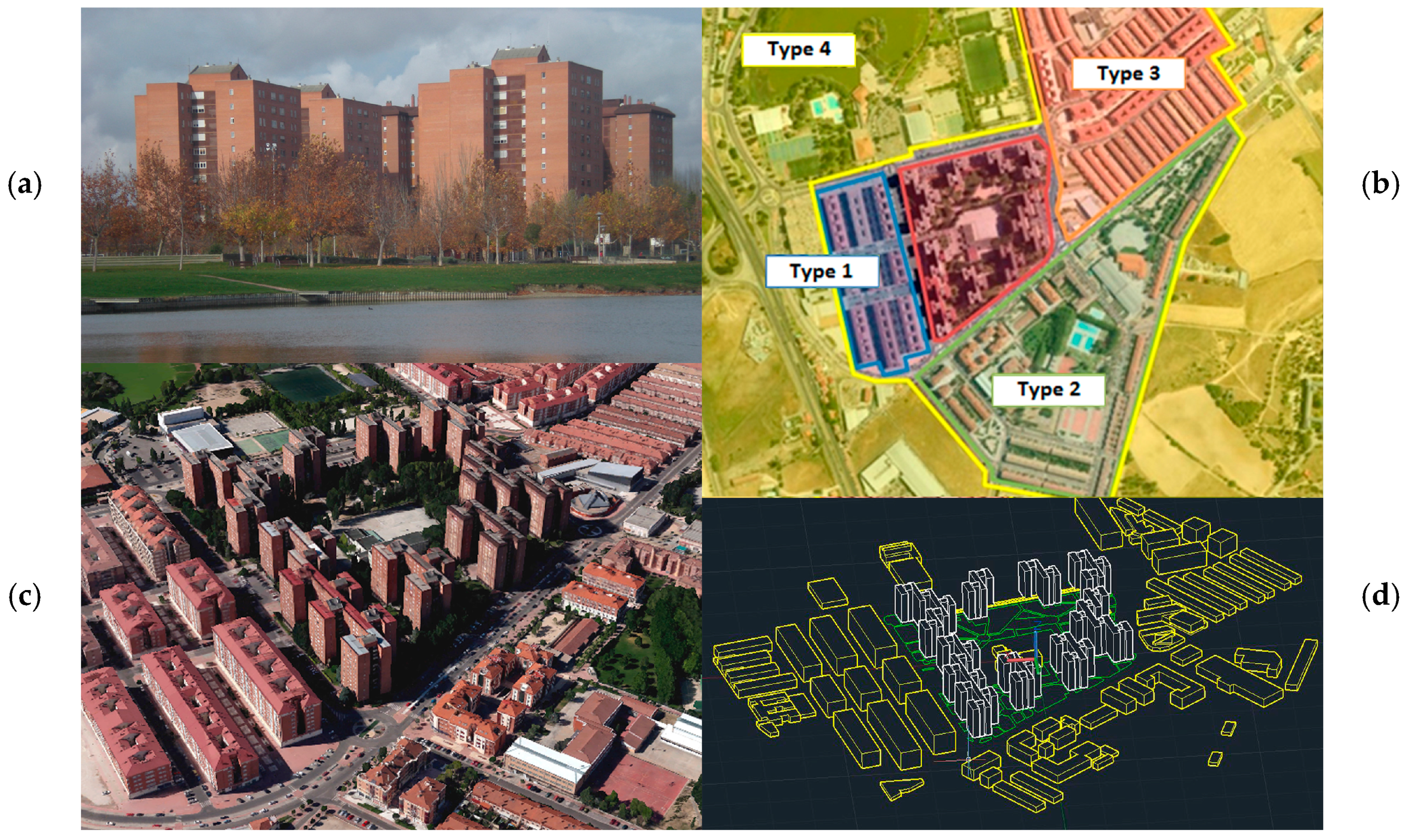
Figure 2.
(a) Type B Block with 3- and 4-bedroom apartments; (b) Urban District Typology.
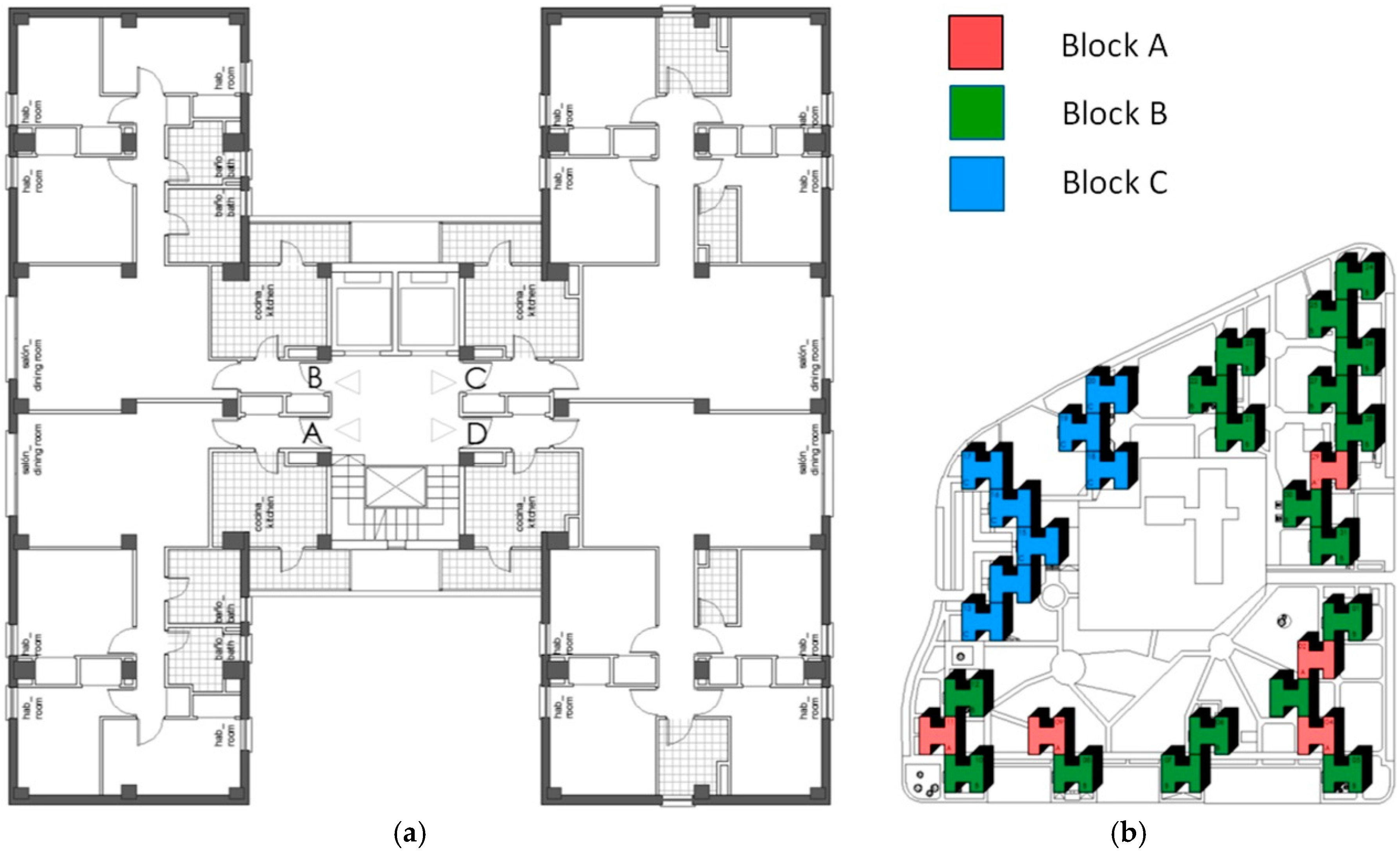
Figure 3.
Flow chart to obtain pressure gradients.

Figure 4.
Wind rose respect to blocks. W: West; WSW: West-South West; SW: South West; SSW: South-South West; S: South; SSE: South-South East; SE: South East; ESE: East-South East; E: East; ENE: East-North East; NE: North East; NNE: North-North East; N: North; NNW: North- North West; NW: North West; WNW: West-North West.

Figure 5.
Crosswise section of the computational fluid dynamics (CFD) meshed model.

Figure 6.
Three-dimensional view of the meshed CFD urban model.

Figure 7.
Procedure to quantify the natural ventilation flow rate of each dwelling.

Figure 8.
Pressure gradient resulting from temperature differences.
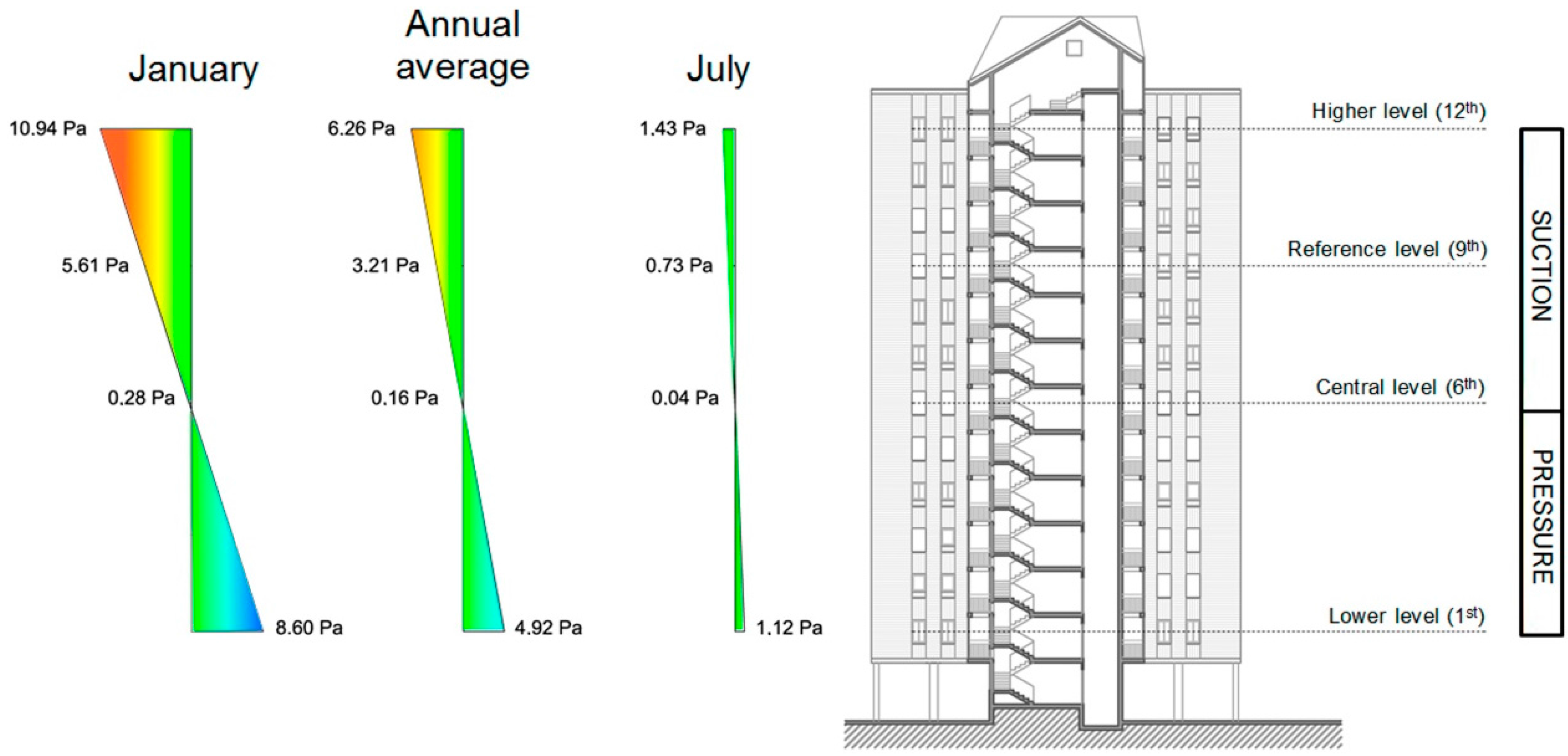
Figure 9.
Wind pressure coefficient (annual mean) for representative building enclosures.

Figure 10.
Wind pressure coefficient due to distribution from the WSW at district level.
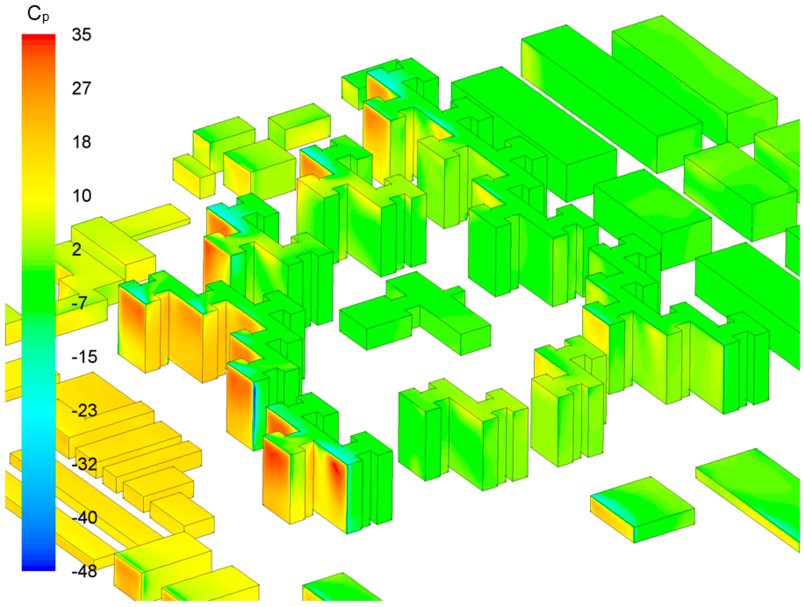
Figure 11.
Influence of the different apartment’s heights and climate conditions. ACH: Air change rate; BR: Number of bedroom.
Figure 11.
Influence of the different apartment’s heights and climate conditions. ACH: Air change rate; BR: Number of bedroom.
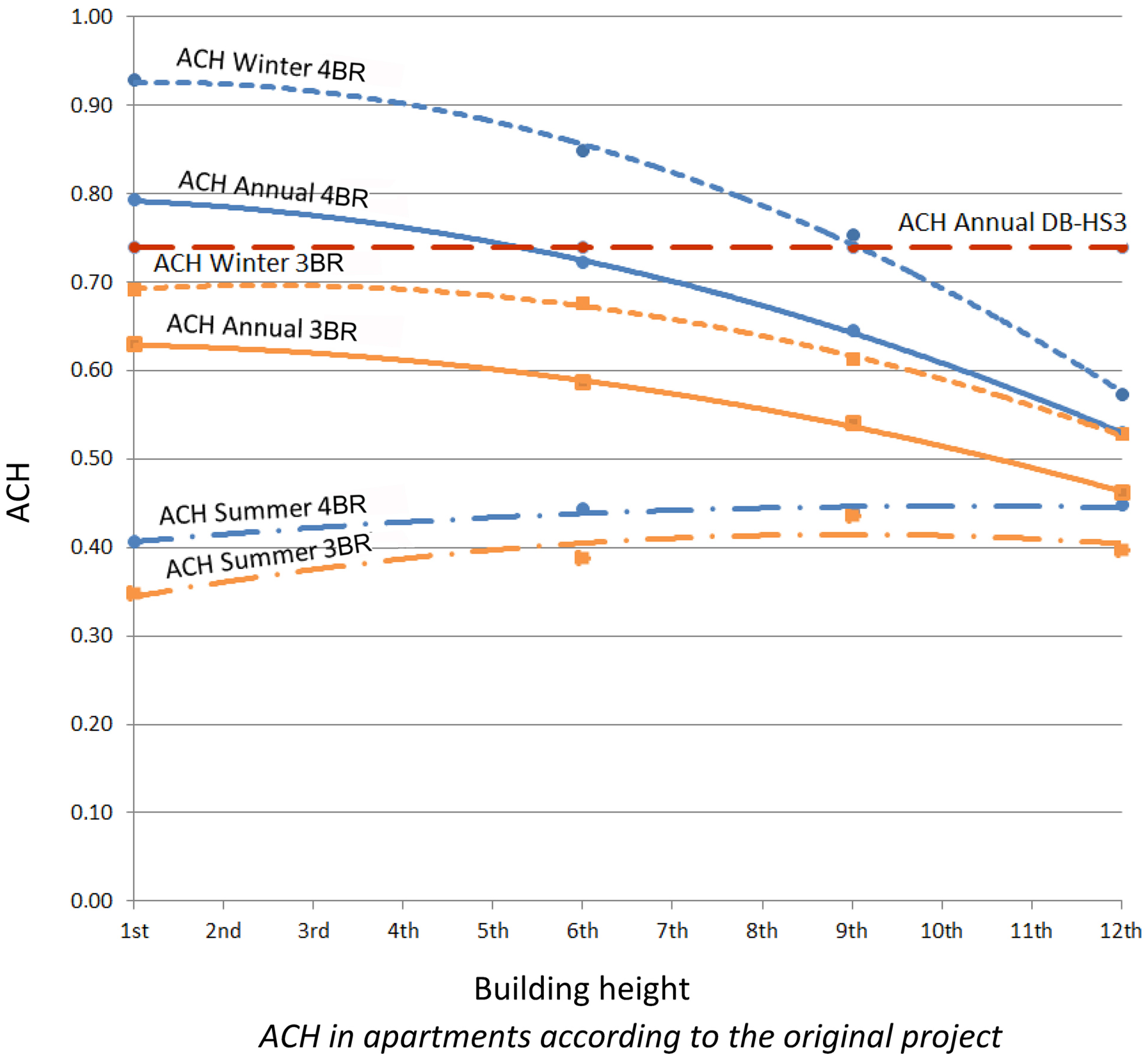
Figure 12.
Influence of the modifications to the original project. (a) Air change rate by the number of shafts; (b) Air change rate by airtightness of frames.
Figure 12.
Influence of the modifications to the original project. (a) Air change rate by the number of shafts; (b) Air change rate by airtightness of frames.


Table 1.
Boundary conditions applied in the numerical model.
| Air Characteristics (Fluid) | Inlet (Boundary Conditions) | ||||
| air density | 1.204 | kg/m³ | reference wind velocity | 3.000 | m/s |
| mean average temperature (Valladolid) | 293.751 | K | reference height | 100.000 | m |
| - | - | - | turbulent kinetic energy | Equations (3) and (4) | |
| Reynolds number | 37250 | - | turbulent dissipation | Equations (5) and (6) | |
| kinematic viscosity | 1.515 × 10⁻⁵ | m²/s | turbulence height | 64.000 | m |
| dynamic viscosity | 1.825 × 10⁻⁵ | N·s/m² | von Karman constant (Κ) | 0.410 | - |
| Walls (Boundary Conditions) | Isothermal Ground (Boundary Conditions) | ||||
| roughness height | 0.000 | m | exponential law | 0.220 | - |
| displacement height | 0.000 | m | friction velocity | 0.178 | m/s |
| mean average temperature | 285.65 | K | roughness height | 0.100 | m |
| upper and lateral walls defined with symmetry boundaries | displacement height | 0.000 | m | ||
Table 2.
Result deviation of the model validation for the building surroundings. RNG: Re-Normalization Group.
Table 2.
Result deviation of the model validation for the building surroundings. RNG: Re-Normalization Group.
| CFD Models | Skε Standard Wall Functions | RNG Standard Wall Functions | RNG Enhanced Wall Treatment | Realizable Enhanced Wall Treatment |
|---|---|---|---|---|
| mean deviation | −14.24% | 2.26% | 16.45% | 17.19% |
| mean deviation (≤2H) | −19.26% | −3.81% | 7.20% | 7.56% |
| local mean deviation | −11.97% | 3.72% | 2.97% | 2.57% |
Table 3.
Frequency of results obtained in the validation of the velocity magnitude. SWF: Standard Wall Functions; EWT: Enhanced Wall Treatment.
Table 3.
Frequency of results obtained in the validation of the velocity magnitude. SWF: Standard Wall Functions; EWT: Enhanced Wall Treatment.
| Accuracy | RNG SWF | RNG EWT | Realizable EWT |
|---|---|---|---|
| <5% | 15.84% | 2.92% | 12.43% |
| 5–10% | 29.90% | 3.57% | 31.07% |
| 10–20% | 22.57% | 8.12% | 23.82% |
| >20% | 31.69% | 83.39% | 32.69% |
Table 4.
Precision of results of the reference validation model B1–2. SWF: Standard Wall Functions; EWT: Enhanced Wall Treatment.
Table 4.
Precision of results of the reference validation model B1–2. SWF: Standard Wall Functions; EWT: Enhanced Wall Treatment.
| CFD Method | RNG-Second SWF | RNG-Second EWT | Realizable EWT |
|---|---|---|---|
| Velocity mag. | ±4.57% | ±11.19% | ±3.68% |
| X Velocity | ±3.12% | ±3.12% | ±2.01% |
| Y Velocity | ±7.35% | ±7.35% | ±12.46% |
| Z Velocity | ±9.34% | ±9.35% | ±4.23% |
Table 5.
Pressure distribution for each enclosure by height. Enc.: Enclosure.
| Dwelling Level | Enc. | Thermal Effect | Wind Effect | Combined Total | ||||||
|---|---|---|---|---|---|---|---|---|---|---|
| Winter | Summer | Annual | Winter | Summer | Annual | Winter | Summer | Annual | ||
| WINDWARD FAÇADE | ||||||||||
| 1st (lower) | α | 8.60 Pa | 1.12 Pa | 4.92 Pa | 7.28 Pa | 5.32 Pa | 7.83 Pa | 15.88 Pa | 6.44 Pa | 12.95 Pa |
| β | 3.12 Pa | 2.29 Pa | 2.76 Pa | 11.72 Pa | 3.41 Pa | 7.68 Pa | ||||
| γ | 4.87 Pa | 3.56 Pa | 6.22 Pa | 13.47 Pa | 4.68 Pa | 11.14 Pa | ||||
| δ | 4.84 Pa | 3.54 Pa | 6.10 Pa | 13.44 Pa | 4.66 Pa | 11.02 Pa | ||||
| 6th (central) | α | 0.28 Pa | 0.04 Pa | 0.16 Pa | 9.72 Pa | 7.14 Pa | 9.26 Pa | 10.00 Pa | 7.18 Pa | 9.42 Pa |
| β | 1.56 Pa | 1.16 Pa | 2.26 Pa | 1.84 Pa | 1.20 Pa | 2.42 Pa | ||||
| γ | 5.16 Pa | 3.76 Pa | 6.97 Pa | 5.44 Pa | 3.80 Pa | 7.13 Pa | ||||
| δ | 5.39 Pa | 3.93 Pa | 6.87 Pa | 5.67 Pa | 3.97 Pa | 7.03 Pa | ||||
| 9th (reference) | α | −5.61 Pa | 0.73 Pa | −3.21 Pa | 10.90 Pa | 8.05 Pa | 9.91 Pa | 5.29 Pa | 8.78 Pa | 6.70 Pa |
| β | 0.60 Pa | 0.45 Pa | 1.72 Pa | −5.01 Pa | 1.18 Pa | −1.49 Pa | ||||
| γ | 5.12 Pa | 3.72 Pa | 6.74 Pa | −0.49 Pa | 4.45 Pa | 3.73 Pa | ||||
| δ | 5.55 Pa | 4.03 Pa | 6.94 Pa | −0.06 Pa | 4.76 Pa | 3.73 Pa | ||||
| 12th (higher) | α | −10.94 Pa | 1.43 Pa | −6.26 Pa | 11.64 Pa | 5.58 Pa | 10.20 Pa | 0.70 Pa | 7,01 Pa | 3.94 Pa |
| β | −0.02 Pa | −0.03 Pa | 1.21 Pa | −10.96 Pa | 1.40 Pa | −5.05 Pa | ||||
| γ | 4.81 Pa | 3.48 Pa | 6.67 Pa | −6.13 Pa | 4.91 Pa | 0.41 Pa | ||||
| δ | 5.29 Pa | 3.83 Pa | 6.89 Pa | −5.65 Pa | 5.26 Pa | 0.63 Pa | ||||
| Roof | −10.94 Pa | 1.43 Pa | −6.26 Pa | −2.36 Pa | −1.77 Pa | −0.66 Pa | −13.30 Pa | −0.34 Pa | −6.92 Pa | |
| LEEWARD FAÇADE | ||||||||||
| 1st (lower) | α | 8.60 Pa | 1.12 Pa | 4.92 Pa | −3.19 Pa | −3.71 Pa | −2.85 Pa | 5.41 Pa | −2.59 Pa | 2.07 Pa |
| β | −4.50 Pa | −5.65 Pa | −3.95 Pa | 4.10 Pa | −4.53 Pa | 0.97 Pa | ||||
| γ | −4.14 Pa | −5.42 Pa | −3.69 Pa | 4.46 Pa | −4.30 Pa | 1.23 Pa | ||||
| δ | −4.21 Pa | −5.43 Pa | −3.80 Pa | 4.39 Pa | −4.31 Pa | 1.12 Pa | ||||
| 6th (central) | α | 0.28 Pa | 0.04 Pa | 0.16 Pa | −3.41 Pa | −3.82 Pa | −3.04 Pa | −3.13 Pa | −3.78 Pa | −2.88 Pa |
| β | −4.41 Pa | −5.67 Pa | −3.98 Pa | −4.13 Pa | −5.63 Pa | −3.82 Pa | ||||
| γ | −4.18 Pa | −5.32 Pa | −3.78 Pa | −3.90 Pa | −5.28 Pa | −3.62 Pa | ||||
| δ | −4.18 Pa | −5.31 Pa | −3.77 Pa | −3.90 Pa | −5.27 Pa | −3.61 Pa | ||||
| 9th (reference) | α | −5.61 Pa | 0.73 Pa | −3.21 Pa | −3.39 Pa | −3.85 Pa | −3.04 Pa | −9.00 Pa | −3.12 Pa | −6.25 Pa |
| β | −4.38 Pa | −5.69 Pa | −3.96 Pa | −9.99 Pa | −4.96 Pa | −7.17 Pa | ||||
| γ | −4.17 Pa | −5.32 Pa | −3.77 Pa | −9.78 Pa | −4.59 Pa | −6.98 Pa | ||||
| δ | −4.16 Pa | −5.31 Pa | −3.76 Pa | −9.77 Pa | −4.58 Pa | −6.97 Pa | ||||
| 12th (higher) | α | −10.94 Pa | 1.43 Pa | −6.26 Pa | −3.33 Pa | −3.99 Pa | −3.01 Pa | −14.27 Pa | −2.56 Pa | −9.27 Pa |
| β | −4.39 Pa | −5.67 Pa | −3.96 Pa | −15.33 Pa | −4.24 Pa | −10.22 Pa | ||||
| γ | −4.19 Pa | −5.53 Pa | −3.78 Pa | −15.13 Pa | −4.10 Pa | −10.04 Pa | ||||
| δ | −4.17 Pa | −5.53 Pa | −3.77 Pa | −15.11 Pa | −4.10 Pa | −10.03 Pa | ||||
| Roof | −10.94 Pa | 1.43 Pa | −6.26 Pa | −4.44 Pa | −3.53 Pa | −4.01 Pa | −15.38 Pa | −2.10 Pa | −10.27 Pa | |
Table 6.
Results of pressurization tests.
| Apartment | Rate n50 (1/h) | Exponent n | Permeability to air of framed openings at 100 Pa (m3/h·m2) | Presence of Natural Intake in the Shunt | NOTES |
|---|---|---|---|---|---|
| Block 9 Floor12D | 2.8 | 0.61 | 3.0 (Class 3) | Yes (Kitchen and Bathroom) | Substitution for folding PVC frames and double paned glass. Partial retrofit of the opaque enclosure. |
| Block 25 Floor 9C | 6.2 | 0.64 | 48.6 (Class 0) | Yes (Kitchen and Bathroom) | Apartment without modifications according to the original project (aluminium sliding windows with double leaf and single pane). |
| Block 6 Floor 6D | 3.2 | 0.64 | 8.6 (Class 2) | No | Substitution for folding PVC frames and double paned glass. Partial retrofit of the opaque enclosure. |
| Block 4 Floor 1D | 3.8 | 0.66 | 15.0 (Class 1) | Yes (Kitchen) No (Bathroom) | Substitution for Aluminium horizontal sliding sash frames. |
Table 7.
Summary of natural ventilation flow rates.
 | Estimated Flow Rate (m3/h) | ACH | Requirement in the DB-HS3 (1/h) | ||||
|---|---|---|---|---|---|---|---|
| Apartment Building | Winter | Summer | Annual | Winter | Summer | Annual | |
| Floor 12-4BR | 125.02 | 97.59 | 115.42 | 0.57 | 0.45 | 0.53 | ≥0.74 |
| Floor 9-4BR | 164.20 | 97.18 | 140.85 | 0.75 | 0.44 | 0.65 | |
| Floor 6-4BR | 185.10 | 96.68 | 157.67 | 0.85 | 0.44 | 0.72 | |
| Floor 1-4BR | 202.50 | 88.49 | 172.83 | 0.93 | 0.41 | 0.79 | |
| Floor 12-3BR | 115.26 | 86.52 | 100.83 | 0.53 | 0.40 | 0.46 | ≥0.74 |
| Floor 9-3BR | 133.67 | 95.16 | 116.70 | 0.61 | 0.44 | 0.54 | |
| Floor 6-3BR | 147.60 | 84.58 | 127.90 | 0.68 | 0.39 | 0.59 | |
| Floor 1-3BR | 150.90 | 75.88 | 137.30 | 0.69 | 0.35 | 0.63 | |
© 2017 by the authors. Licensee MDPI, Basel, Switzerland. This article is an open access article distributed under the terms and conditions of the Creative Commons Attribution (CC BY) license (http://creativecommons.org/licenses/by/4.0/).
Share and Cite
MDPI and ACS Style
Meiss, A.; Padilla-Marcos, M.A.; Feijó-Muñoz, J. Methodology Applied to the Evaluation of Natural Ventilation in Residential Building Retrofits: A Case Study. Energies 2017, 10, 456. https://doi.org/10.3390/en10040456
AMA Style
Meiss A, Padilla-Marcos MA, Feijó-Muñoz J. Methodology Applied to the Evaluation of Natural Ventilation in Residential Building Retrofits: A Case Study. Energies. 2017; 10(4):456. https://doi.org/10.3390/en10040456
Chicago/Turabian StyleMeiss, Alberto, Miguel A. Padilla-Marcos, and Jesús Feijó-Muñoz. 2017. "Methodology Applied to the Evaluation of Natural Ventilation in Residential Building Retrofits: A Case Study" Energies 10, no. 4: 456. https://doi.org/10.3390/en10040456
Note that from the first issue of 2016, this journal uses article numbers instead of page numbers. See further details here.