
Equivalent Electrical Circuits of Thermoelectric Generators under Different Operating Conditions †


Abstract
:1. Introduction
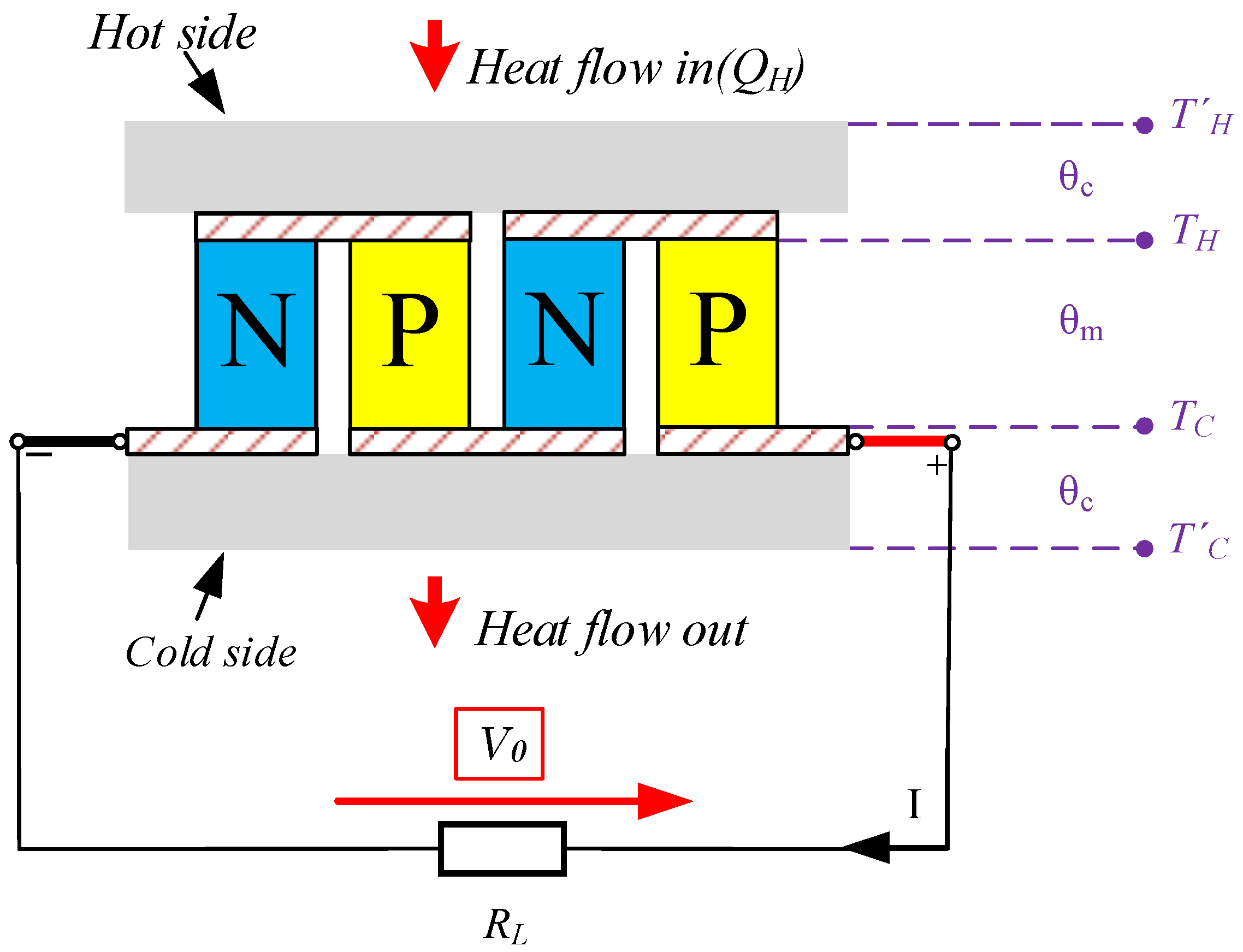
- The Seebeck coefficient , which depends on the thermoelectric materials used to manufacture p-n semiconductors.
- The electrical resistance , comprising the electrical resistance of the p-n semiconductors and contacts used to connect the TEG to an electrical load.
- The internal thermal resistance and the contact thermal resistance , used to interface the TEG to a thermal source of energy.
2. Fully Electrical Modeling of a TEG under Different Operating Conditions
2.1. Constant Temperature Gradient Conditions
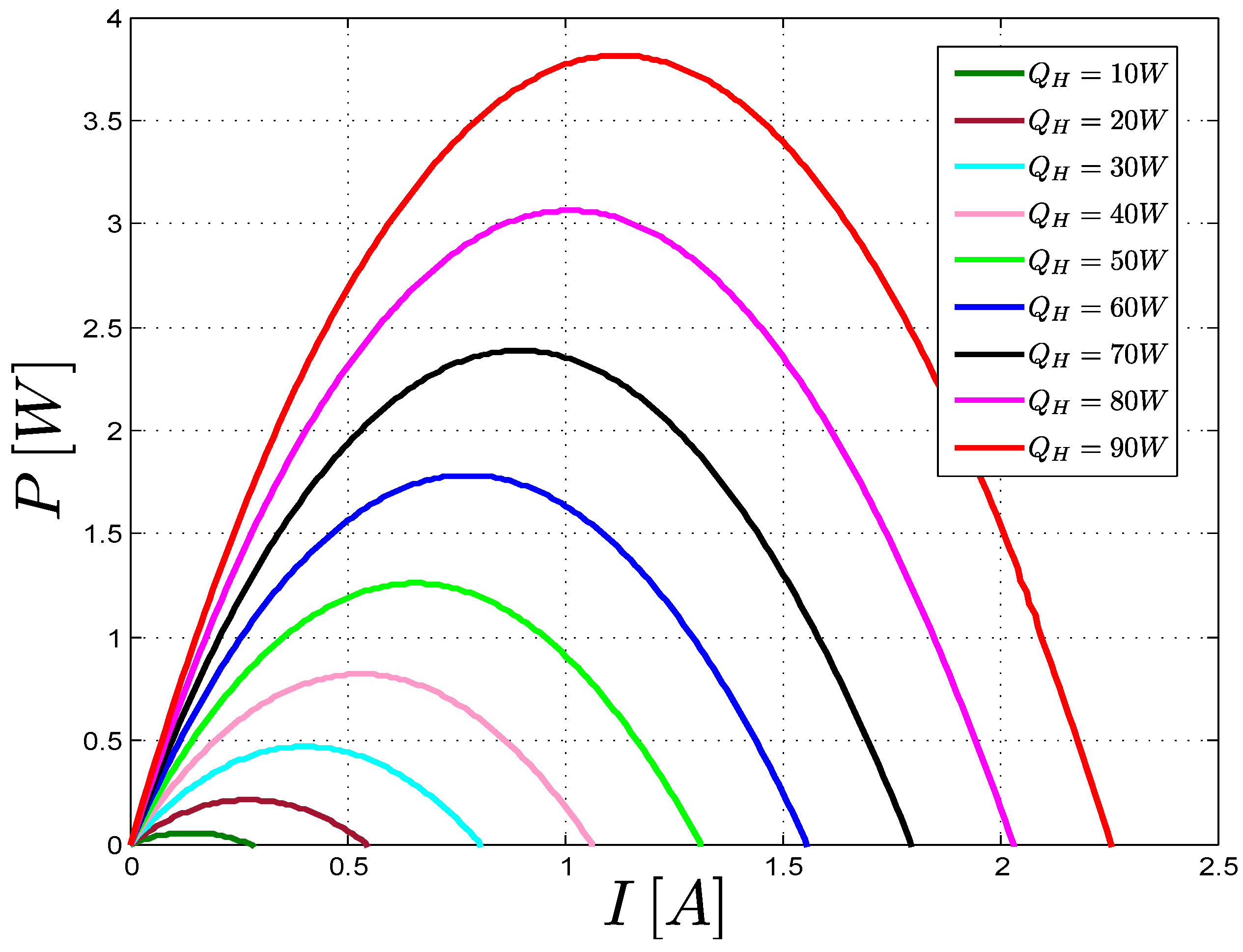
2.2. Constant Heat Flow Conditions
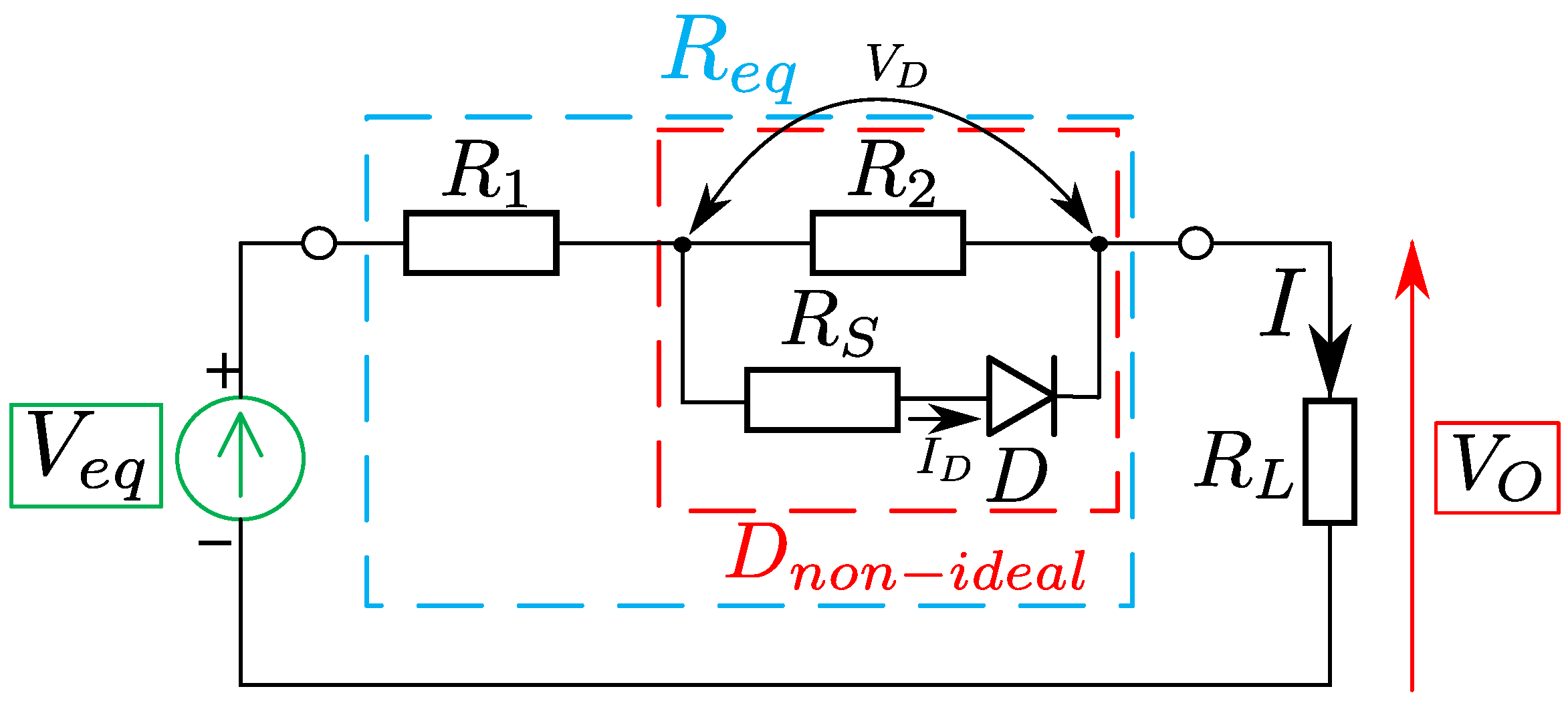
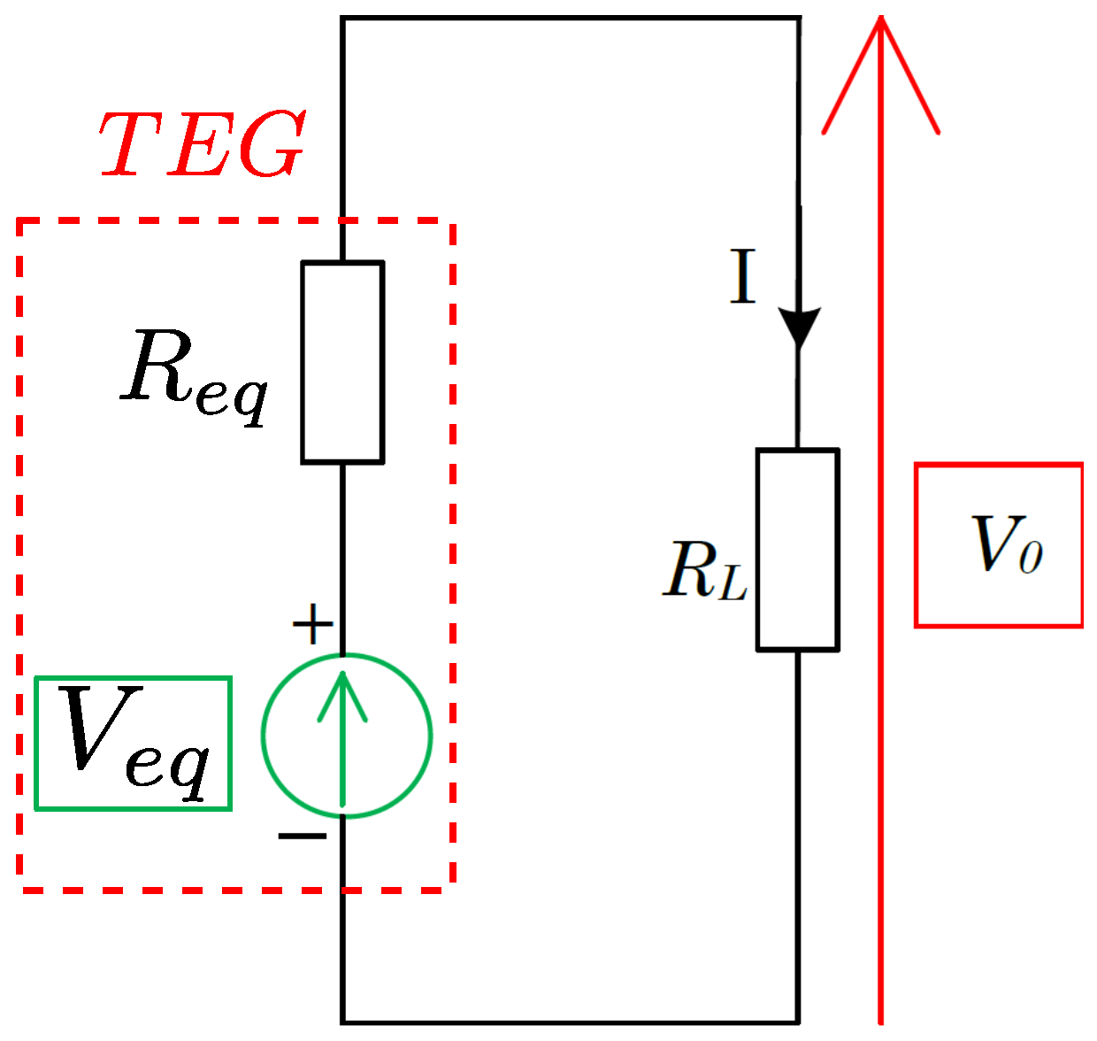
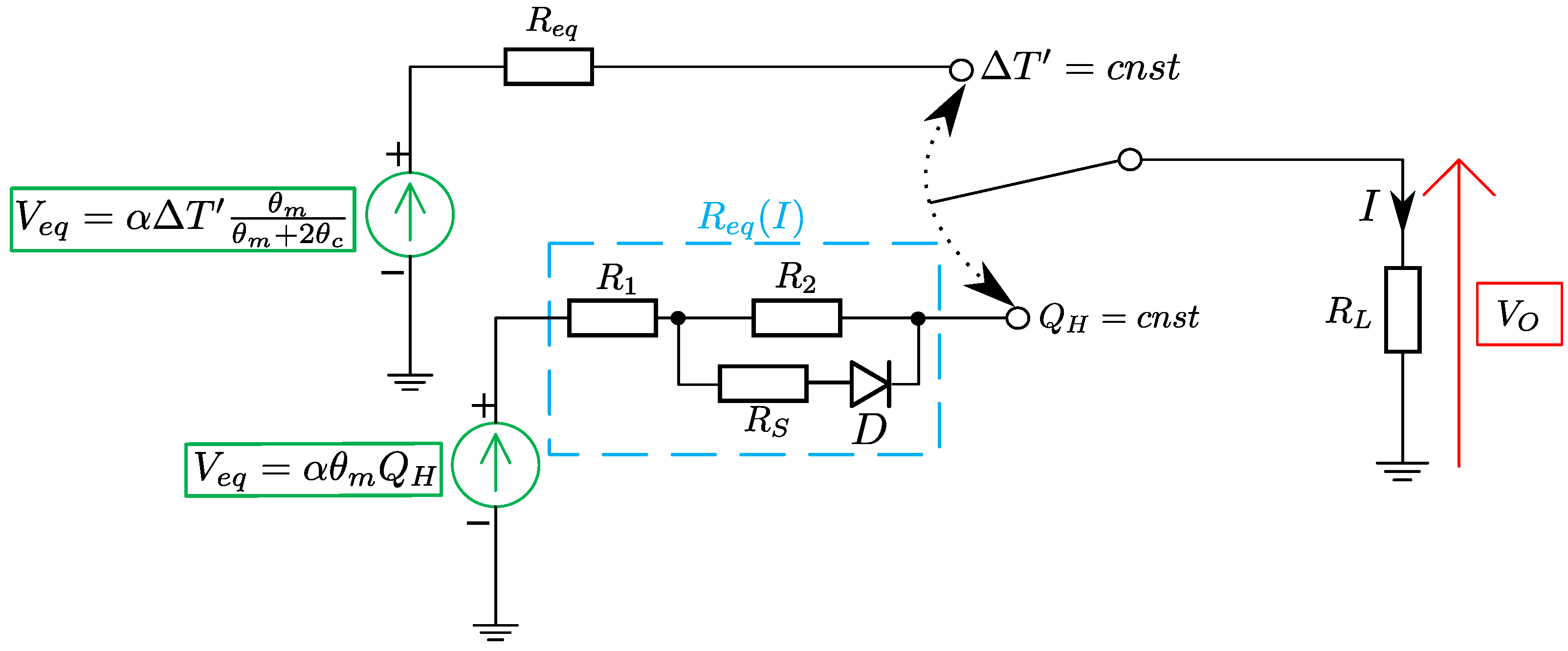
3. Equivalent Electrical Circuits of a TEG: Static Operating Conditions with Constant /
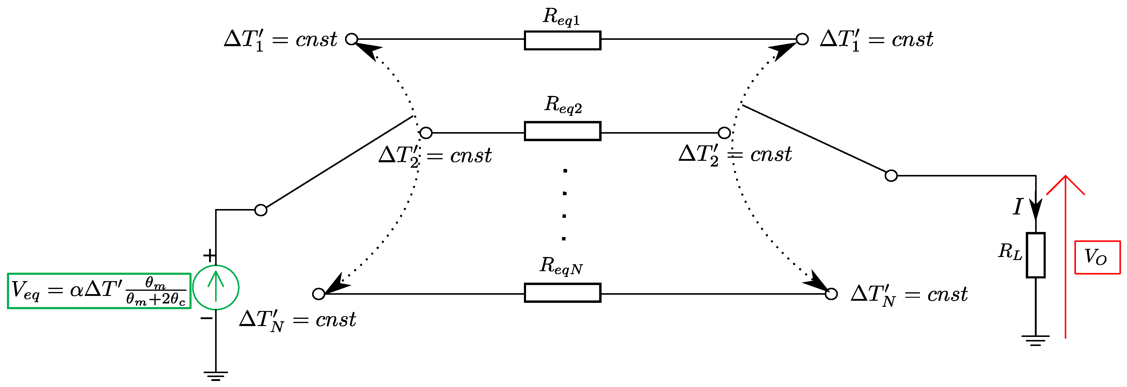
3.1. Constant Temperature Gradient Conditions
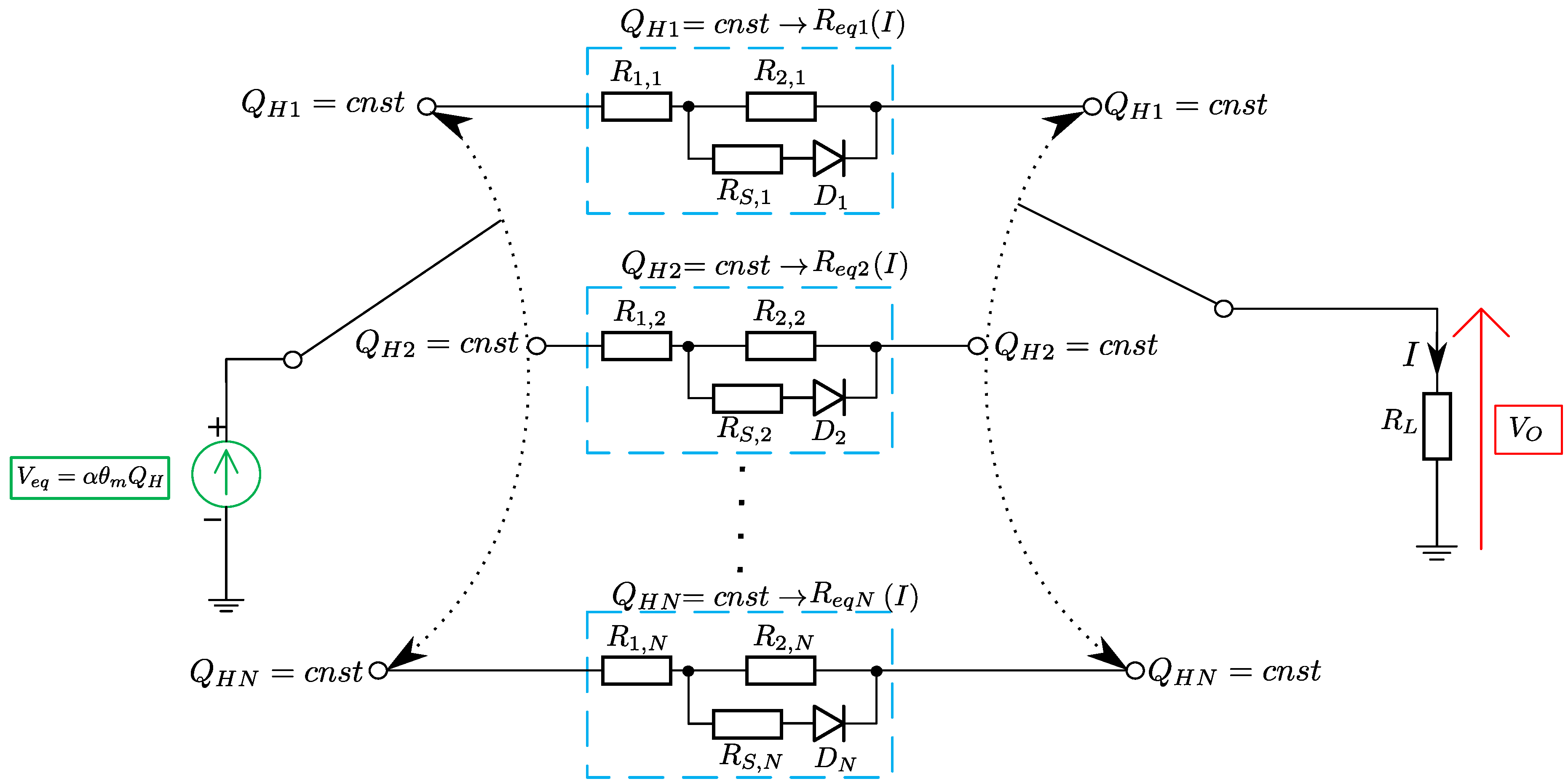
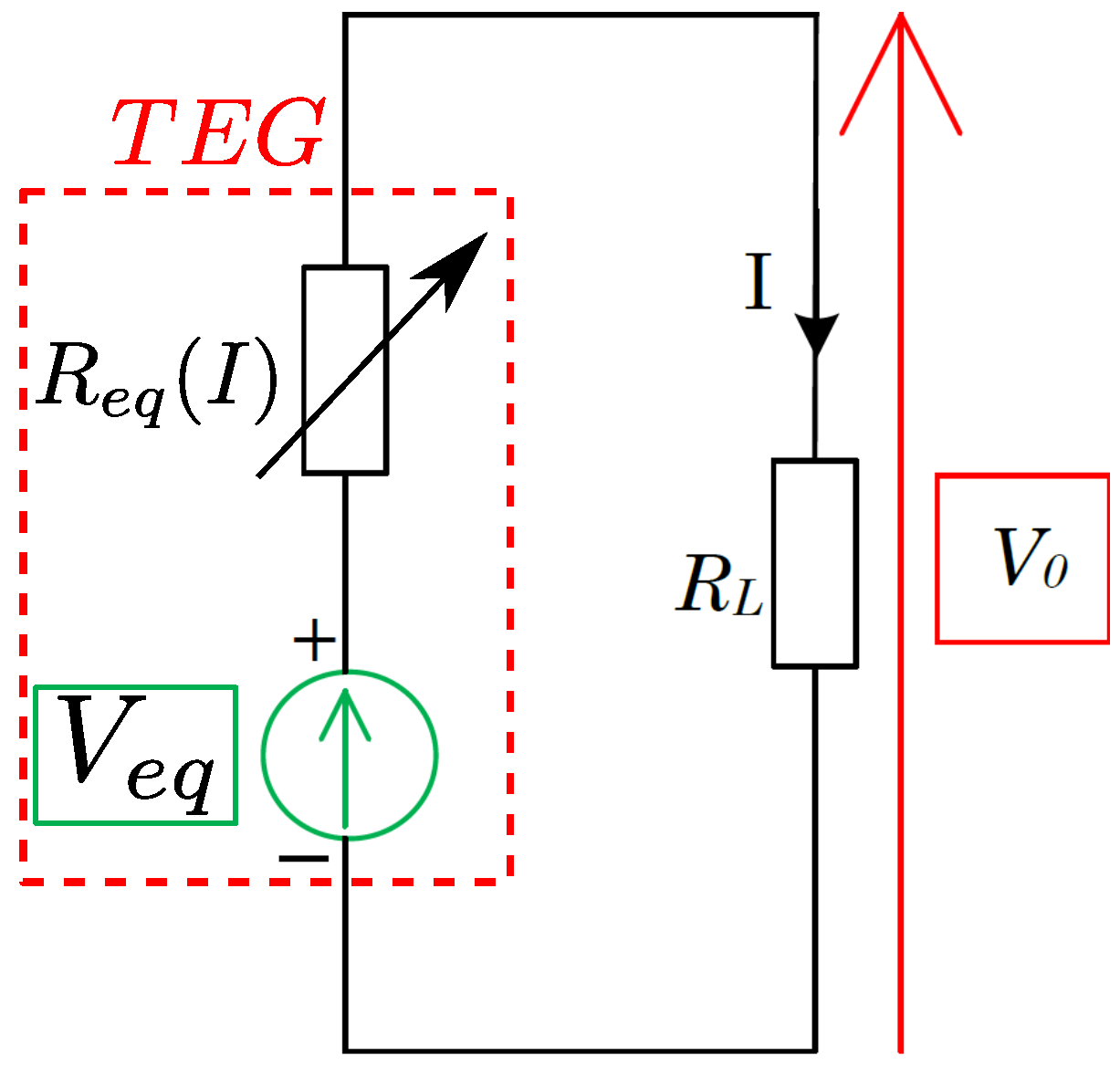
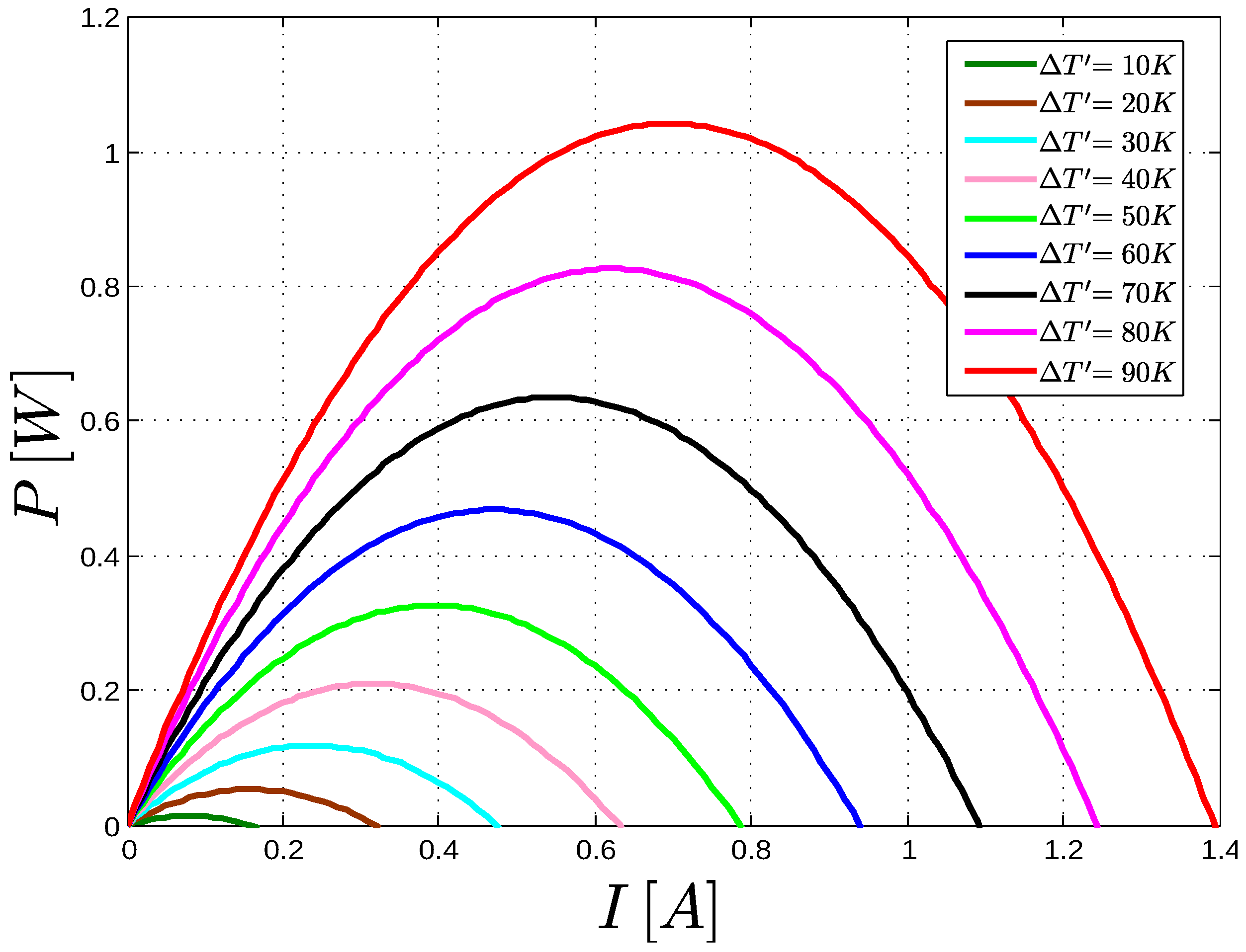
3.2. Constant Heat Flow Conditions
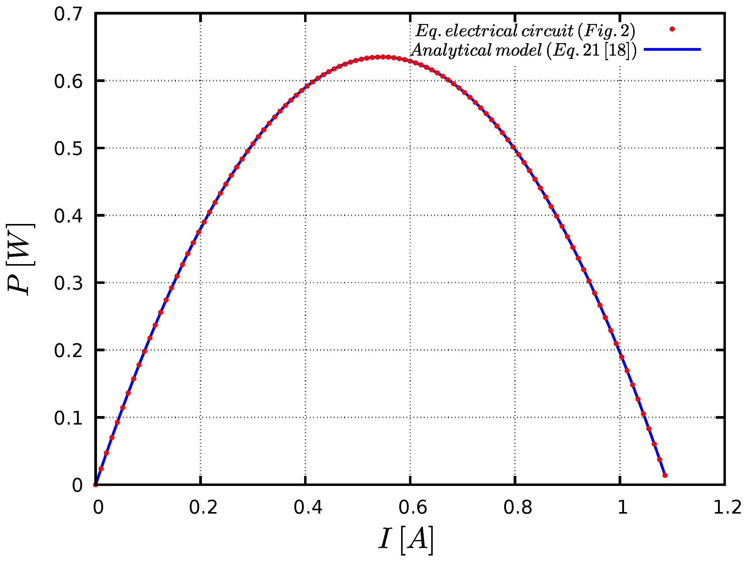
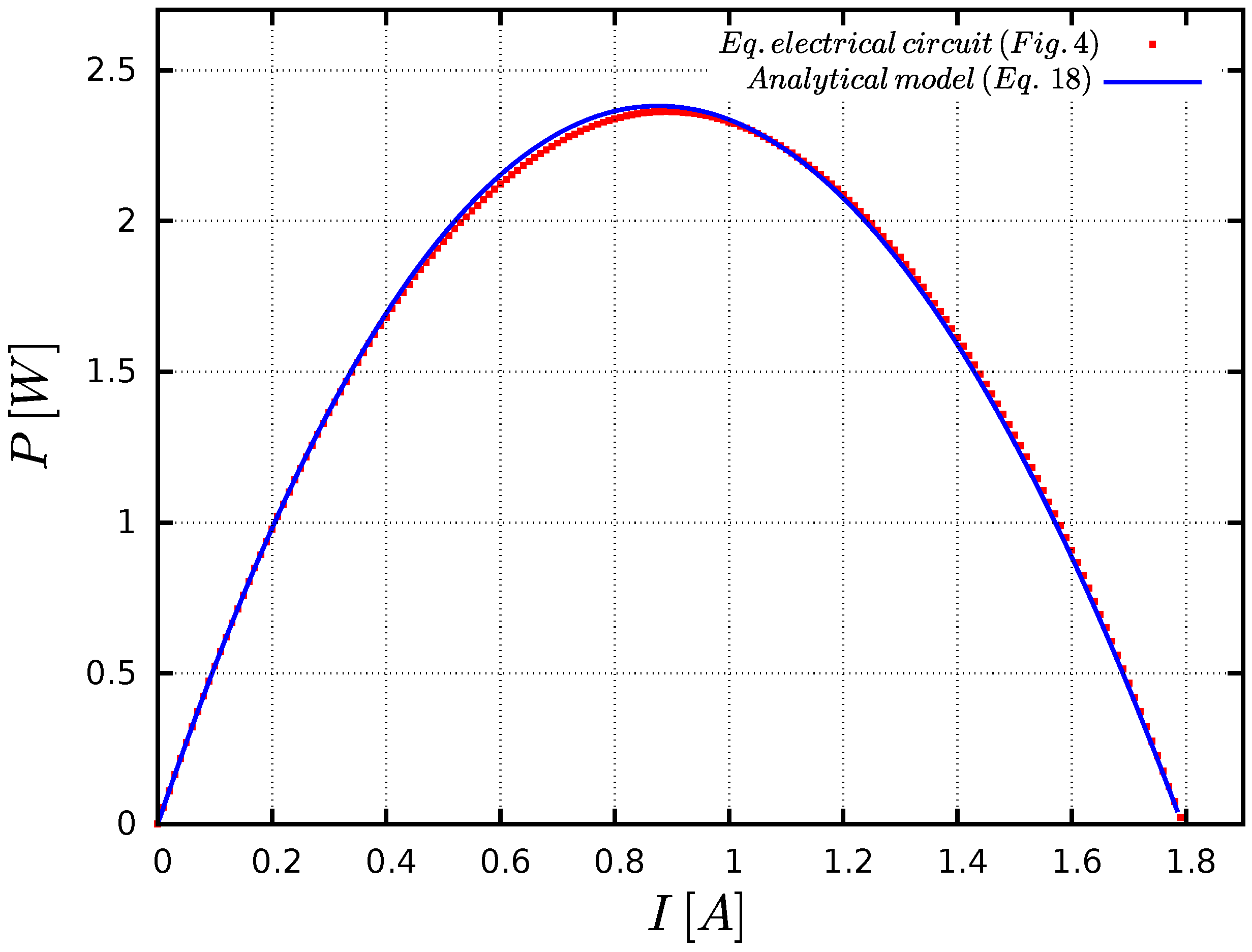
3.3. Validation of Equivalent Electrical Circuits through Simulation
4. Equivalent Electrical Circuits of TEG: Dynamic Operating Conditions or
5. Conclusions
Author Contributions
Conflicts of Interest
References
- Mitcheson, P.D.; Yeatman, E.M.; Rao, G.K.; Holmes, A.S.; Green, T.C. Energy harvesting from human and machine motion for wireless electronic devices. Proc. IEEE 2008, 96, 1457–1486. [Google Scholar] [CrossRef] [Green Version]
- Yang, Y.; Wei, X.-J.; Liu, J. Suitability of a thermoelectric power generator for implantable medical electronic devices. J. Phys. D: Appl. Phys. 2007, 40, 5790. [Google Scholar] [CrossRef]
- Su, S.; Chen, J. Simulation investigation of high-efficiency solar thermoelectric generators with inhomogeneously doped nanomaterials. Trans. Ind. Electron. 2015, 62, 3569–3575. [Google Scholar] [CrossRef]
- Roth, R.; Rostek, R.; Cobry, K.; Köhler, C.; Groh, M.; Woias, P. Design and characterization of micro thermoelectric cross-plane generators with electroplated, and reflow soldering. J. Microelectromech. Syst. 2014, 23, 961–971. [Google Scholar] [CrossRef]
- Dewan, A.; Ay, S.U.; Karim, M.N.; Beyenal, H. Alternative power sources for remote sensors: A review. J. Power Sources Elsevier 2014, 245, 129–143. [Google Scholar] [CrossRef]
- Koplow, M.; Chen, A.; Steingart, D.; Wright, P.K.; Evans, J.W. Thick film thermoelectric energy harvesting systems for biomedical applications. In Proceedings of the 5th IEEE International Summer School and Symposium on Medical Devices and Biosensors, Hong Kong, China, 1–3 June 2008; pp. 322–325.
- Kappel, R.; Pachler, W.; Auer, M.; Pribyl, W.; Hofer, G.; Holweg, G. Using thermoelectric energy harvesting to power a self-sustaining temperature sensor in body area networks. In Proceedings of the IEEE International Conference on Industrial Technology (ICIT), Cape Town, South Africa, 25–28 February 2013; pp. 787–792.
- Leonov, V. Thermoelectric energy harvesting of human body heat for wearable sensors. IEEE Sens. J. 2013, 13, 2284–2291. [Google Scholar] [CrossRef]
- Ahiska, R.; Mamur, H. Design and implementation of a new portable thermoelectric generator for low geothermal temperatures. Renew. Power Gener. IET 2013, 7, 700–706. [Google Scholar] [CrossRef]
- Hsu, C.T.; Yao, D.J.; Ye, K.J.; Yu, B. Renewable energy of waste heat recovery system for automobiles. J. Renew. Sustain. Energy 2010, 2, 013105. [Google Scholar] [CrossRef]
- Carstens, T.; Corradini, M.; Blanchard, J.; Ma, Z. Thermoelectric powered wireless sensors for spent fuel monitoring. In Proceedings of the 2nd IEEE International Conference on Advancements in Nuclear Instrumentation Measurement Methods and their Applications (ANIMMA), Ghent, Belgium, 6–9 June 2011; pp. 1–6.
- Kim, R.Y.; Lai, J.S.; York, B.; Koran, A. Analysis and design of maximum power point tracking scheme for thermoelectric battery energy storage system. IEEE Trans. Ind. Electron. 2009, 56, 3709–3716. [Google Scholar]
- Yazawa, K.; Shakouri, A. Cost-efficiency trade-off and the design of thermoelectric power generators. Environ. Sci. Technol. 2011, 45, 7548–7553. [Google Scholar] [CrossRef] [PubMed]
- Nemir, D.; Beck, J. On the significance of the thermoelectric figure of merit z. J. Electron. Mater. 2010, 39, 1897–1901. [Google Scholar] [CrossRef]
- Karami, N.; Moubayed, N. New modeling approach and validation of a thermoelectric generators. In Proceedings of the 2014 IEEE 23rd International Symposium on Industrial Electronics (ISIE), Istanbul, Turkey, 1–4 June 2014; pp. 586–591.
- Bond, M.; Park, J.D. Current-sensorless power estimation and MPPT implementation for thermoelectric generators. IEEE Trans. Ind. Electron. 2015, 62, 5539–5548. [Google Scholar] [CrossRef]
- Siouane, S.; Jovanovic, S.; Poure, P. Influence of contact thermal resistances on the Open Circuit Voltage MPPT method for thermoelectric generators. In Proceedings of the 2016 IEEE International on Energy Conference (ENERGYCON), Leuven, Belgium, 4–8 April 2016.
- Siouane, S.; Jovanovic, S.; Poure, P. Fully electrical modeling of thermoelectric generators with contact thermal resistance under different operating conditions. J. Electron. Mater. 2017, 46, 40–50. [Google Scholar] [CrossRef]
- Montecucco, A.; Siviter, J.; Knox, A.R. Constant heat characterisation and geometrical optimisation of thermoelectric generators. Appl. Energy Elsevier 2015, 149, 248–258. [Google Scholar] [CrossRef]
- Dousti, M.J.; Petraglia, A.; Pedram, M. Accurate electrothermal modeling of thermoelectric generators. In Proceedings of the 2015 Design, Automation & Test in Europe Conference & Exhibition (DATE’15), Grenoble, France, 9–13 March 2015; pp. 1603–1606.
- Siouane, S.; Jovanovic, S.; Poure, P. Equivalent electrical circuit of thermoelectric generators under constant heat flow. In Proceedings of the IEEE 16th International Conference in Environment and Electrical Engineering (EEEIC), Florence, Italy, 7–10 June 2016; pp. 1–6.
- Ortiz-Conde, A.; Francisco, J.G.; Muci, J. Exact analytical solutions of the forward non-ideal diode equation with series and shunt parasitic resistances. J. Solid-State Electron. 2000, 44, 1861–1864. [Google Scholar] [CrossRef]


| Parameter | Value |
|---|---|
| N | 127 |
| α | 0.0531876 (V/K) |
| 1.6 (Ω) | |
| 1.498 (K/W) | |
| 0.45 (K/W) | |
| 298 (K) | |
| 368 (K) | |
| 70 (W) |
| Parameter | Value | |
|---|---|---|
| (V) | 5.5787409888 | |
| (A) | 1.793212008160477 | |
| (V) | 2.720928218743778 | |
| (A) | 0.8749283875525364 | |
| (Ω) | 0.6648702522882615 | |
| (Ω) | 2.776437457558251 | |
| (A) | ||
| (Ω) | ||
| n | ||
| (nA) | 300 |
© 2017 by the authors. Licensee MDPI, Basel, Switzerland. This article is an open access article distributed under the terms and conditions of the Creative Commons Attribution (CC BY) license ( http://creativecommons.org/licenses/by/4.0/).
Share and Cite
Siouane, S.; Jovanović, S.; Poure, P. Equivalent Electrical Circuits of Thermoelectric Generators under Different Operating Conditions. Energies 2017, 10, 386. https://doi.org/10.3390/en10030386
Siouane S, Jovanović S, Poure P. Equivalent Electrical Circuits of Thermoelectric Generators under Different Operating Conditions. Energies. 2017; 10(3):386. https://doi.org/10.3390/en10030386
Chicago/Turabian StyleSiouane, Saima, Slaviša Jovanović, and Philippe Poure. 2017. "Equivalent Electrical Circuits of Thermoelectric Generators under Different Operating Conditions" Energies 10, no. 3: 386. https://doi.org/10.3390/en10030386