1. Introduction
The oxyfuel combustion technology was introduced in the late eighties to target the increasing demand for controlling the CO
2 and NO
x production in industrial combustion systems. In this technology, the fuel is combusted in an almost pure oxygen atmosphere instead of using air. This provides the mean for a CO
2 sequestration from the flue gases [
1]. This combustion technology was initially promoted and studied for the usage in coal-fired power plants and coal-combustion applications [
2,
3]. Later on, this technology became rapidly popular for use in other applications, as academic attention was also attracted to the subject in order to provide a better understanding and to develop modification methods [
4]. In addition, fundamental research was carried out by Argonne National Laboratory (ANL) with the study on a pilot scale furnace equipped with an oxyfuel burner [
5,
6,
7]. Later, the International Flame Research Foundation (IFRF) carried out major research in this area, with usage of an oxy-coal combustor with a flue gas recirculation (FGR) system.
In 2005, Buhre et al. [
2] highlighted the importance of employing oxyfuel systems as an approach for CO
2 sequestration. They provided a comprehensive research review of previous work that had been carried out as well as the status of the technology at that time. In the same year, Wall et al. [
8] pointed out the importance of the role of recycled flue gases inside the combusting chamber. They claimed that these can control the flame temperature and compromise the lack of the flue gas volume (N
2) in an oxyfuel system. In 2007, the flame stability and NO
x emissions from oxy-fuel combustion was investigated by Kim et al. [
9], in an experimental study. The system in this study was also equipped with a FGR system. They reported that the oxyfuel combustor has the best flame stability. Another experimental work was done by Andersson et al. [
10] which investigated the combustion chemistry in air-fuel and oxyfuel combustion systems. The study was done on a 100 kW test unit and the results showed that oxyfuel produces up to 30% less NO
x emissions compared to an identical air-fuel combustion system. In 2010, Toftegaard et al. [
11] performed an extensive literature study on the subject of oxyfuel combustion. They concluded that a large lack of research exists in both pilot and plant testing on the issues related to oxyfuel combusting systems. A more extensive literature survey about oxyfuel combustion is presented in the work by Ghadamgahi et al. [
12] and Wall et al. [
13].
In the meantime, while many theoretical and laboratory studies were carried out on the subject, the fast development of computational simulations led to a new trend of using them to study the complicated issues related to combustion. Examples of the numerical studies on oxy-fuel combustion systems are given in references [
14,
15,
16]. The focus of these studies was to develop and validate the proper computational models for combustion and radiation. More specifically, Johansson et al. [
14] compared four different radiation models to study the accuracy and the relevance of using them to simulate an oxy-fired boiler. They reported that the weighted sum of the gray gases model (WSGGM) was the most accurate model to use for these applications. In 2012, Hjärtstam et al. [
15] used the measured data of a 100 kW oxyfuel unit to investigate the effect of a non-gray radiation model on the predicted results. They reported that the non-gray model predicts acceptable results. Additionally, the SLFM combustion model was employed in this work, regarding the work done by Galletti et al. [
17], and Ghadamgahi et al. [
12]. In 2013, Galletti et al. [
17] compared the predicted results from computational fluid dynamics (CFD) calculations for an oxy-natural gas combustion system, to the experimental results of a 3 MW semi-industrial furnace. They observed that the sub model, which considered a fast chemistry, was inaccurate for predicting the temperature magnitudes. Also, Ghadamgahi et al. [
12] compared the predicted results from two CFD models, with and without chemical equilibrium, with experimental data, and the latter showed a better agreement [
12]. A turbulence model of realizable
k-ε was used according to the works by Liu et al. [
18] and Ghadamgahi et al. [
12]. Also, in 2016 Aziz et al. [
19] used the
k-ε turbulence model to investigate the palm kernel shell (PKS) co-firing of a 300 MWe pulverized coal-fired power plant [
19]. It is also mentioned in the work by Filipponi et al. [
20] that the realizable
k-ε model gives more accurate results compared to the results from standard
k-ε [
20].
According to the literature above, one can consider the bullet points below as the main known advantages of oxyfuel combustion systems:
Although, with increasing the usage of this technology some operational issues were also noticed. Examples of research that pointed out these issues were done by Buhre et al. [
2] and Fredriksson et al. [
21]. In Buhre et al. [
2], the authors identified some problems associated with the use of oxyfuel combustion with respect to heat transfer, flame stability, and gaseous emissions. In addition, Fredriksson et al. [
21] investigated the effect of air infiltration into the chamber, on the total NO
x formation. They reported that the sharp temperature gradient in the flame area produces a large amount of NO
x in the case of air infiltration. This consequently leads to a non-uniform scale formation on the slabs.
One of the modified versions of the conventional oxyfuel systems was the flameless oxyfuel combustion systems [
4]. These systems also use pure oxygen as the oxidant, but the difference to normal oxyfuel burners is the use of a special burner design and a high (near-sonic) injection velocity for both fuel and oxygen. The design of the burner, including the diameter and distance of the nozzles, promotes a high internal flue gas recirculation (IFGR) [
4,
22]. In the case of correct adjustments, the result is the production of a volumetric strained flame with a spread temperature distribution and a low concentration of oxygen and nitrogen inside the combustion chamber [
22].
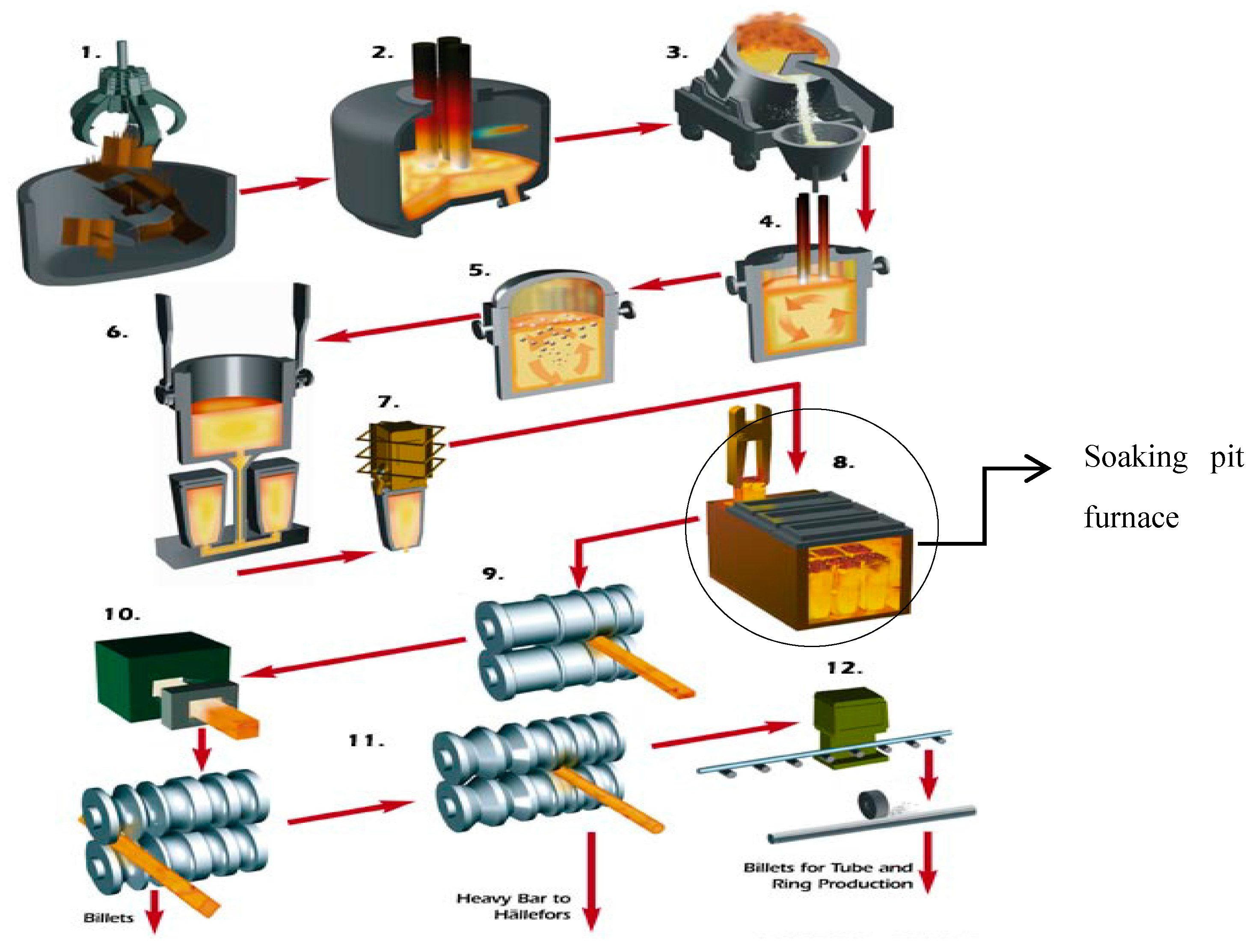
Shortly after the commercialization of this technology, it became a common practice in many steel industries, such as in walking beam and catenary furnaces at Outokumpu (Sweden) in 2003 [
4], nine soaking pit furnaces at Arcometal (France) in 2005 [
4], a rotary heart furnace in ArcelorMittal Shelby (OH, USA) in 2007 [
4] and soaking pit furnaces in Ovako Sweden AB, in Hofors (Sweden) [
4]. Beside these applications, a few academic studies were also performed to provide a better understanding of the practical issues and modeling tools. In 2006, Vesterberg et al. [
23] listed the most important findings they observed by studying 10 full-scale industrial users of the flameless oxyfuel technique in reheating and annealing furnaces. Those are: a more uniform heating process, shorter heating cycles, and ultra-low emissions of NO
x even with the existence of ingress air. In the work by Krishnamurthy at al. [
24] different burner types, such as flameless oxyfuel burners and high temperature air combustion (HiTAC) burners, were evaluated with respect to their thermal efficiency, inflame temperature distribution, heat flux, gas composition, and NO
x emissions for different levels of in-leakages of air. They concluded that the flameless burners provide a higher energy utilization efficiency, and a better temperature uniformity and heat flux profile, compared to traditional burners.
In 2007, Krishnamurthy et al. [
25] used a semi-industrial furnace to investigate the NO
x formation for flameless oxyfuel combustion. They examined different burners, including a flameless oxy-propane burner to provide a comparative end-result. The comparisons show many advantages of using the flameless oxyfuel burners in comparison to traditional burners, such as a lower NO
x formation and a better temperature uniformity [
25]. Later in 2016, Ghadamgahi et al. [
12] used the experimental data from Krishnamurthy et al. [
25] to compare three different CFD models and to validate the predictions for simulations of a flameless oxyfuel combustion [
12]. These models were later used to simulate a full-scale soaking pit furnace and the predicted results were compared with experimental results presented by Ghadamgahi et al. [
26].
Although these few studies were very useful to help understand and model the complicated case of using the flameless oxy-fuel technique, there is a large lack of studies on the role of operational parameters on the functioning condition of these burners. This is especially essential for industrial applications; to understand the effect of important operational parameters, such as the oxygen/fuel (lambda), efficiency, and temperature profile, on the combustion performance.
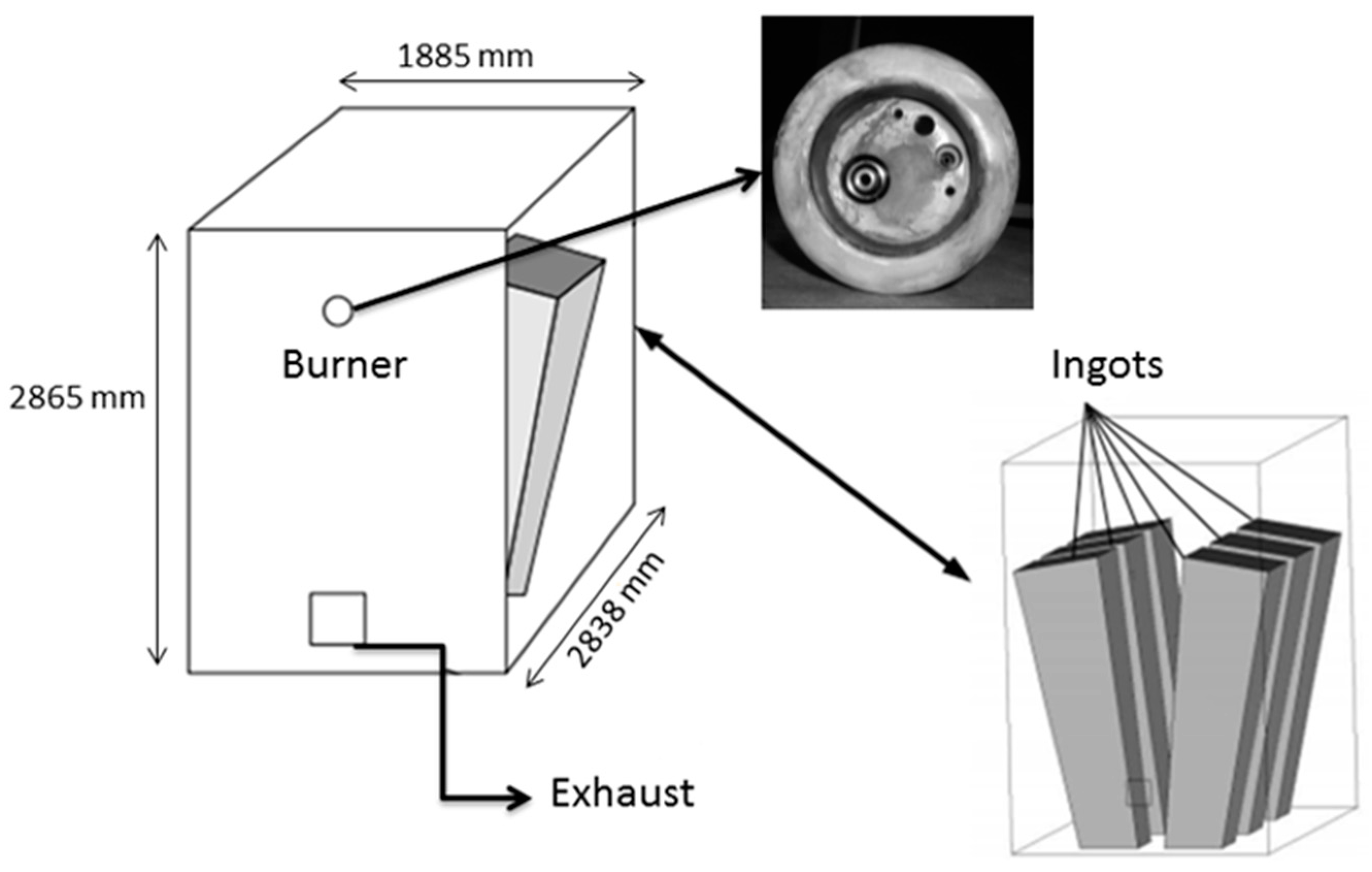
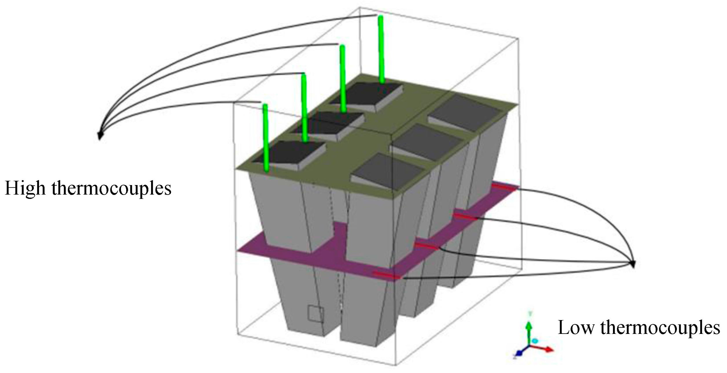
In this study, the validated models from the work by Ghadamgahi et al. [
12,
26] are used to simulate a full-size soaking pit furnace containing ingots, since the differences in the geometries is negligible. Simulations have been performed for six cases, using different magnitudes of the lambda value (inlet oxygen values). The validation was previously performed by comparing the predicted results with those taken from the experiments on a soaking pit furnace, equipped with a flameless oxyfuel burner, in Ovako Sweden AB [
26]. The results from these simulations are used to compare these cases and to investigate the effect of the lambda value on the operational condition of a furnace when using a flameless oxyfuel combustion. Thus, to link an easy controlled parameter to temperature uniformity is of great practical value for the industry. In addition, a new definition of furnace efficiency is proposed. It considers the operational costs of a furnace besides the thermal costs. These operational costs are solely due to the design and operational conditions of the furnace.
2. Mathematical Models
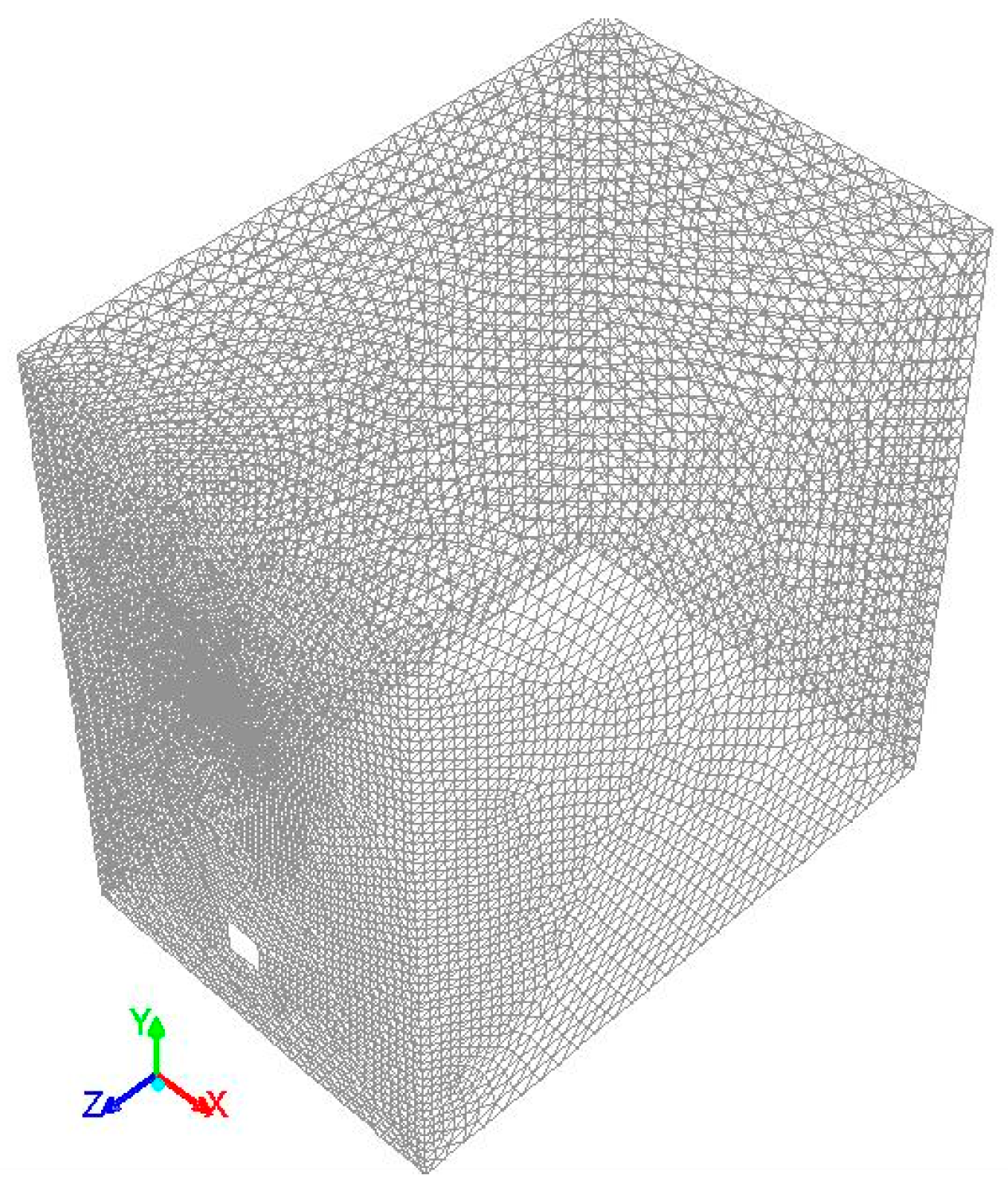
A 3-dimensional mathematical model was developed to simulate the combustion in Ansys Fluent 16.0 (Producs 16, Ansys, Inc.,
http://www.ansys.com/). The following assumptions were considered to solve the problem:
The flue gas mixture was assumed to behave like a perfect gas mixture.
The condition was assumed to be steady state and therefore independent of time.
The Lewis number for all the gas species was assumed to be one.
The flow was assumed to be fully turbulent.
The diffusion coefficients for all the gaseous products were assumed to be equal.
All the external forces, except the gravity, were neglected.
The flow was assumed to be incompressible in the chamber.
Infiltration of air was assumed to be negligible and NOx products were ignored.
Combustion was assumed departed from the chemical equilibrium.
A second-order upwind discretization scheme was used to solve the governing equation.
The governing equations were solved according to the assumptions above. Specifically these equations are:
Energy balance equation:
where
is the velocity vector (m/s),
is the density (kg/m
3) and
is the stress tensor. Furthermore,
and
are the gravitational body forces and the pressure (Pa), respectively. In addition,
represents the thermal conductivity (W/m·K), and
defines the heat capacity at a constant pressure (J/kg·K) [
26]. Also
counts for any volumetric heat sources.
Regarding the incompressible behaviour of the flow, the Navier Stokes equation is solved, which can be written as follows:
where the parameter
represents the gravity and ω is thermodynamic work on the system. Furthermore, the parameter
is the kinematic viscosity.
The realizable
k-ε turbulence model was used to solve the Navier-Stokes equations and to model the turbulence. The validity of this sub-model for such problems is intensely argued in the work by Ghadamgahi et al. [
12]. The turbulent kinetic energy (
k) and the turbulent dissipation rate (ε) were solved as shown in Equations (5) and (6):
where
.
And σ
k = 1.0, σ
ε = 1.2,
C2 = 1.9,
C1ε = 1.44, and
is described by Equation (7).
According to the configuration of the burner, a non-premixed combustion with the mixture fraction (
) is considered. The mixture fraction is introduced as follows:
where
stands for the
ith species mass fraction and the subscript
ox and
fuel stand for the oxidizer stream and fuel stream, respectively. The combustion is calculated by using the SLFM to solve the PDF. This model considers the non-equilibrium effects of the combustion. This selection of a sub-model for reaching an accurate prediction for combustion is explained and argued in the work by Ghadamgahi et al. [
12]. In this approach, the thermochemistry parameters are a function of the mixture fraction and the strain rate or Dissipation rate (
):
where
is the diffusion coefficient.
Therefore, the following formulation is used to calculate the thermochemical parameters:
where
represents the species mass fractions and temperature while
represents the stoichiometric dissipation rate [
12].
For modeling the radiation, the DO radiation model with the WSGGM is used to solve the general radiative transfer equation (RTE). The set-up for using this method for the special case of oxy-fuel has been widely investigated in the literature [
14,
16,
27,
28,
29].
The RTE over the radiative path of
S and a spectral averaging over a band
k is described as follows:
where the over-bar stands for a spectral average over a band
k, the index
i refers to the spatial discretization, and
can be expressed as follows:
where
is the absorption coefficient [
12].


