A Cyber Physical Model Based on a Hybrid System for Flexible Load Control in an Active Distribution Network

Abstract

To strengthen the integration of the primary and secondary systems, a concept of Cyber Physical Systems (CPS) is introduced to construct a CPS in Power Systems (Power CPS). The most basic work of the Power CPS is to build an integration model which combines both a continuous process and a discrete process. The advanced form of smart grid, the Active Distribution Network (ADN) is a typical example of Power CPS. After designing the Power CPS model architecture and its application in ADN, a Hybrid System based model and control method of Power CPS is proposed in this paper. As an application example, ADN flexible load is modeled and controlled with ADN feeder power control by a control strategy which includes the normal condition and the underpowered condition. In this model and strategy, some factors like load power consumption and load functional demand are considered and optimized. In order to make up some of the deficiencies of centralized control, a distributed control method is presented to reduce model complexity and improve calculation speed. The effectiveness of all the models and methods are demonstrated in the case study.

1. Introduction

With the rapid development of network technology, and increasing requirements for accuracy and efficiency of industry control, the industry needs to strengthen information acquisition, application and coordination control with the hierarchy-distributed control system. Hence, a new concept of Cyber Physical Systems (CPS) is proposed to promote the tight integration of control, communication, information, industry process, and reveal the integration mechanism of the real and virtual world [1].

CPS stems from embedded systems. To satisfy the performance requirement of spatial layout and power consumption, the traditional embedded system focuses on the optimal resource utilization of hardware and software [2]. However, the embedded system in CPS concentrates on the interaction with the real physical system (controlled object), and focuses on problems such as concurrent event which cannot be perceived if the controlled object is too complicated [3].

Several research results on CPS have been presented. The purpose of them is to explore principle of interaction between cyber and physical systems, promote the system ability of sensing, analysis, decision and control. For example, when operating cardiac surgery by robot arms, the arms should vibrate with the heart at the same frequency to maintain relative rest [4]. CPS models are built in [5,6] for fuel management and airspace management of aviation systems to optimize flight operation.

A power system meets the basic form of CPS. Especially after the smart grid and micro grid are presented, intellectualization and informatization cover almost all parts of the power system from source side to load side, and then the relationship and coordination among these parts are tighter. So the power system has had basis and actual demand to construct a complete CPS.

There are a few researches of CPS in the power system at present. Most of them focus on the influence brought from the information system (including the secondary system and the communication network) to the primary system. For example, in the aspect of reliability of relay protection, cyber factors like fault rates of logical nodes and logical connections in IEC61850 based substation automation system [7] and the fault rate of a communication link [8] are all considered in a traditional physical device reliability assessment. In the aspect of communication network, information system elements including communication routing [9], network time delay [10] and system observability [11] have been integrated into the primary system to analyze stability margin. There are also some researches about information security in the power system, such as information attack occurring in SCADA [12] and substation automation [13]. To test the interaction between the information and primary system, several simulation platforms have been built such as INSPIRE [14], GECO [15], and TASSCS [16].

Besides the influence of information system, some researches consider that continuity and discrete are the main attributes of Cyber and Physical system respectively. So they try to rebuild power grid model according to Hybrid System theory which describes both the continuous dynamic and discrete state, then the object-oriented hybrid power system model library is developed [17], and sliding mode control based on the hybrid models can be applied to DG integrated shipboard power grid [18].

The main target of the Active Distribution Network (ADN) is to promote Distributed Generation (DG) utilization and reduce energy from the external system [19]. In ADN, the control system coordinate with the primary system, complex energy flow, and information flow coexist when operating. Hence, ADN is suitable to be a study object for Power CPS. But, most of the existing ADN researches is on DGs control, and load control has still not been fully considered. The hierarchical control system in [20] is not only used in DG power control, but also in load control.

The load control is always a hot point for research. For instance, the relationship of refrigerators and the frequency in the micro grid are explored in [21]. A Model Predictive Control (MPC) based method is proposed in [22] to optimize the profit of power demand in the commercial office building. From the point of CPS, literature [23] introduces a method of a Real-Time Physical System to reduce system instantaneous power consumption by adjusting the load coincidence factor.

There are several types of model which can be used in CPS to solve different problems. The Hybrid System is a typical one which can reflect CPS connotations, and can be used in control. This paper builds a Hybrid System based modeling structure for Power CPS which is beneficial for analyzing the interactive mechanism between information and the primary system. Then according to the modeling structure, an integration model method and its application are studied to optimally and predictively control the power system by an example of a flexible load control in ADN.

The rest of the paper is organized as follows: Section 2 describes the composition and characteristics of the Power CPS model, and designs application schemes in ADN. Section 3 presents a Hybrid System based CPS model and the control strategy for an ADN flexible load. Aiming at some shortages in Section 3, a distributed ADN flexible load control method is proposed in Section 4. All the models and methods are applied to simulated examples in Section 3 and Section 4 respectively. Section 5 provides concluding remarks.

2. Power CPS Model and Its Application in ADN

Power CPS technical features and key techniques have been summarized in [24]. Among these key techniques, the Cyber Physical model is the most basic work. Figure 1 shows the relationship between technical features and model in Power CPS.

According to the three features in Figure 1, the Power CPS model can be classified into two kinds: “Control Model” and “Information Model”. The “Information Model” corresponds to Feature (3), and this type of model mainly studies a uniform information description mode which can be applied in information exchange after combining with an information transmission structure including the model mapping method and communication protocol.

The “Control Model” reflects Features (1) and (2), and this type of model focuses on promoting the interaction and eliminating the heterogeneity between the primary and the information system in the power grid.

2.1. Control Model Based on Hybrid System

Compared with the Information Model, the ‘Control Model’ undertakes the main tasks of Power CPS control. As is shown in Figure 1, the ‘Control Model’ strengthens the integration of cyber and physical in two aspects.

(1) Integrating physical process and control process

This aspect reflects the interaction between physical characteristic and the control input of primary devices. During the operation, the state variable and output of the primary device change with time continuously, but the control input can be seen as a kind of disturbance which interrupts and changes the current’s continuous dynamic. No matter how the input is transmitted to the primary device, the input affects the device’s physical process in a certain time interval, thus the continuous dynamic switches to new states discretely. Therefore, when the control input is being generated to control a device, continuous process of this device and discrete state switching caused by input should both be considered.

(2) Integrating of primary system and information system

This aspect describes the interaction between the information system, control process and primary system. Where, the information system not only refers to the nodes which may be traversed by information flow, but also the sequence and time of different information flow. So the influence caused by the information system can be represented as topology and sequential logic, and incorporated in the ‘integrating of physical process and control process’ introduced above. Figure 2 illustrates the relationship between two aspects of ‘integrating’ in the ‘Control Model’.

It can be concluded that the controlled primary system contains continuous process and state switching; the information system works discretely and logically. Continuity and discrete are the major attributes of the physical and cyber system respectively. So, Power CPS needs a common model method which is suitable for the physical and the cyber system. Moreover, the common model needs to be used in optimal control.

Several researches have used the mixed continuous and discrete model in power system optimization. The Mixed Integer Quadratic Programming (MIQP) models are built for unit commitment problem in [25,26] and are solved by the cut-and-branch method. A scenario based dynamic economic dispatch model is presented by [27] to optimize the operation cost of uncertain the renewable energy integrated power system. The MIQP model is also used in [28] to diminish power losses in the microgrid laboratory system with several kinds of DGs.

The Hybrid System is such a kind of model that combines the continuous dynamic and discrete state together. It is also able to be transformed to the predictive model and used in receding horizon optimization, and then MPC listed in Figure 1 can be applied based on the Hybrid System model. The Hybrid System based method in Power CPS is not only to optimize the primary system, but also to incorporate the information process into the traditional power system.

2.2. CPS Model and Control in ADN

The ADN control system is shown in Figure 3 which contains three control levels which are the Global Energy Manage System (Global EMS), Area coordination controllers, and Device coordination controllers.

The Global EMS monitors and gathers information of the ADN, and computes a long-time operation mode according to the electrical constraints. ADN is divided into several coordination control areas, and the Area coordination controllers are allocated to every area and control the area in a short time interval. The Device coordination controllers are connected to each primary device, and control these devices directly. At present, this control system has been applied in ADN feeder power control [29,30], voltage control [31], and feeder automation [32].

The ADN control system meets the features of Power CPS: (1) The cyber system (controllers and communication network) and the physical system (primary devices) are heterogeneous systems; (2) Controllers implement closed-loop control to primary devices, and there are discrete state switching and continuous dynamic in this process; (3) Information flow exists in the information and control system.

However, ADN does not realize the integration of cyber and physical because of the lack of a suitable integration model and control method.

Table 1. The problems of Active Distribution Network and solution based on Cyber Physical Systems (CPS).

Problem		Solution
1	Lack of the optimization of state switching which occurs in the primary system;	Discrete Model	Mixed Logical Dynamical Model
2	The influence of information flow is not considered in the power system operation;	Logical Model
3	The optimization model is not predictive and cannot be updated in real time;	Model Predictive Control (Receding Horizon Optimization)

lists existing problems in the ADN control process, solutions are also given in the table.

Problem (1) is related to the primary system modeling. The ADN primary system model may change if state events disturb continuous operation. Now, ADN computes global target by long time optimization, and the optimal model only describes the dynamic of a certain state, but the optimal switching of the multi-state is not considered.

Being one of the Hybrid System models, Mixed Logical Dynamical (MLD) describes objects by dynamic and logic rules, and puts the objects’ discrete and continuous characteristics into a unified framework [33]. If the ADN primary system is modeled by MLD, all the separated operation states can be optimized together.

Just like Problem (1), Problem (2) is also caused by the model, and can be solved by MLD. According to route and sequence rules, information flow transmits in the control system. If these rules are modeled by logical expression, and transformed to inequality constraints by MLD, then the information flow and also the structure of the control system will be involved in the control strategy.

Problem (3) is associated with the control method. The control period of ADN long time optimization is about 10–15 min. However, the system finds it hard to maintain an optimal target because of so many variable factors. So, it is necessary to predict the state of the controlled object and reduce the control period. Moreover, if some disturbances take place, the control model should be rectified in the next period. Hence, MLD based MPC can be used to solve Problem (3).

Obviously, MLD and the control method based on it are able to diminish the ADN’s existing weakness. As a preliminary study of the Power CPS model, this paper pays attention to the ADN primary device control which corresponds to the “Integrating physical and control processes”, and lays the foundation for future work.

3. ADN Flexible Load Control Based on the Hybrid System Model

3.1. Flexible Load Control Strategy

There are usually some high-power loads in the distribution network such as conditioning, cold storage, and the pump station. These loads need to achieve a function such as controlling temperature or water level. Two features can be concluded from them: (1) Operate segmentally in accordance with a different state; (2) Load functional demand (temperature, water level, etc.) is accumulative during the operation period. Loads meet these two features and are suitable to be modeled by MLD and applied MPC.

The optimal target of flexible load is to reduce power consumption on the premise of satisfying load functional demand. But in the perspective of the system, load consumption needs to be controlled near a stable target.

ADN feeder power control is affected by loads to a great extent. The control purpose of ADN feeder power is to sustain exchange power between control area and feeder (named: Area Power), also the exchange power between the feeder and the external system (named: Feeder Power). Uncontrolled load may switch state optionally in a short time and make exchange power fluctuate frequently and sharply, so the ADN feeder is apt to deviate from the operation target.

If flexible loads are incorporated into ADN control, and feeder power distribution adjusted with DGs, the feeder and loads will both share the benefit.

As shown in

Table 2. ADN flexible load control strategy.

Condition	Control Level	Controlled Load	Load Target	Feeder Target
Normal	Area coordination controller	Flexible loads of each control area	Minimum consumption	Sustain Area Power
Underpowered	Global Energy Manage System (EMS)	All the flexible loads in feeder	Sustain total consumption	Sustain Feeder Power

, ADN flexible control is classified into two conditions. When the feeder works normally, in every area, the DGs power satisfies the loads’ demand. Based on global optimal computation, Feeder Power and Area Power should be maintained near the optimal point. Under this condition: (1) Each area coordination controller controls the flexible loads of this area to run at a minimum consumption mode; (2) All the DGs in this area sustain the area’s Area Power.

When a bigger power shortage occurs in the feeder (for example when some DGs quit because of the weather), Area Power of this feeder severely deviates from the target, so the main purpose at this time is to reduce Feeder Power deviation by flexible load coordination control. Under this condition: (1) The global EMS calculates the operation mode for all the flexible loads in the feeder, and controls the Feeder Power near its target value as well as being more stable; (2) The rest of the DGs are controlled to stabilize Feeder Power fluctuation.

3.2. Hybrid System Model of Flexible Load

The flexible load which meets the two features in 3.1 is modeled by MLD in this section.

(1) State model

The state model describes the load’s functional demand, control input and the relation with outside disturbance. After discretization, n flexible loads can be expressed as a state function as Equation (1).

$$\mathit{x}(t+1)=\mathit{A}\mathit{x}(t)+{\mathit{B}}_1(t)+{\mathit{B}}_2\mathit{u}(t)$$

(1)

where x(t) = [x₁(t), x₂(t) … x_n(t)] is the functional index which reflects the loads’ functional demand at time t. u(t) = [u₁(t), u₂(t) … u_n(t)]^T is the control input, and the element u_n(t) $\in$ U = {u_n1, u_n2 … u_ni} denotes that each load contains i kinds of input and can only chose one of these inputs to control the load at time t.

A, B₂ are n × n coefficient matrixes of the x(t) and u(t), they are determined by load type. B₁(t) = [B₁₁(t), B₁₂(t) … B_1n(t)]^T is the outside disturbance which will affect the function index at time t + 1.

(2) Power consumption model

This model describes the loads’ power under different control inputs. Equation (2) is the discrete power consumption model.

$$y(t)=\mathit{D}\mathit{u}(t)$$

(2)

where y(t) denotes the total power of n flexible loads at time t. D = [p₁(t), p₂(t) … p_n(t)] consists of the power of each load at time t, and p_n(t) $\in$ P = {p_n1, p_n2 … p_ni}. The elements of P have a one-to-one correlation with U and denote the power of i-th control inputs of n flexible loads.

(3) MLD model

If the flexible load of Equation (1) contains a finite control input selection, then it can be considered as states switching. By setting logical variables, the separate states can be integrated.

During a time step Δt, n loads work under different states, so there are j = iⁿ kinds of operation modes that u(t) = u_m = [u₁(t), u₂(t) … u_n(t)]^T and m$\in${1, 2 … j}. According to Equation (3), set a logical variable for each of the j operation modes respectively, and make up a column vector δ(t) = [δ₁(t), δ₂(t) … δ_m(t) … δ_j(t)]^T, where δ(t)$\in${0, 1}, m$\in${1, 2 … j}. Each element of δ(t) means a state combination of the loads’ operation mode. When the loads work under this state combination, set the corresponding element of δ(t) to 1, that is δ(t) = 1 ⇔ u(t) = u_m.

$$\begin{array}{l}\mathit{u}(t)={\mathit{u}}_m={[u_1(t),u_2(t)\cdots u_n(t)]}^T\\ {\mathit{u}}_m\leftrightarrow {\mathit{\delta }}_m(t)\end{array}$$

(3)

Based on Equation (3), the Equation (1) is denoted by δ(t), and then a n × j matrix B_2t = {B_2t1, B_2t2 … B_2ti} is deduced. The elements (they are all n-dimension column vectors) of B_2t is calculated by B₁(t) + B₂·u_m which represents the influence factors brought to a functional index which are caused by load disturbance or load control under the operation mode δ_m(t).

Replace the control input u(t) of Equation (2) with δ(t), then the meaning of D changes from the description of each load’s power to the description of n loads’ total power under j state combinations. So set a j-dimension row vector D_2t = [P₁, P₂… P_m … P_j] which consists of j possible total powers corresponding to j kinds of state combinations, where P_m = D·u_m.

At any time t, all the flexible loads can work under only one combination, so there is only one element of δ(t) can be set to 1. This constrain is written as Equation (4), where 1 is the n-dimension vector of only 1.

$$\mathbf{1}\times \mathit{\delta }(t)=1\iff \{\begin{array}{l}\mathbf{1}\times \mathit{\delta }(t)\ge 1\\ \mathbf{1}\times \mathit{\delta }(t)\le 1\end{array}$$

(4)

With Equations (1)–(4), and considering the limit of functional index x(t) $\in$[a, b], a MLD based flexible load model Equation (5) is acquired, where 0_n is a n-dimension zero matrix and I_n is a n-dimension identity matrix.

$$\{\begin{array}{l}\mathit{x}(t+1)=\mathit{A}\mathit{x}(t)+[{\mathit{B}}_1(t)+{\mathit{B}}_2{\mathit{u}}_1,{\mathit{B}}_1(t)+{\mathit{B}}_2{\mathit{u}}_2\cdots {\mathit{B}}_1(t)+{\mathit{B}}_2{\mathit{u}}_m\cdots {\mathit{B}}_1(t)+{\mathit{B}}_2{\mathit{u}}_j]\mathit{\delta }(t)\\ y(t)=[P_1,P_2\cdots P_j]\mathit{\delta }(t)\\ \left[\begin{array}{c}\begin{array}{cccc}-1& -1& \cdots & -1\end{array}\\ \begin{array}{cccc}1& 1& \cdots & 1\end{array}\\ {\mathit{０}}_n\\ {\mathit{０}}_n\end{array}\right]\mathit{\delta }(t)\le \left[\begin{array}{c}\begin{array}{cccc}0& 0& \cdots & 0\end{array}\\ \begin{array}{cccc}0& 0& \cdots & 0\end{array}\\ -{\mathit{I}}_n\\ {\mathit{I}}_n\end{array}\right]\mathit{x}(t)+\left[\begin{array}{c}-1\\ 1\\ \mathit{b}\\ -\mathit{a}\end{array}\right]\end{array}$$

(5)

3.3. MPC of Flexible Load

The MPC problem is to obtain a series of control inputs which satisfy optimal function Equation (6) and meet the constraint conditions Equation (5). The Q_δ, Q_x, Q_y in Equation (6) is weight factors of logical variable, functional index, and total power consumption.

$$\min J={\displaystyle \sum _0^{T-1}||\mathit{\delta }(t)-{\mathit{\delta }}_f|{|}_{Q_{\delta }}^2}+||\mathit{x}(t)-{\mathit{x}}_f|{|}_{Q_x}^2+||y(t)-y_f|{|}_{Q_y}^2$$

(6)

ADN load control has been classified into Normal Condition and Underpowered Condition in 3.1, and the conditions are distinguished in accordance with the feeder power shortage ΔP(t) of Equation (7).

$$\Delta P(t)=P_{commonLoad}(t|t-t_1)+{\displaystyle \sum _{m=1}^n{P}_{max-ctrlLoad-m}}-{\displaystyle \sum _{s=1}^q{P}_{max-DG-s}(t|t-t_1)}-P_{f-\mathrm{ref}}$$

(7)

where (t|t − t₁) means the values of time t are predicted at time t − t₁. So ${\displaystyle \sum _{s=1}^q{P}_{max-DG-s}(t|t-t_1)}$ represents the predictive sum of q DGs’ maximum power of time t; P_threshold(t|t − t₁) is the total consumption of all the common load in the feeder at time t, and this is predicted at time t − t₁ too; P_f-ref denotes target of the Feeder Power which is obtained by global EMS; ${\displaystyle \sum _{m=1}^n{P}_{max-ctrlLoad-m}}$ indicates the maximum consumption of n flexible loads.

Figure 4 shows the control procedure of ADN flexible load. The ΔP(t) will be computed firstly to judge whether its value exceeds a preset threshold P_threshold. If ΔP(t) ≤ P_threshold, the feeder is in the Normal Condition. All the flexible loads run independently to reduce power consumption in a control period T, and Equation (5) should set target points as δ_f = δ_min, δ_min → (P_min = 0) or y_f = P_min = 0.

If ΔP(t) ≥ P_threshold, the area coordination control will be closed at once. All the flexible loads, DGs in the feeder are controlled to mitigate fluctuation and diminish deviation of the Feeder Power. Then choose a consumption target P_m from the flexible loads’ achievable power set D_2t. The chosen P_m makes $|P_m-({\displaystyle \sum _{m=1}^n{P}_{max-ctrlLoad-m}}-\Delta P(t))|$ to be minimal, and it means that the flexible loads try their best to counteract the power shortage.

After condition judgment and target setting, the optimal control models of Equations (5) and (6) are transformed to a Mixed Integer Quadratic Programming (MIQP) problem. Then the problem is solved and only the first sample of the optimal sequence is applied to the flexible loads by terminal controllers before the next control period arrives.

The flexible load model is able to be updated before the next period. Updating requests may be proposed from feeder side or load side. For instance, the feeder or load both can adjust the limit of the functional index x(t), and this will lead to a negotiation mechanism between the two sides.

3.4. Case Study

The MLD based CPS model of ADN flexible load and its MPC method is tested using the 10 kV feeder system shown in Figure 5.

The feeder contains a main line and three branches, and it is divided into three coordination control areas (dashed boxes). There are five DGs (including three green energies and two energy storages) and three flexible loads distributed in the three branches. There are also five common loads locate in Node 1, 4, 5, 9, 12. The global optimization determines the feeder’s operation targets for a long period.

Table 3. Main electrical specifications of feeder system and operation target.

Name	Type	Location	Max Power	Target Power	Note
DG1	Green energy	Node 14	350 kW	350 kW	Make full use of clean energy
DG2	Energy storage	Node 12	300 kW	265 kW
DG3	Green energy	Node 7	400 kW	365 kW
DG4	Green energy	Node 11	500 kW	500 kW
DG5	Energy storage	Node 8	600 kW	570 kW
Load1	Flexible load	Node 13	122 kW	-	Controllable loads
Load2	Flexible load	Node 6	234 kW	-
Load3	Flexible load	Node 10	370	-
Pfeeder	Exchange power	10 kV Bus	-	300 kW	From outside to feeder
Parea1	Exchange power	Node 13	-	15 kW	From feeder to Area1
Parea2	Exchange power	Node 4	-	15 kW	From feeder to Area2
Parea3	Exchange power	Node 2	-	20 kW	From feeder to Area3

shows the main parameters and targets of the feeder system.

The three flexible loads are all middle-type cold storages which keep inner temperatures within the limits by electric refrigeration equipment. The inner temperatures of the three cold storages can be modeled as Equation (1), where x(t) is inner temperature at time t; B₁(t) indicates temperature disturbance caused by outside heat, and it is invariant in this example; B₂ denotes the refrigeration effect coefficient matrix; the control input u(t) has two states including Stop and Start, the two states represented by 0 and 1 respectively, that is u_n(t) $\in$ U = {0, 1}, n $\in$ {1, 2, 3}; set the control step Δt = 2 s.

Table 4. Parameters of flexible loads in three refrigerators.

Name	Type	A	B1	B2	D	x(t)
Load1	1000 ton	0.99	0.1 °C	−0.24	122 kW	[−1, 1] °C
Load2	2000 ton	0.98	0.2 °C	−0.36	234 kW	[−5, −3] °C
Load3	2500 ton	0.97	0.3 °C	−0.5	370 kW	[−1.5, 0.5] °C

lists the typical parameters of the three types of cold storages.

Now the three flexible loads’ control model as Equation (5) under the Normal and Underpowered condition can be obtained.

(1) Normal condition control

The control purpose is to minimize the load’s consumption of each area. Set control period T = 10Δt (20 s), and simulation period is 0–200 s, so there are 100 times MPC computations during this period.

From Figure 6, it can be found that the flexible load temperature controlled by the model and method of this paper (flexible group) is better than the loads controlled by the traditional method (traditional group). In Figure 6a, at any time, three temperatures are all restricted in the low and up boundaries and the curves seems more stable. This is because the load models predict the future trend and avoid the possibility of out-of-limit. In addition, Equation (6) contains reduction of the deviation of x(t), and this contributes to the stability.

The traditional group is controlled by simple if-then modes. Because of the lack of prediction, the controllers do not act only when the x(t) exceeds the limit. Moreover, by this mode, x(t) always occupies the whole range of the limit and leads to sharp fluctuation.

In Figure 7, loads of the flexible group act more times than the traditional group. This phenomenon implies that load devices in the flexible group need higher reliability, and it can be adjusted by weight factors for different demand.

Table 5. The comparison of power consumption under normal condition.

Name	Group	Power	Working Time	RMS/kW	Energy Conservation
Load1	flexible	2.71 kW·h	80 s	77.16 kW	11.15%
	traditional	3.05 kW·h	90 s	81.84 kW
Load2	flexible	9.88 kW·h	152 s	203.99 kW	5%
	traditional	10.4 kW·h	160 s	209.30 kW
Load3	flexible	12.54 kW·h	122 s	288.98 kW	1.6%
	traditional	12.75 kW·h	124 s	290.44 kW

indicates the power consumption of two groups. It is obvious that each load’s energy consumption and mean power of flexible group is lower than that of the traditional group. However, because the flexible loads are not optimized together under the normal condition, loads in different control areas do not improve the load coincidence factor.

Figure 8 reflects the Feeder Power and 3 Area power. Every curve involves power pulse which is due to the loads’ frequent switching. The power pulses also imply that when load disturbance occurs, the ADN feeder power control will change the DGs’ output for the corresponding area and the external input to counteract the disturbance and maintain the optimal target.

(2) Underpowered condition control

If at time t = 1, because of the weather, DG1 reduces its output 215 kW, and DG2 reduce 250 kW, there is a power shortage of ΔP = 365 kW in the feeder according to Equation (7). Under this condition, all the flexible loads are controlled, unified, and undertake some of the power shortage. In this case, the power target of the three loads is 356 kW, set control step Δt = 2 s, control period T = 10Δt, and simulation period is 0–200 s.

The same as the normal condition, because of the strict constraints and prediction in Equation (5), the temperatures of the three cold storages of the flexible group in the underpowered condition are all in the feasible range, and more stable than the traditional group. (Shown in Figure 14a).

Figure 9 and

Table 6. The comparison of power consumption under power shortage condition.

Group	Power Consumption	Max Load Difference	RMS	RMS Deviation
flexible	24.81 kW·h	370 kW	462.81 kW	30%
traditional	25.99 kW·h	604 kW	520.18 kW	46%

compare the total power of the two groups. From Figure 9, the flexible group undertakes the power shortage effectively, and operates very close to the target of 356 kW and the RMS value deviates from 356 kW only about 30% which is lower than the traditional group. Additionally, the flexible group avoids a sharp power change, and the maximal load difference between the two steps is only 370 kW. However, in the traditional group, the power changes sharply and irregularly. Obviously, the phenomenon in the traditional group is negative for ADN feeder power. From the point of view of energy conservation, the flexible group never works at the peak power of 726 kW, and the total energy is 4.5% lower than the traditional group.

The Feeder Power curve is shown in Figure 10. It is easy to see that the flexible group keeps near the target. However, the traditional group has loss of stability, the frequent and large power change makes the Feeder Power oscillate severely, and the target value cannot be held.

4. Distributed Load Control in the Underpowered Condition

Section 3 introduces a Hybrid System based CPS model and control method for the flexible load. The model and method promote load participation in ADN control, improve load consumption and ADN operation, and form positive interaction of loads and system.

However, there are also three aspects to the problems in the unified load control of the underpowered condition.

(1)

Complex control model of the large scale system. When all loads are controlled together, there are too many possible state switching and combinations, this leads to a huge model for Equation (5). After the model is transformed to MIQP, the scale and complexity of the calculation model expand with the increase of the control period T.

(2)

Non-convergence caused by a distinction of model objects. There are always some differences between different kinds of objects like the model parameter and the control period. If these objects are modeled together, the control problem may last too long or even be unsolvable.

(3)

The interaction between area coordination controllers is insufficient. The modeling and controlling mostly rely on global EMS, and do not take full advantage of the ability of lower-level controllers.

In this section, the distributed model and the MPC control method for flexible load, based on Section 3, are proposed to help with solving the three problems above.

4.1. Distributed MPC in ADN

The distributed control usually has two types. The first one; the control problem is split into several parts at the boundary point. These sub-problems are solved by alternating iteration. The second one; the control problem is separated into several coupled sub-problems according to the arrangement of controllers and category of the controlled object. These coupled sub-problems are solved by transmitting coupling information [34].

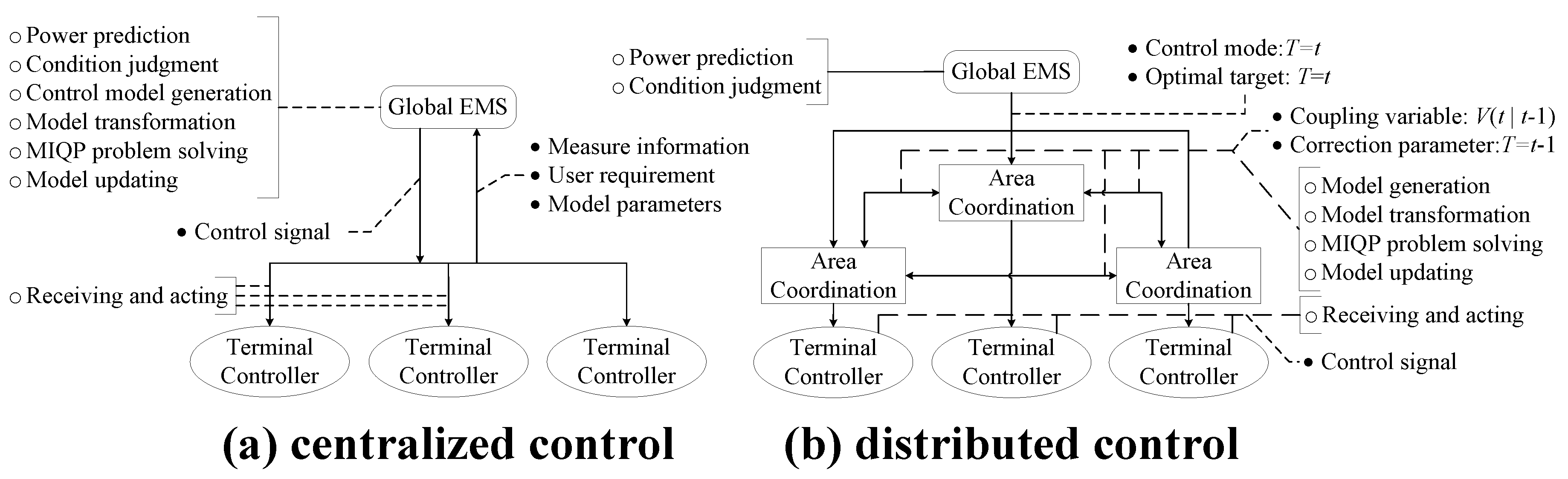
Considering the calculation speed and the existing control system, the second type is more suitable for ADN. Figure 11 shows the differences between distributed control and centralized control in Section 3 of the ADN flexible load when power shortage happens in the feeder. There are three main differences.

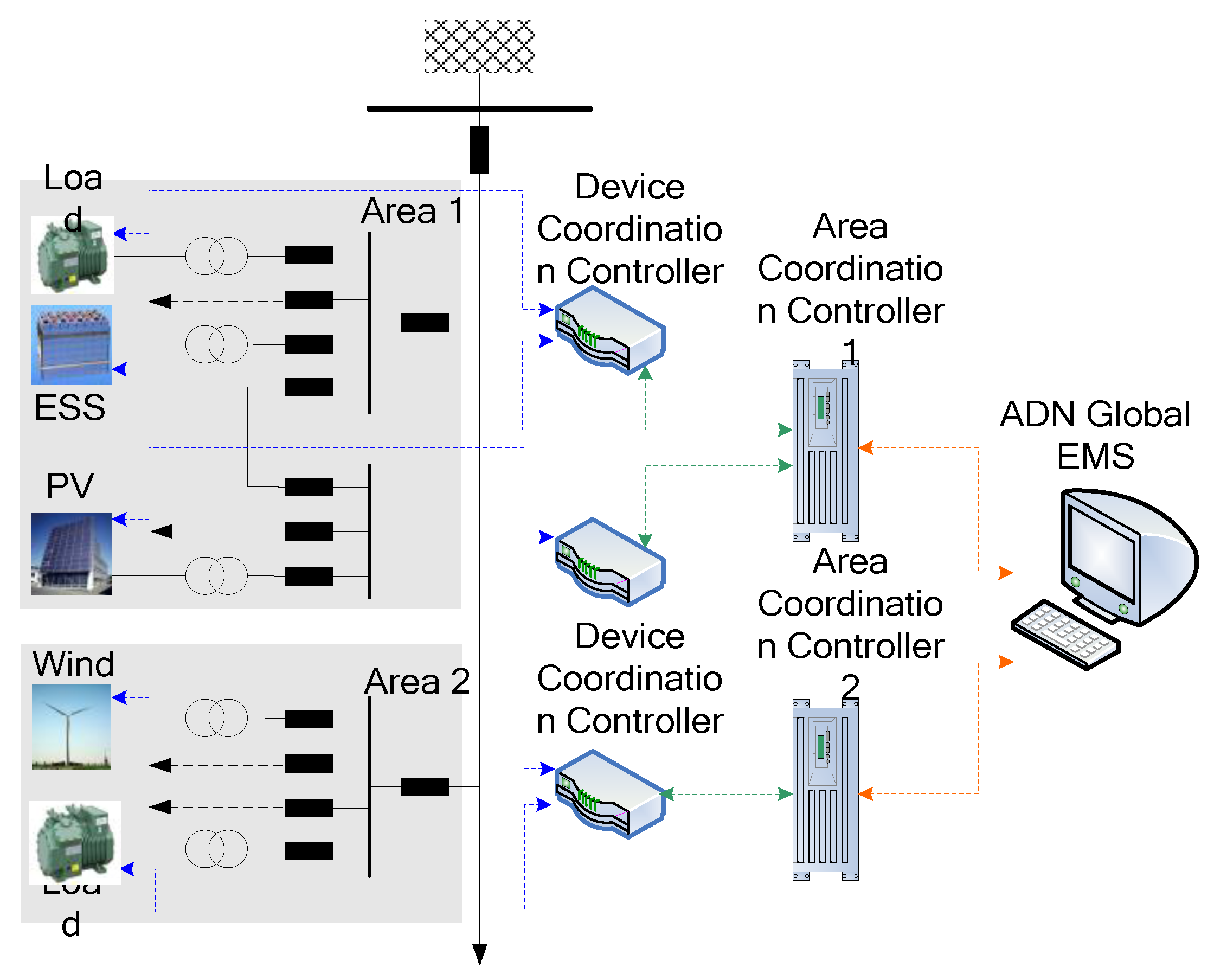
Difference (1): Control structure. The centralized control only has two control levels, global EMS and terminal controller, and all the information is exchanged between these two levels. The distributed mode contains three levels, and the communication not only appears between levels, but also appears between controllers in the same level.

Difference (2): Control task. The hollow circles in Figure 11 indicate the main tasks of each control level. In centralized mode, the global EMS undertakes almost all the modeling and computation but in distributed mode, some tasks are assigned to the area coordination control level.

Difference (3): Control information. The solid circles in Figure 11 show the main information exchanged in the control process. The distributed model adds coupling information transmission of the same level, and because the coupling information is not generated in real time, there is therefore some information of a different time.

Even though, in distributed control, the optimal performance may be lost and the complexity of communication is increased, the control model is simplified significantly and computation time is reduced, also the flexibility of the control is strengthened.

4.2. Distributed Control Model and Method of Flexible Load

When the centralized control solves the optimal model, the coupling relationship between controlled objects exists naturally during the iteration. Only if all the variables including coupling variables satisfy the constraints and optimal purpose, is then the feasible solution acquired. However, the coupling is impossible to automatically appear in the distributed control process, because the sub-problems are separated; additionally, independent control makes it that every controller cannot obtain accurate and real-time state information of the coupled controllers. These two problems are solved by reconstructing the models of Section 3.

(1) Classifying Load Controlled Object

The Load Controlled Object is a flexible loads set, and all the flexible loads of the set are controlled with the same controller. The classification relates to the load type and area, in general, loads of the same type and with similar parameter or the same time step are placed into a category. Let ${(0,1)}^{s\times n}$ express the set of n × n matrices which only consists of elements 0 and 1. Introduce an incidence matrix ${\mathit{A}}_I\in {(0,1)}^{s\times n}$ which defines relation of n loads of s classes in ADN. Only when the matrix’s element A_I(i,j) = 1, i = 1,…,s, j = 1,…,n, the j-th load belongs to the i-th class LCO_i.

(2) Coupling relationship of LCOs

The coupling relationship means that several LCOs affect the optimal target, and this relationship determines if information exchange exists between controllers of the same level. Introduce an incidence vector ${\mathit{A}}_{II-q}\in {(0,1)}^{1\times s}$ which defines the relation between the q-th LCO_q and other s − 1 LCOs. If the q-th LCO_q couples with the p-th LCO_p, the vector’s elements A_II-q(1,p) = 1, p = 1,…,s, p ≠ q, and A_II-q(1,q) = 0.

(3) Coupling variable

In Equation (6), every flexible load contributes to the optimization of total power y(t), and LCOs are the same after the n loads are classified into s LCOs. Hence, the s LCOs has a coupling relation to y(t), that is y(t) = y₁(t) + $\cdots$ + y_q(t) + $\cdots$ + y_s(t).

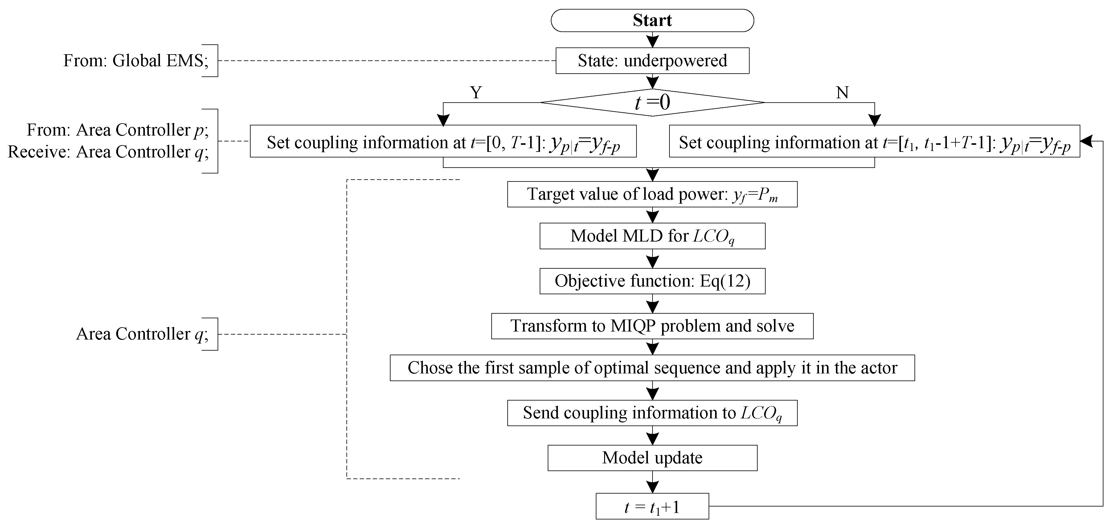
However, each LCO is controlled by the corresponding controller, and the q-th controller Ctrl_q knows the model of q-th LCO_q including the state model (Equation (1)) and the power consumption model (Equation (2)). Moreover, the Ctrl_q does not consider the rest of s − 1 LCOs. Because of this, other controllers such as the p-th controller Ctrl_p must offer power information at time t to the Ctrl_q, that is y(t) = y_1|t(t) + $\cdots$ + y_q|t(t) + $\cdots$ + y_s|t(t), where y_p|t is the knowable coupling variable, p = 1, …, s, and p ≠ q.

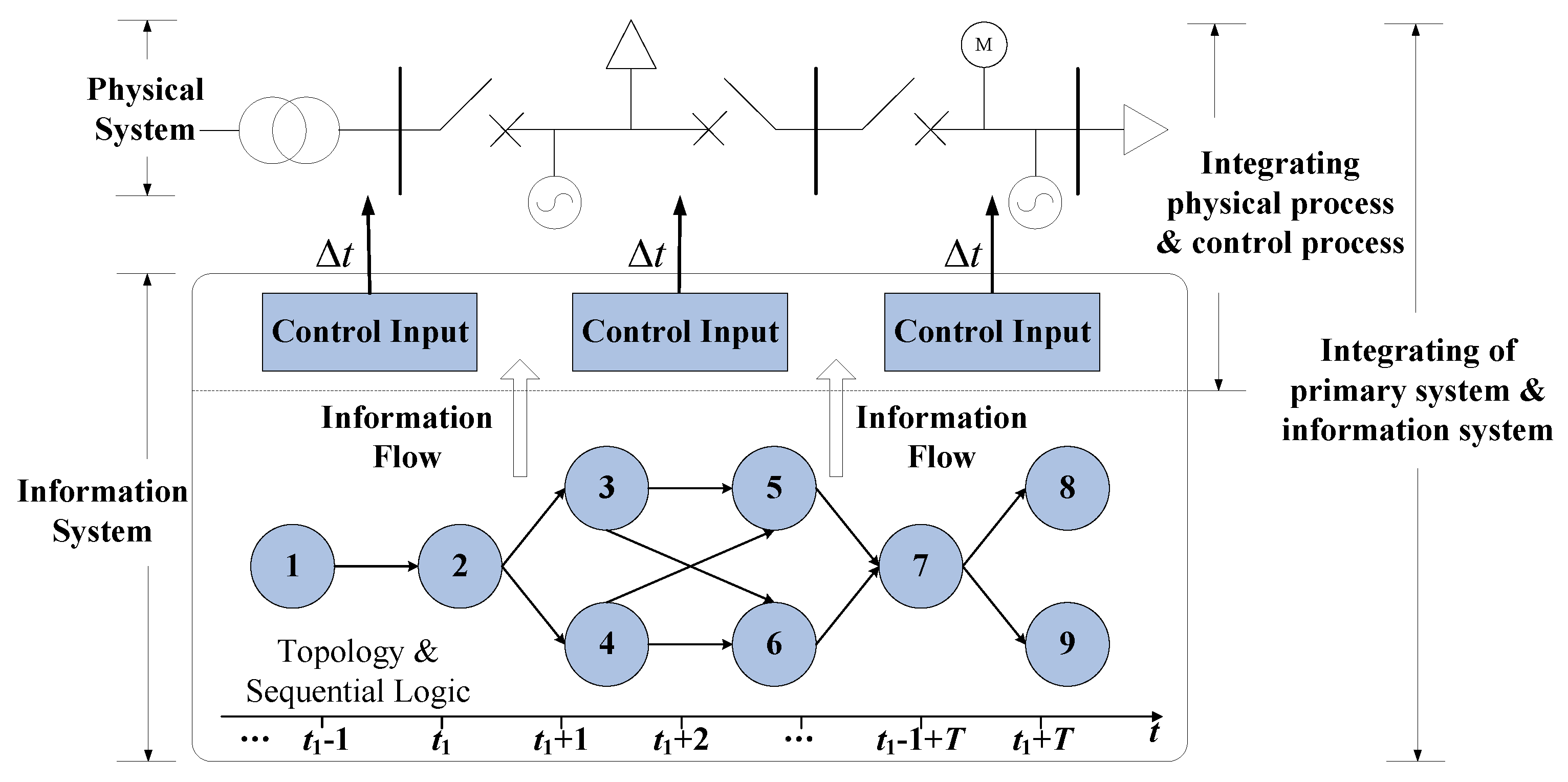
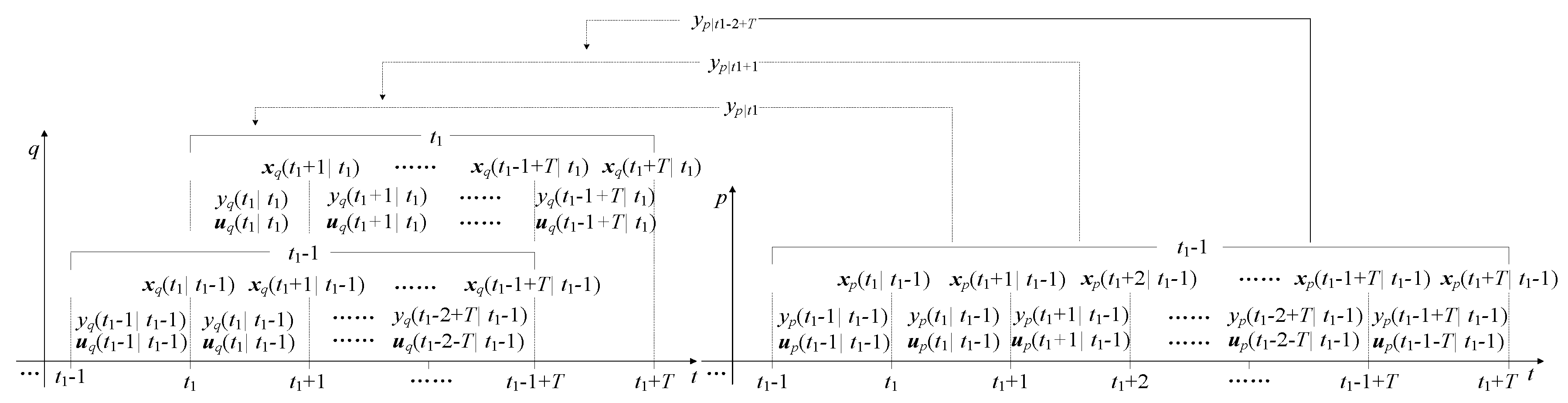
Unfortunately, at time t, due to the same reason of lack of coupling information, y_p|t is unable to be obtained. As shown in Figure 12, the coupling information can be replaced by the predictive control results of [t₁ − 1, t₁ − 1 + T] which are calculated at time t = t₁ − 1, and T is the control period.

According to the principle of receding horizon optimization, when Ctrl_q operates at time t = t − 1, it predicts the LCO_q’s functional index of t = [t₁, t₁ − 1 + T], that is x_q(t₁|t₁ − 1)~x_q(t₁ – 1 + T|t₁ − 1). Then the control input u_q(t₁ − 1|t₁ − 1)~u_q(t₁ − 1 + T − 1|t₁ − 1) and the power y_q(t₁ − 1|t₁ − 1)~y_q(t₁ − 1 + T − 1|t₁ − 1) also can be obtained. Other controllers like Ctrl_p get the power y_p(t₁ − 1|t₁ − 1)~y_p (t₁ − 1 + T − 1|t₁ − 1) too.

With the action of u_q (t₁|t₁ − 1), Ctrl_q moves to time t = t₁, and a new control loop begins. At this time, set y_p|t = y_p(t|t₁ − 1) for every step of t = [t₁, t₁ − 1 + T − 1].

However, for time t = t₁ + T − 1, there is no y_p(t₁ + T − 1|t₁ − 1) that can be assigned to y_p|t1+T-1. Define constants y_f-q and y_f-p, p = 1, …, s, and p ≠ q. y_f-q and y_f-p consist of a power combination of all the LCOs. The power combination corresponds to a kind of load operation mode δ_m and satisfies $y_{f-q}+{\displaystyle \sum _{p=1,p\ne q}^s{y}_{f-p}}=P_m$, where the meaning of δ_m and P_m can be found in 3.3. Let y_p|t1+T-1 = y_f-p, in other words, the unknown coupling variable y_{p|t1+T -1} is set artificially based on P_m. Besides, in the first loop of control, for time t = [0, T − 1], set y_p|t = y_f-p.

(4) Keep the consistency of coupling variables

No matter how the coupling variable gets its value, the Ctrl_p may not follow the y_p|t which has been sent to Ctrl_q. So, there should be some restrictions in optimal function or constraint to keep the actual trajectory of LCO consistent with the coupling variables of the coupled controllers.

In optimal function, during a control period t = [t₁, t₁ + T], minimizing the deviation between y_q(t) and y_q|t, gives Equation (8).

$$\min J_{yq}={\displaystyle \sum _{t=t_1}^{t_1+T-1}\left|\right|y_q(t)-y_{q|t}|{|}_{Q_y}^2}$$

(8)

In control model, add inequality constraints, and make the deviation between y_q(t) and y_q|t of any step during the control period t = [t₁, t₁ + T] not larger than the maximal deviation in the last control period t = [t₁ − 1, t₁ − 1 + T]. That is Equation (9).

$$|y_q(t)-y_{q|t}{|}_{t=[t_1,t_1+T]}\le \max |y_q(t)-y_{q|t}{|}_{t=[t_1-1,t_1-1+T]}$$

(9)

(5) Optimal function

The optimal function of LCO_q includes the functional index deviation J_x, load consumption deviation J_y, and coupling variable deviation J_y.

Like Equation (6), J_x keeps x_q(t) tracing the target x_f-q in the control period t = [t₁, t₁ + T], that is Equation (10).

$$\min J_x={\displaystyle \sum _{t=t_1+1}^{t_1+T}\left|\right|x_q(t)-x_{f-q}|{|}_{Q_x}^2}$$

(10)

J_y contains coupling relationship of LCO_q and LCO_p, and reflects the difference of total consumption and its target. Define matrix $\mathit{Y}\in {ℝ}^{s\times 1}$, $\mathit{Y}={[y_{1|t},y_{2|t},\cdots ,y_{s|t}]}^{\text{'}}$ is the coupling information set of time t which should have been sent by s controllers to each other. Also the load consumption deviation of LCO_q is shown as Equation (11).

$$\min J_y={\displaystyle \sum _{t=t_1}^{t_1+T-1}\left|\right|y_q(t)+{\mathit{A}}_{II-q}\cdot \mathit{Y}-P_m|{|}_{Q_y}^2}$$

(11)

J_yq has been presented in Equation (8). So the optimal function is Equation (12).

$$\min J={\displaystyle \sum _{t=0}^T\left|\right|x_q(t)-x_{f-q}|{|}_{Q_x}^2}+||y_q(t)+{\mathit{A}}_{II-q}\cdot \mathit{Y}-P_m|{|}_{Q_y}^2+||y_q(t)-y_{q|t}|{|}_{Q_y}^2$$

(12)

(6) Control model and method

Model the s LCOs respectively based on 3.2, and MLD models as Equation (5) are acquired. Then add Equations (9) and (12) to each LCO, and the control model is completed.

The optimization problem is that s LCOs are controlled by s controllers on the basis of coupling information to get control inputs. The solution must satisfy Equations (5) and (9), and make Equation (12) optimal.

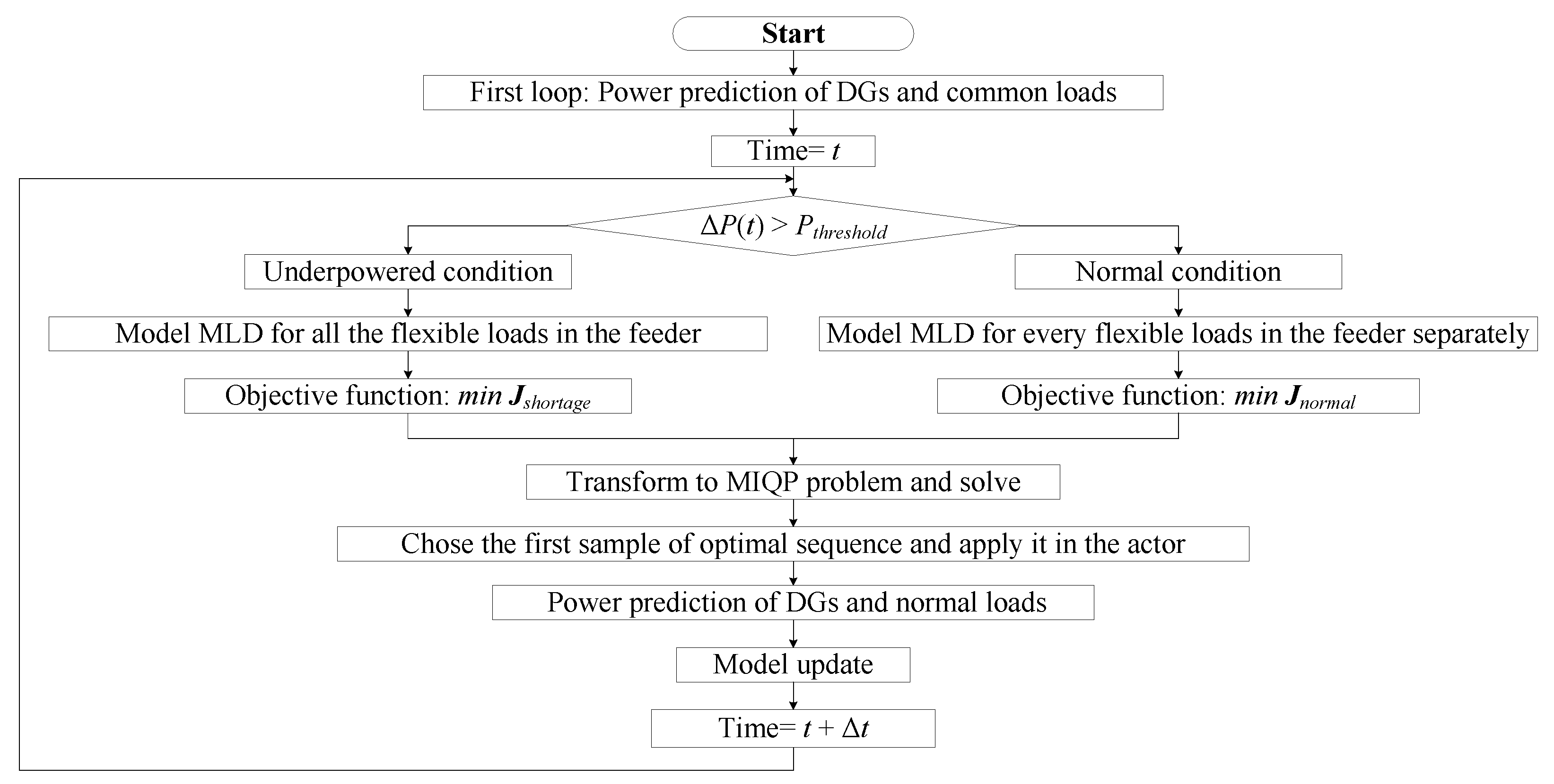
The control procedure is shown in Figure 13. By the prediction of DGs and common loads, the ADN feeder is in the underpowered condition; every controller accepts the coupling information of the other controllers and the power consumption target from the global EMS; all the controllers generate control models of their own LCO and solve them, then act on the first sample of the optimal sequence; all the controllers send coupling information to other controllers and prepare for the next period of control.

4.3. Case Study

The distribution ADN flexible load control model and method of underpowered condition is tested by the case in 3.4.

According to 4.2, the three flexible loads of Load₁, Load₂, Load₃ are classified to three LOCs of LOC₁, LOC₂, LOC₃. Based on Table 3 and Equations (5) and (9), three MLD models of LOCs are built. Set the total power consumption target P_m = 356 kW, then the three optimal functions can be obtained by Equation (12). The models and optimal function are controlled 100 times according to the procedure in Figure 13.

Area coordination controllers are simulated by three IBM Flex System x240 Compute Nodes, and configure another Compute Node to simulate the physical system of the ADN feeder. Each Compute Node contains two Intel Xeon E5-2600 Core6 2.1 GHz processors and 16G memory. An inbuilt Gigabit Switch is used for communication.

Matlab/Simulink is the simulating and computing tool for every Compute Node, and a Socket interface is used for software to communicate with each other. There is also a synchronous program to prevent possible asynchronous problems occurring between different Compute Nodes. So the simulation of ADN feeder including three loads does not begin, only when the feeder has received all the load control inputs from other Compute Nodes.

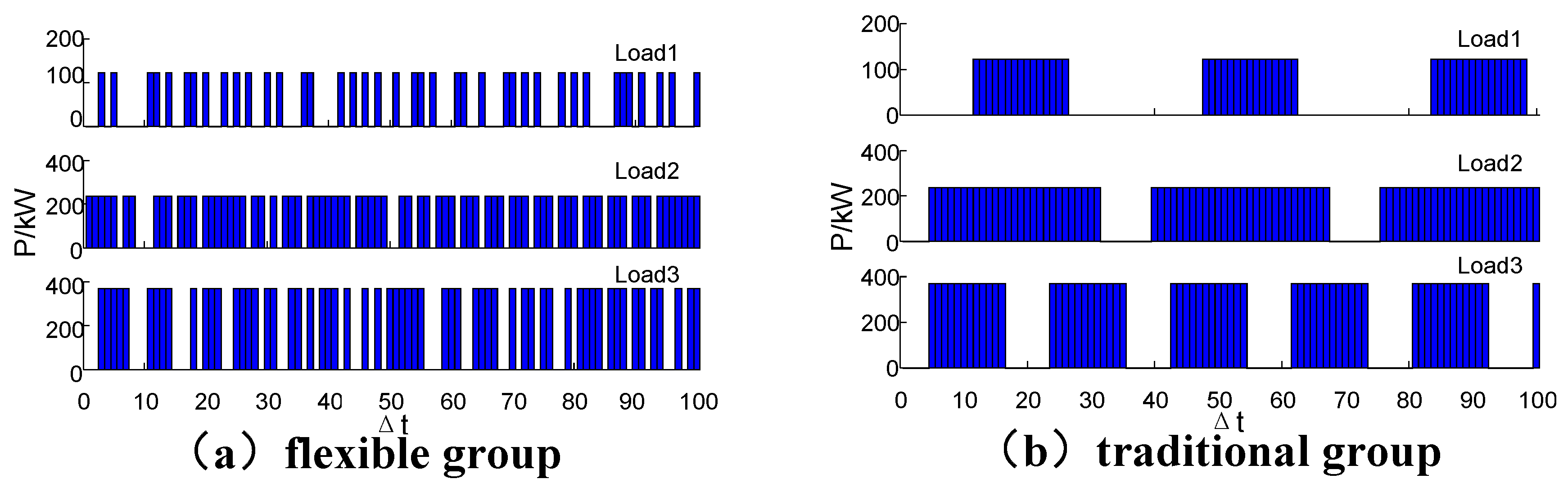
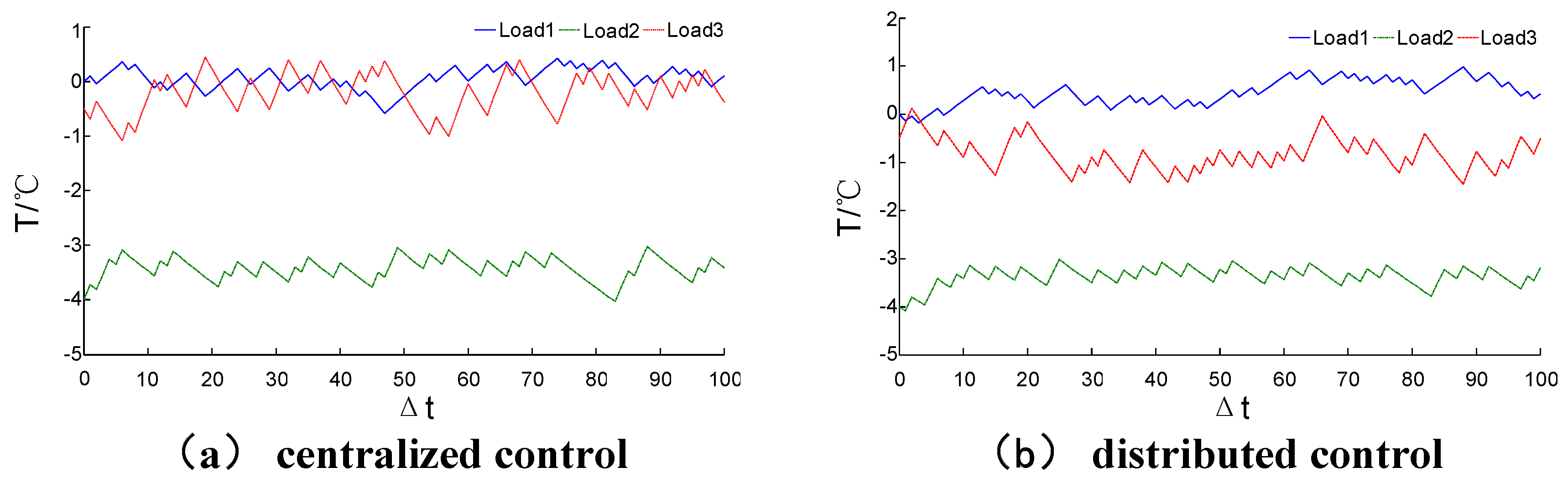
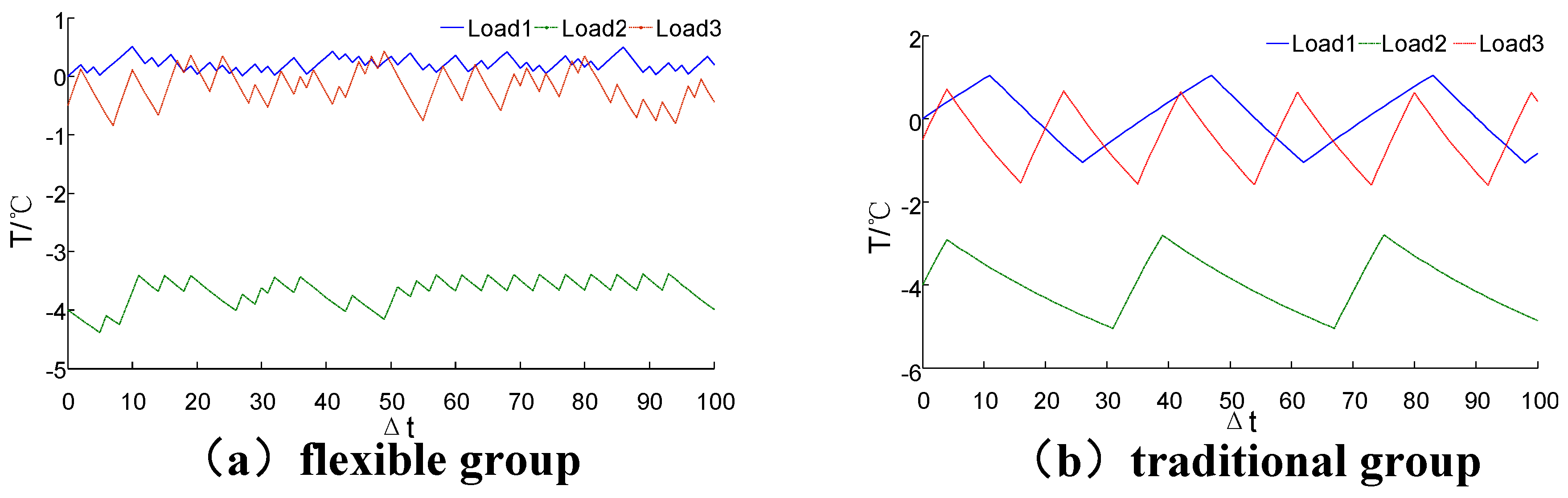
Figure 14 shows the temperature of the distributed and centralized mode in the underpowered condition. The curves of the two modes all locate in the feasible range. The three loads of the distributed mode change their states about 56, 48, and 52 times respectively, and the loads in the centralized mode change only 48, 45, 46 times. The more frequent state switching makes the loads of the distributed mode have a lower fluctuation. Especially the Load₃, it not only operates steadily, but also works at a lower temperature.

This phenomenon is caused by the method difference of how to balance the optimal target of the two modes. Load₃ is the largest load, and the centralized mode considers the optimization from the overall model, so the action of Load₃ should be diminished and the lower loads work more to counteract disturbance. However, in the distributed mode, the controller manages only one load, and does not need to consider other problems.

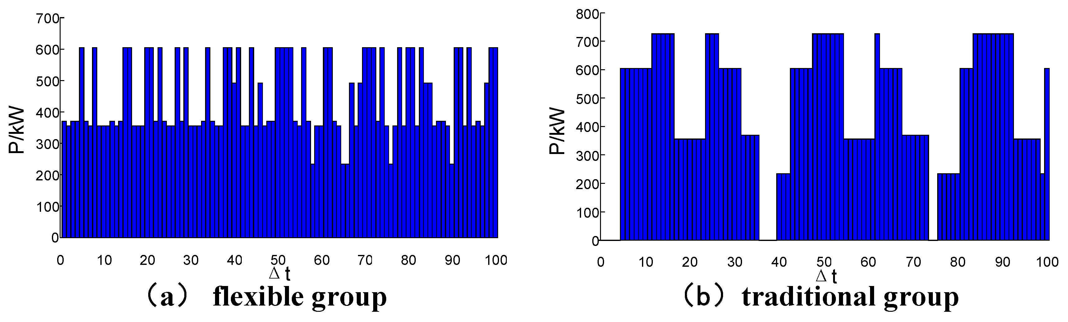
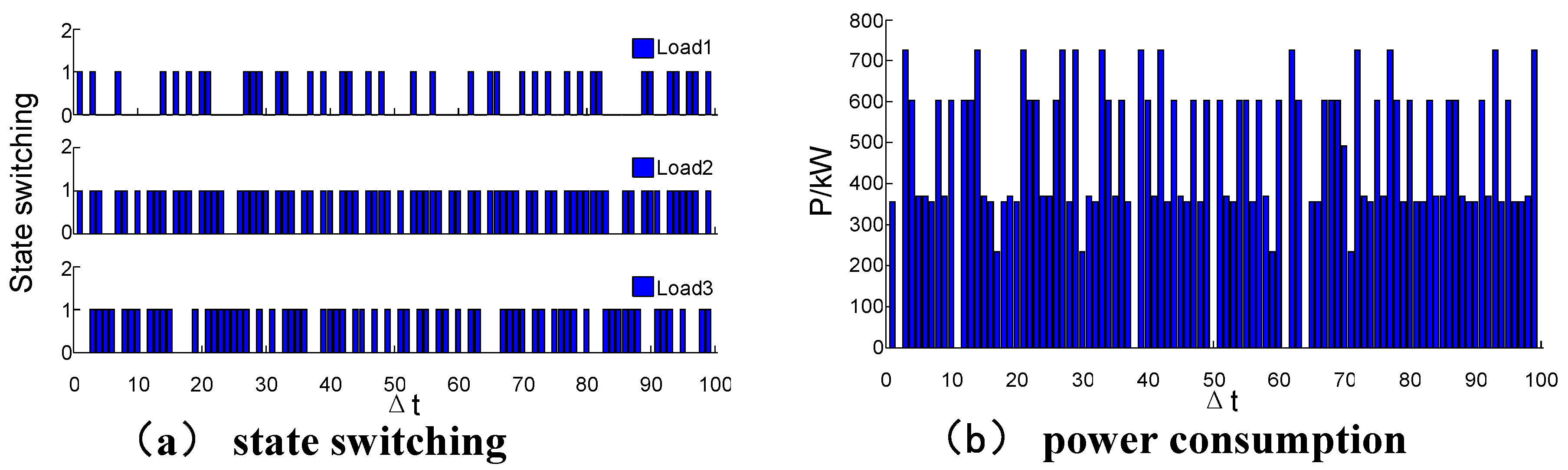
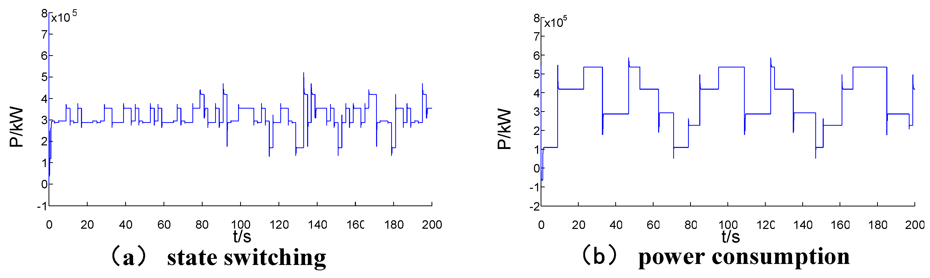
Figure 15 shows the state switching and total power of distributed control. From Figure 15b, the three loads’ total consumption is able to be kept near 356 kW. But compared with Figure 9a, a sharp power change occurs in the distributed mode, and the curve is more unstable. This is caused by inaccurate coupling information between controllers. So, the optimal performance of the distributed mode is worse.

The detailed comparison of total consumption and calculation performance between the two modes is listed in

Table 7. The comparison of centralized and distributed control.

Control	Power Consumption	Max Load Difference	RMS	Target Deviation	Computing Time
Centralized	24.81 kW·h	370 kW	462.81 kW	30%	1.847 s
Distributed	25.17 kW·h	726 kW	486.98 kW	37%	1.053 s

. Though there is a loss of optimal performance, the speed of distributed control is promoted.

5. Conclusions

The characteristics of discrete and logical of the control system determine that in order to realize integrated analyzing and control of Power CPS, the first thing is to build a Hybrid System model which is able to describe the continuous dynamic process and discrete process for the primary system of the power grid.

This paper applies the MLD method to build a Hybrid System based Power CPS control model for ADN flexible load control. Combining with the ADN feeder power control, a flexible load control strategy is designed for normal and underpowered conditions of ADN feeder. To solve the problems of centralized control mode when the feeder is in the underpowered condition, a model and method of distributed control for flexible load is proposed.

From the study case, it can be concluded that compared with the traditional load control, the proposed flexible load control contains two advantages: (1) With the help of the hybrid model the predictability of the control is better, by which the flexible loads’ operation constraints are satisfied strictly when the traditional loads violate the limit; (2) The hybrid model has the ability to combine the discrete process into the optimal control of continuous variables, in that the ADN flexible load state switching can be optimized to meet continuous variables, so that ADN flexible load state switching can be optimized to meet consumption demand. In the case study simulation of this paper, the flexible load power consumption is lower, and the most load’s energy conservation reaches 11% of the traditional load; when the coordinates with DGs in the ADN, flexible load power consumption can be sustained near a target value and the deviation of RMS is 30% which is lower than 46% of the traditional load control.

Simulations of centralized and distributed control models of flexible load show that both of them have their advantages and disadvantages. The centralized control has higher efficiency and the target deviation is 7% lower than the distributed control in the study case. However, the distributed control is suitable for some complex situations, and computes faster (0.794 s in study case) than the centralized mode. Besides, the distributed control makes full use of the ADN control system, and has some practical value.

In conclusion, the Hybrid System based model proposed in this paper combines continuous dynamic, discrete state and even complex logical description in a unified expression, therefore physical process, control process and information flow is able to be described by mathematics directly. According to the model, the control method optimized continuous variables and state switching together in a control step. The ADN flexible load control is an example to illustrate the “integrating physical process and the control process” of the “Control Model”, and the characteristics of the information system will be considered in the future to show the “integration of the primary and information systems”.