Principal Mismatch Patterns Across a Simplified Highly Renewable European Electricity Network


1
Department of Physics and Astronomy, Aarhus University, Ny Munkegade 120, 8000 Aarhus C, Denmark
2
DONG Energy A/S, Teknikerbyen 25, 2830 Virum, Denmark
3
Department of Engineering, Aarhus University, Inge Lehmanns Gade 10, 8000 Aarhus C, Denmark
*
Author to whom correspondence should be addressed.
†
These authors contributed equally to this work.
Energies 2017, 10(12), 1934; https://doi.org/10.3390/en10121934
Submission received: 19 September 2017
/
Revised: 17 November 2017
/
Accepted: 20 November 2017
/
Published: 23 November 2017
(This article belongs to the Section F: Electrical Engineering)
Abstract
:Due to its spatio-temporal variability, the mismatch between the weather and demand patterns challenges the design of highly renewable energy systems. A principal component analysis is applied to a simplified networked European electricity system with a high share of wind and solar power generation. It reveals a small number of important mismatch patterns, which explain most of the system’s required backup and transmission infrastructure. Whereas the first principal component is already able to reproduce most of the temporal mismatch variability for a solar dominated system, a few more principal components are needed for a wind dominated system. Due to its monopole structure the first principal component causes most of the system’s backup infrastructure. The next few principal components have a dipole structure and dominate the transmission infrastructure of the renewable electricity network.
1. Introduction
Weather is the driving force in a highly renewable energy system. The planning for such systems requires an in-depth understanding of the variable mismatch between weather and demand patterns on multiple time and length scales [1,2]. The spectrum of prominent temporal fluctuations of wind and solar power generation ranges from seconds to years [3,4,5,6], and impacts the design and operation of power systems [7,8,9,10,11,12,13]. The planning of large-scale energy systems is also affected by the spatial variability of the weather. Wind power generation is correlated up to a length scale of about 500 km [4,14,15,16]. Approaches based on spatial correlations, such as the optimal portfolio theory [17,18,19] and the copula method [20], are used for systemic resource assessments of renewables and for analysis of national and continental power grids.
Weather-driven network modelling represents a more direct approach to obtain estimates on the required backup infrastructure of highly renewable large-scale energy systems [21,22,23,24,25,26,27,28,29]. Weather data covering multiple years are converted into prospective wind and solar power generation with good spatial and temporal resolution [21,22,30,31,32], and are then used as the driving force in networked electricty system models. This modelling approach has produced estimates on the required amount of conventional backup power plants, transmission lines and storage [22,23,24,25,26,27,28,33,34,35,36,37,38]. Also the optimization of levelized system cost of energy has been addressed and has led to new design concepts, such as the optimal heterogeneity and the benefit of cooperation [29,39,40,41,42].
Weather-driven network modelling takes the high-dimensional weather and demand data “as is”, and “computes everything away” by brute force. The resulting infrastructure estimates might not depend on all of the mismatch data. To a large part they might only depend on a few dominant mismatch patterns. This is the central topic of this paper. The central question is: what are the dominant spatio-temporal mismatch patterns between the renewable power generation and the load which determine most of the required infrastructure of a highly renewable European electricity system? The central method to apply is a principal component analysis (PCA) [43].
Spatio-temporal pattern analyses, such as PCA, are well known in meteorology. In [44] a PCA has been used to extract the main pattern of variability of wind power generation in Germany, and a wind power forecasting model has been implemented with this approach. In [45] a PCA has been applied to distributed wind power data from Irish wind farms and used as a multivariate dimension reduction scheme to obtain potential wind power production costing simulation efficiency gains, when compared to exhaustive multi-year time series load flow investigations.
This paper has the following structure: Section 2 describes a simplified weather-driven European electricity system with a high share of wind and solar power generation, including several of its infrastructure measures. A short description of the PCA is also given. Section 3 presents the results on the dominating principal mismatch components and their dependence on the share between wind and solar power generation. Section 4 reveals how the principal components contribute to the backup and transmission infrastructure estimates. A conclusion and outlook is given in Section 5.
2. Modelling and Methods
2.1. Modelling of a Simplified Highly Renewable European Electricity Network
We follow the simplified approach introduced by [22,23,26,46] to model a highly renewable European electricity system. The key variable is the mismatch
between the renewable power generation and the load at time t for country n in Europe. With a flipped sign the mismatch is often also denoted as the residual load. The renewable power generation
is composed of wind and solar power generation only; other forms of renewable power generation are discarded. The average wind and solar power generation amount to
and define two design parameters, the renewable penetration with respect to the average load and the renewable mix between the average wind and solar power generation.
Penetration parameters around one describe highly renewable electricity networks. We choose for all countries. This setting describes a self-sustainable renewable limit, where in each country the average renewable power generation is equal to the average load. For simplicity, the renewable mixing parameter is also chosen to be the same for all countries. These homogeneous layouts have been first discussed in [22,23,33]. Recently also heterogeneous layouts with differing renewable penetration and mixing parameters between the countries have been investigated [41].
The hourly time series , , for the country-aggregated wind power generation, solar power generation and load are taken from Refs. [22,23], where wind velocity and solar irradiation data from the private weather service provider WEPROG (Böblingen, Germany) [47] with hourly temporal resolution and spatial resolution have been convoluted with country specific capacity layouts adapted from EuroStat; see also Refs. [30,31,32] for related approaches. The data cover the years 2000–2007 for all European countries. It is assumed that this data is also statistically representative for future years. The hourly load time series have been detrended such that the annual consumption of each year matches that of 2007. A possible dependence of the load time series on efficiency improvements, de-industrialisation, electrification of heat and transport, and climate conditions [48,49] has not been considered.
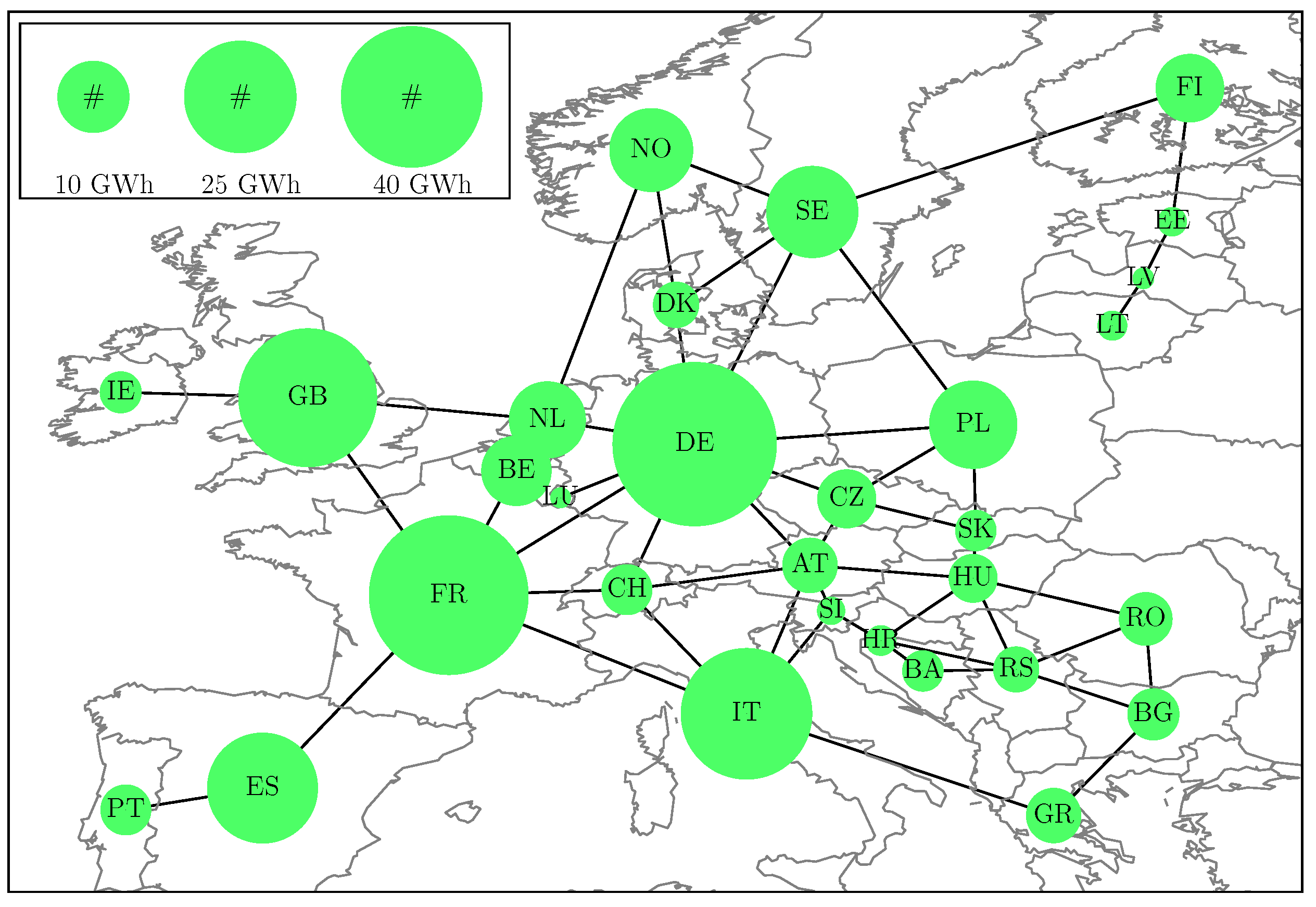
The average loads are illustrated in Figure 1. Note that the average loads set the absolute scales for the simplified modelling of a highly renewable European electricity network. If future values should increase or decrease, but such that the relative load strengths between the countries remain unchanged, then the infrastructure measures (to be discussed in the next subsection) will linearly scale with changes of the average loads. Figure 1 also shows the interconnecting transmission lines between the countries.
With the chosen setting the average mismatch is . However, most of the times the actual mismatch is non-zero. It is either positive when the wind and the solar radiation are strong, or negative when they are weak. The overall electricity system needs to respond to these mismatch fluctuations. In simplified form, the response can be written as
The nodal balancing determines the backup power generation and the curtailment,
The nodal injection into the networked system describes the exports () and imports (), and has to fulfill . The nodal injections determine the power flows
on the interconnecting transmission lines l between the countries. The linear relationship between the flows and the injections is described by the matrix of the power transfer distribution factors [50], which are constructed from the Moore-Penrose pseudo inverse of the graph Laplacian of the underlying electricity network topology [51]. In principle, more terms can be added to the right hand side of the nodal response Equation (4), such as for example, storage, but for the present purpose we leave this equation as is.
The response (4) allows for various schemes which divide differently between balancing and injection. For sure the simplest scheme is for all nodes and all times, but has the disadvantage that each node has to fully balance its mismatch alone without the benefits of importing and exporting across the network. Market schemes could be used to settle the dispatch between renewable and backup power generation, but due to the simplicity of the current modelling approach this would be, such as, shooting pigeons with canons. We adopt the simple scheme of synchronised nodal balancing
which has been proposed in [46]. It distributes the actual overall mismatch onto all nodes in proportion to their average load. In view of the upcoming expression (11), this scheme also distributes the required overall backup capacities onto the nodes in the same way.
2.2. Infrastructure Measures
If the mismatch (1) was zero for all times and all countries, the infrastructure response (4) would simply be zero, and no backup power plants and no transmission lines would be required. Of course, this is almost surely never the case. This sets the stage for the mismatch variance to become a first infrastructure measure:
The components of the mismatch/balancing/injection vectors are given by the nodal mismatches /balancings /injections . The second step, which uses (4), relates the mismatch variance to the variances of the balancings and the injections as well as to their covariance. This emphasises that a small mismatch variance would require a small backup and transmission infrastructure, and a large variance would lead to a bigger infrastructure.
The mismatch variance (8) represents only a rough infrastructure measure. More specific measures are given by the total backup energy, the total backup capacities and the total transmission capacities:
The backup capacities and the transmission capacities are defined via the quantiles of the time-sampled distributions and , respectively. N and L represent the number of nodes and links illustrated in Figure 1. The link length is denoted as and is approximated as the distance between country capitals.
2.3. Principal Component Analysis
We follow the notation of Ref. [43] and sketch the main steps of the Principal Component Analysis (PCA). The mismatch vector is rescaled to
where the normalisation c is chosen such that . This turns into a function of the mixing parameter . Note that the new variable is usually defined with the centred mismatch , but with our choice for the renewable penetration parameter the average mismatch is zero. The normalised mismatch vector (13) is represented in an N-dimensional coordinate system, where the axes with unit vectors correspond to the countries.
The PCA changes this coordinate system by rotation. The normalised mismatch vector
is then expressed in terms of the rotated unit vectors . Those are determined from the diagonalisation
of the covariance matrix
Since the covariance matrix is real and symmetric, the eigenvectors are orthonormal, i.e., , and all eigenvalues are real and positive. Furthermore, because of the normalisation introduced in Equation (13).
The temporal amplitudes have the properties and . The total variance (8) of the mismatch can now be written as
Given the ordering , the last equation reveals that the first eigenvector with the largest eigenvalue contributes most to the total variance. This implies that the mismatch can be approximated by a truncation to the first K eigenvectors with the largest eigenvalues:
This approximation explains the naming of the PCA: the eigenvectors with the K largest eigenvalues are called the principal components and carry most of the overall variance. Typically, the truncation parameter K is determined by the requirement , such that the K principal components carry about 95% of the overall mismatch variance. The K principal components represent the main degrees of freedom of the driving force resulting from the mismatch between the weather and load patterns, and cause most of the required backup and transmission infrastructure.
3. Results: Principal Mismatch Components
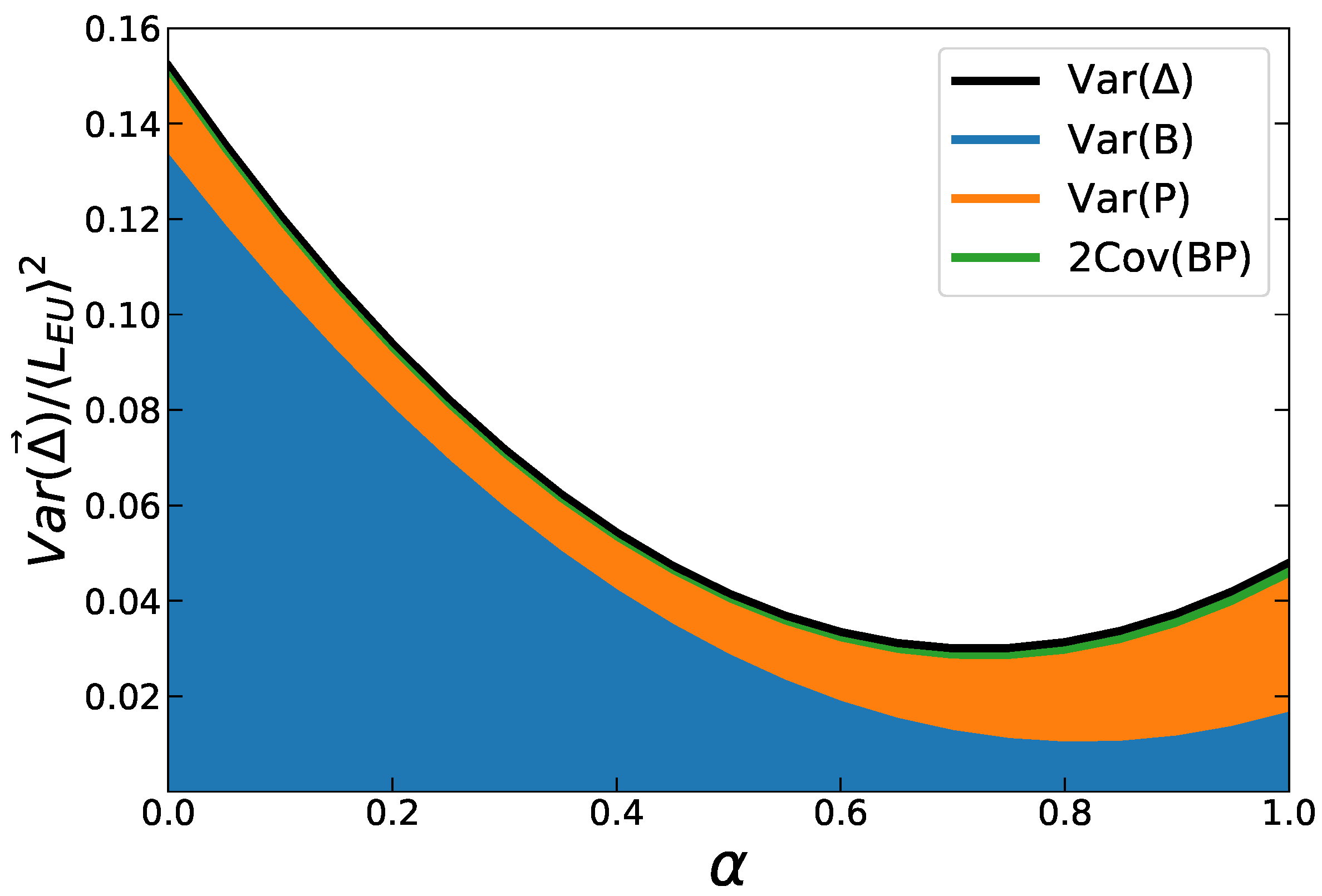
The dependence of the mismatch variance (8) on the renewable mix is shown as the thick black curve in Figure 2. The renewable penetration has been set to for all European countries. The variance takes a minimum at . It is slightly larger in the wind-only limit and significantly larger in the solar-only limit . This can be seen as a rough indication that the response infrastructure becomes smallest at intermediate renewable mixes, and agrees nicely with the results on the other infrastructure measures (10)–(12) obtained in [23,46].
The eigenvalues resulting from the Principal Component Analysis reveal the dominant contributions explaining most of the mismatch variance. They are shown in Figure 3, again as a function of the renewable mix. In the solar-only limit the largest eigenvalue is . The three largest eigenvalues add up to 0.96, explaining 96% of the mismatch variance. Not much changes for renewable mixes up to about . After this the largest eigenvalue decreases continuously, until it reaches a value at . It roughly remains at this value for even larger renewable mixes. As the first eigenvalue decreases, the next eigenvalues increase. At the first six eigenvalues add up to 0.94, explaining then 94% of the mismatch variance.
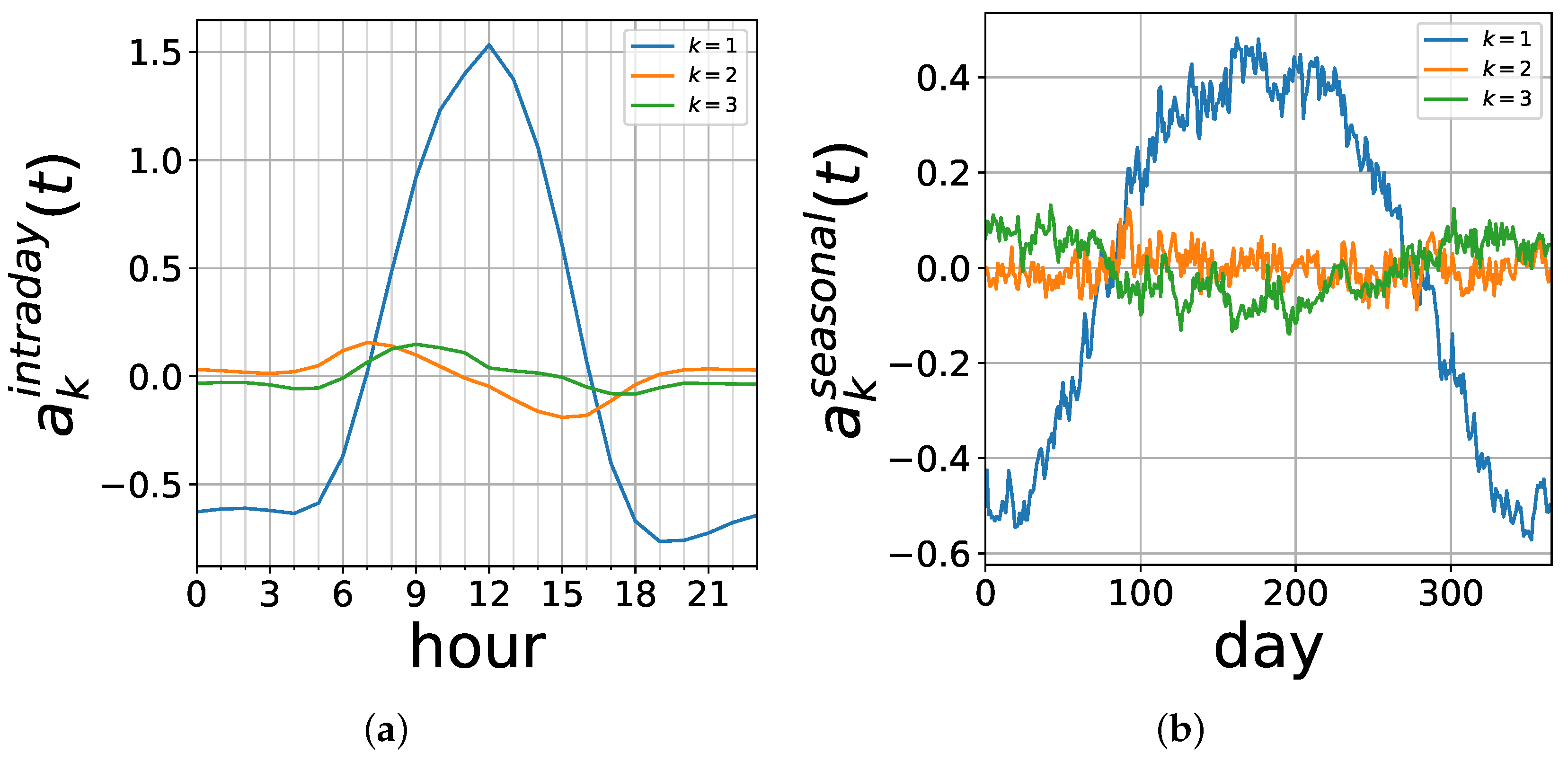
A threshold like for the first eigenvalues is often used as a criterium to define the number K of principal components. Together they explain 95% of the mismatch variance. For this number is equal to . The corresponding eigenvectors are shown in Figure 4. The first principal component is a kind of monopole. All countries either have a positive mismatch together or a negative mismatch. Of course, this is easy to understand. Either the sun is shining for all countries during daytime, or it is dark for all countries during nighttime. The second principal component looks like a dipole in East-West direction. It is a consequence of morning sunrise in the East and of evening sunset in the West. These interpretations are clearly supported by the intraday amplitude profiles , which are shown in Figure 5a.
In addition, the third principal component has a dipole structure, but with a North-South orientation. This is mostly a consequence of its seasonal amplitude profile , which is shown in Figure 5b. Figure 5b also reveals that the first principal component has a very pronounced seasonal amplitude profile, whereas no clear seasonal dependence is observed for the amplitude of the second principal component.
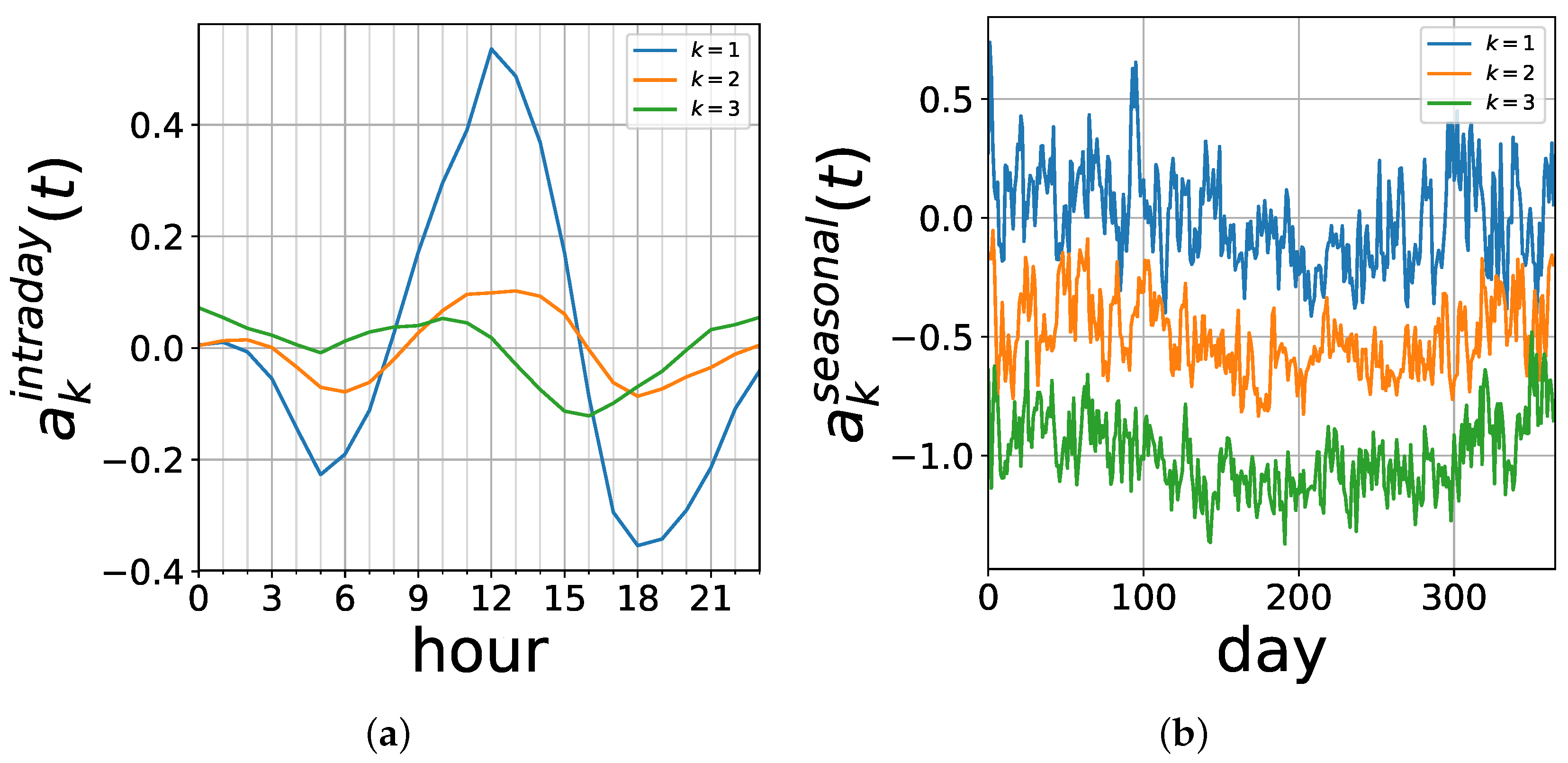
Figure 6 depicts the principal components for the renewable mix , which together explain 94% of the mismatch variance. The first principal component again looks like a monopole. Roughly it means the wind power generation is above the load for all countries at the same time, or vice versa. Its eigenvalue is smaller than for the case, and also its structure appears to be slightly different. The other five principal components represent different orthogonal spatial mismatch patterns. The second and third one look again like dipoles. The fourth to sixth principle components have a more complicated spatial structure.
Again it is interesting to investigate the time dependence of their amplitudes . The intraday and seasonal profiles are shown in Figure 7 for the first three principal components. The intraday amplitude profile of the first principal component has two minima, one during the morning and another one during the evening hours. They are explained by the morning and evening peaks of the load. The maximum at noon traces back to the midday solar power generation, which on average still contributes 20% to the overall renewable power generation due to the setting for the renewable mix. The amplitude shows a similar intraday profile, although much weaker than for the amplitude. The seasonal amplitude profiles of the first three principal components all follow the same trend and are correlated to the seasonal wind power generation, which is larger in winter and smaller in summer. The fluctuations on the synoptic time scale of the order of a few days are also clearly visible.
4. Discussion: Contribution of Principal Mismatch Patterns to the Balancing and Transmission Infrastructures
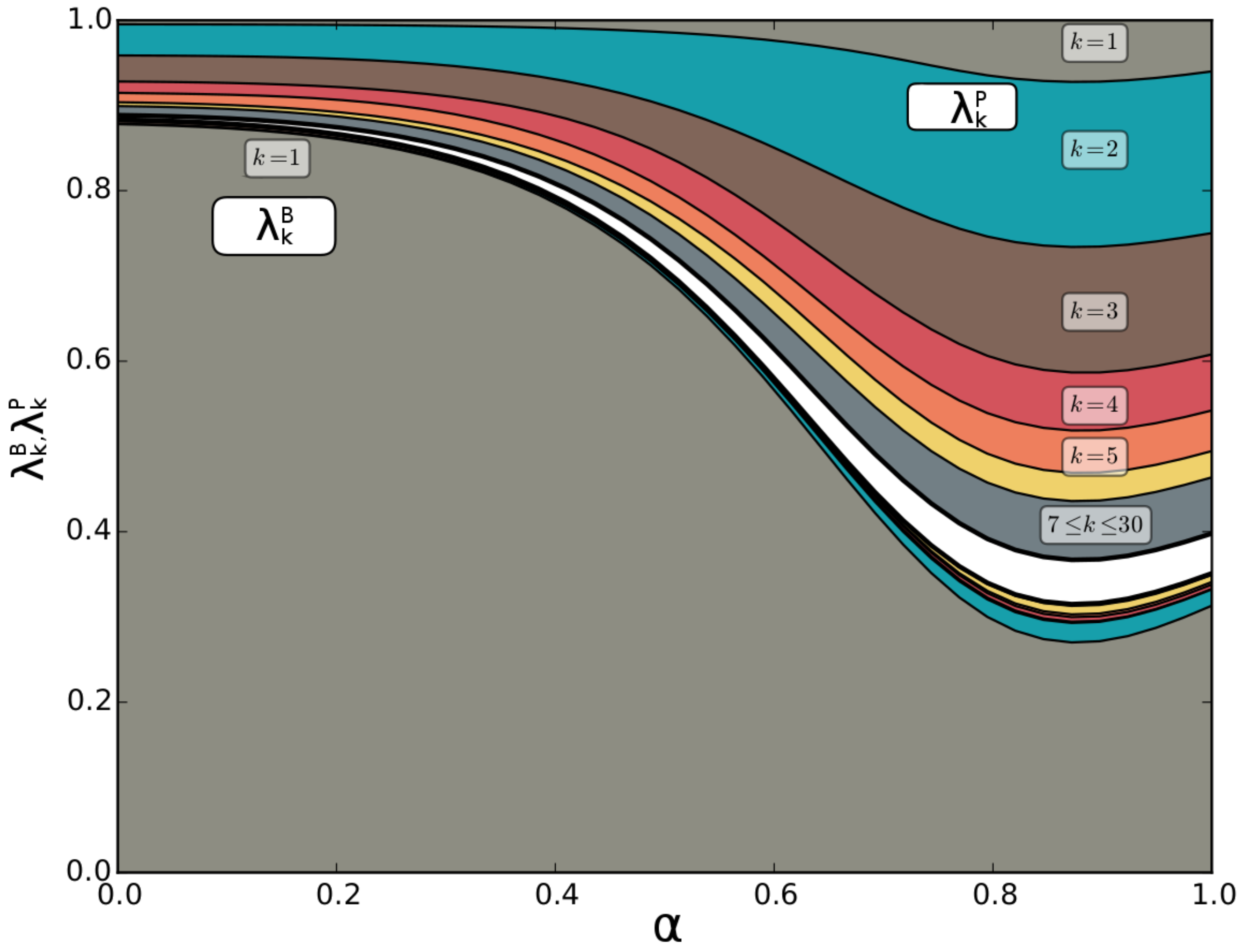
According to Equation (9) the mismatch variance splits into the balancing variance, the injection variance and the covariance between balancing and injection. The three contributions are also shown in Figure 2. For a small renewable mix the balancing variance dominates, but for large mixes the injection variance becomes bigger. The covariance between the balancing and the injection response remains very small, independent of the wind/solar mix. It is now interesting to investigate how the different principal mismatch components contribute to the balancing and injection variances.
The PCA eigenvalues can be split into the same three contributions. Making use of the results of Section 2.3 and of the response Equation (4), the PCA amplitudes can be written as . In the last step the abbreviations and have been introduced. This allows to write the eigenvalues as
This decomposition reveals how much a principal component is contributing to the balancing and injection variances.
Figure 8 illustrates this decomposition. The balancing eigenvalues are plotted from the bottom, and the injection eigenvalues are arranged from the top. The narrow white stripe in the middle represents the sum and is not specified further into the different k contributions. The first principal component dominates the balancing variance, independent of the renewable mix. This is because of its monopole-like structure. The other components do not contribute much, and only with a small margin for renewable mixes close to one. On the contrary, the first prinicipal component does not contribute much to the injection variance. Here the largest contributions come from the second and third principal component. Again this is intuitive due to their dipole character. For large renewable mixes also the next three principal components contribute to the injection variance to a larger extend.
These results are also documented in Table 1 for the specific choice of the renewable mix. The mismatch has been truncated according to (18). The full () balancing variance is fully reproduced with the principal components. A severe truncation to is still able to reproduce 88% of the full balancing variance, emphasising again the dominant role of the first principal component for the mismatch-induced balancing. For the injection variance a different finding is observed. The first principal component alone, reflected by the truncation, does play only a small role. The second and third principal component contribute the most, but are not able to explain all of the variance. The first principal components taken together are able to explain 89% of the full () injection variance. Apparently, higher-order components with still play a small role.
Table 1 lists also the other, more realistic infrastructure measures introduced in Section 2.2. The balancing energy and the backup capacity are related to the balancing variance . Again, the first principal component dominates in both cases, and the truncation is able to explain 99% of the full results. The flow variance
and the transmission capacity are related to the injection variance . The findings for (20) are very similar to those for the injection variance. The truncation is able to explain 84% of the full flow variance. For the transmission capacity (12) the first principal component appears to play a slightly larger role. The truncation is able to explain 82% of the full result.
5. Conclusions and Outlook
Principal Component Analysis has been applied to a simplified highly renewable European electricity system to learn about the most important mismatch patterns between the weather-driven renewable power generation and the load. For a solar dominated system three principal components are enough to explain most of the mismatch variance across the continent. For a wind dominated system six principal components are needed. The spatial structure of the first principal mismatch component resembles that of a monopole, and the respective temporal amplitude dynamics reveals strong fluctuations on the diurnal and seasonal time scales. It determines most of the required backup energy and backup capacity of the overall system. The second and third principal components have a dipole-like spatial structure; their temporal amplitude dynamics is dominated by diurnal, synoptic and seasonal time scales. Together with the fourth to sixth principal components they cause most of the required transmission infrastructure. These results demonstrate that the required backup and transmission infrastructure of a highly renewable European electricity system are to a large degree caused by only a small number of most important mismatch patterns between the weather-driven renewable power generation and the load.
The model used for a highly renewable European electricity system had been quite simple. In particular, its spatial resolution has been scaled to country sizes. As a consequence, the covariance matrix underlying the Principal Component Analysis is dominated by the larger countries like Germany, France, United Kingdom, Spain and Italy. It is interesting to observe that in the most important principal components the smaller countries appear to be grouped into blocks, such as Scandinavia and East Europe. Nevertheless, the next step to take will be to apply the Principal Component Analysis to larger, fine-grained continental electricity networks, with the additional inclusion of hydro power and storage. In view of the higher dimensionality, the resulting number of principal components is certainly going to increase, but per se it is not clear by how much and how the fine-grained spatial structure of the principal patterns is going to look like. In this respect it will also make sense to investigate related data-reduction approaches like Independent Component Analysis and Dynamic Mode Decomposition [52].
Another future step to take will be the stochastic modelling of the amplitude times series related to the principal components. This can be used for the forecasting of power mismatches, and it will also allow to estimate the additional infrastructure due to the operational forcast uncertainties. An example would be line congestion in transmission systems under uncertainty [53]. Another playground for the application of the Principal Component Analysis could be the impact of climate change on the design of future energy systems, in particular smart energy systems including all cross-sector couplings [54].
Supplementary Files
Supplementary File 1Acknowledgments
The authors thank Smail Kozarcanin, Fabian Hofmann, Jonas Hörsch and Tom Brown for helpful discussions. Kun Zhu and Martin Greiner are fully/partially funded by the RE-INVEST project (Renewable Energy Investment Strategies—A two-dimensional interconnectivity approach), which is supported by Innovation Fund Denmark (6154-00022B). The responsibility for the contents lies solely with the authors.
Author Contributions
Mads Raunbak, Timo Zeyer and Kun Zhu performed the model simulations and analysis, and produced the figures; Martin Greiner wrote the paper.
Conflicts of Interest
The authors declare no conflict of interest.
Abbreviations
The following abbreviations are used in this manuscript:
| PCA | Principal Component Analysis |
References
- Graabak, I.; Korpås, M. Variability characteristics of European wind and solar power resources—A review. Energies 2016, 9, 449. [Google Scholar] [CrossRef]
- Engeland, K.; Borga, M.; Creutin, J.D.; François, B.; Ramos, M.H.; Vidal, J.P. Space-time variability of climate variables and intermittent renewable electricity production—A review. Renew. Sustain. Energy Rev. 2017, 79, 600–617. [Google Scholar] [CrossRef]
- Holttinen, H. Wind power variations in the Nordic countries. Wind Energy 2005, 8, 173–195. [Google Scholar] [CrossRef]
- Apt, J. The spectrum of power from wind turbines. J. Power Sources 2007, 169, 369–374. [Google Scholar] [CrossRef]
- Milan, P.; Wächter, M.; Peinke, J. Turbulent character of wind energy. Phys. Rev. Lett. 2013, 110, 138701. [Google Scholar] [CrossRef] [PubMed]
- Grams, C.; Beerli, R.; Pfenninger, S.; Staffell, I.; Wernli, H. Balancing Europe’s wind-power output through spatial deployment informed by weather regimes. Nat. Clim. Chang. 2017, 7, 557–562. [Google Scholar] [CrossRef] [PubMed]
- Holttinen, H.; Milligan, M.; Kirby, B.; Acker, T.; Neimane, V.; Molinski, T. Using standard deviation as a measure of increased operational reserve requirement for wind power. Wind Energy 2008, 32, 355–378. [Google Scholar] [CrossRef]
- Holttinen, H.; Meibom, P.; Orths, B.; Lange, M.; O’Malley, M.; Tande, J.O.L.; Estanquerio, A.; Gomez, E.; Söder, L.; Strbac, G.; et al. Impacts of large amounts of wind power on design and operation of power systems—Results of IEA collaboration. Wind Energy 2011, 14, 179–192. [Google Scholar] [CrossRef]
- Tarroja, B.; Mueller, F.; Eichman, J.D.; Samuelsen, S. Metrics for evaluating the impacts of intermittent renewable generation on utility load-balancing. Energy 2012, 42, 546–562. [Google Scholar] [CrossRef]
- Lannoye, E.; Flynn, D.; O’Malley, M. Evaluation of power system flexibility. IEEE Trans. Power Syst. 2012, 27, 922–931. [Google Scholar] [CrossRef]
- Huber, M.; Dimkova, D.; Hamacher, T. Integration of wind and solar power in Europe: Assessment of flexibility requirements. Energy 2014, 69, 236–246. [Google Scholar] [CrossRef]
- Ulbig, A.; Andersson, G. Analyzing operational flexibility of electric power systems. Int. J. Electr. Power Energy Syst. 2015, 72, 155–164. [Google Scholar] [CrossRef]
- Schlachtberger, D.P.; Becker, S.; Schramm, S.; Greiner, M. Backup flexibility classes in emerging large-scale renewable electricity systems. Energy Convers. Manag. 2016, 125, 336–346. [Google Scholar] [CrossRef]
- Kiss, P.; Jánosi, I.M. Limitations of wind power availability over Europe: A conceptual study. Nonlinear Process. Geophys. 2008, 15, 803–813. [Google Scholar] [CrossRef]
- Baïle, R.; Muzy, J.F. Spatial intermittency of surface layer wind fluctuations at mesoscale range. Phys. Rev. Lett. 2010, 105, 254501. [Google Scholar] [CrossRef] [PubMed]
- Widén, J. Correlations between large-scale solar and wind power in a future scenario for Sweden. IEEE Trans. Sustain. Energy 2011, 2, 177–184. [Google Scholar] [CrossRef]
- Roques, F.; Hiroux, C.; Saguan, M. Optimal wind power deployment in Europe—A portfolio approach. Energy Policy 2010, 38, 3245–3256. [Google Scholar] [CrossRef]
- Rombauts, T.; Delarue, E.; D’haeseleer, W. Optimal-portfolio-theory-based allocation of wind power—Taking into account cross-border transmission-capacity constraints. Renew. Energy 2011, 36, 2374–2387. [Google Scholar] [CrossRef]
- Thomaidas, N.S.; Santos-Alamillos, F.J.; Pozo-Vazquez, D.; Usaola-Garcia, J. Optimal management of wind and solar energy resources. Comput. Oper. Res. 2016, 66, 284–291. [Google Scholar] [CrossRef]
- Hagspiel, S.; Papamannouil, A.; Schmid, M.; Andersson, G. Copula-based modeling of stochastic wind power in Europe and implications for the Swiss power grid. Appl. Energy 2012, 96, 33–44. [Google Scholar] [CrossRef]
- Czisch, G. Szenarien zur zukünftigen Stromversorgung. Ph.D. Thesis, Universität Kassel, Kassel, Germany, 2005. [Google Scholar]
- Heide, D.; Von Bremen, L.; Greiner, M.; Hoffmann, C.; Speckmann, M.; Bofinger, S. Seasonal optimal mix of wind and solar power in a future, highly renewable Europe. Renew. Energy 2010, 35, 2483–2489. [Google Scholar] [CrossRef]
- Heide, D.; Greiner, M.; Von Bremen, L.; Hoffmann, C. Reduced storage and balancing needs in a fully renewable European power system with excess wind and solar power generation. Renew. Energy 2011, 36, 2515–2523. [Google Scholar] [CrossRef]
- Schaber, K.; Steinke, F.; Hamacher, T. Transmission grid extensions for the integration of variable renewable energies in Europe: Who benefits where? Energy Policy 2012, 43, 123–135. [Google Scholar] [CrossRef]
- Schaber, K.; Steinke, F.; Mühlich, P.; Hamacher, T. Parametric study of variable renewable energy integration in Europe: Advantages and costs of transmission grid extensions. Energy Policy 2012, 42, 498–508. [Google Scholar] [CrossRef]
- Rodriguez, R.A.; Becker, S.; Andresen, G.; Heide, D.; Greiner, M. Transmission needs across a fully renewable European power system. Renew. Energy 2014, 63, 467–476. [Google Scholar] [CrossRef]
- Becker, S.; Rodríguez, R.A.; Andresen, G.B.; Schramm, S.; Greiner, M. Transmission grid extensions during the build-up of a fully renewable pan-European electricity supply. Energy 2014, 64, 404–418. [Google Scholar] [CrossRef]
- Becker, S.; Frew, B.A.; Andresen, G.B.; Zeyer, T.; Schramm, S.; Greiner, M.; Jacobson, M.Z. Features of a fully renewable US electricity system: Optimized mixes of wind and solar PV and transmission grid extensions. Energy 2014, 72, 443–458. [Google Scholar] [CrossRef]
- Gils, H.C.; Scholz, Y.; Pregger, T.; De Tena, D.L.; Heide, D. Integrated modelling of variable renewable energy-based power supply in Europe. Energy 2017, 123, 173–188. [Google Scholar] [CrossRef]
- Andresen, G.B.; Sœndergaard, A.A.; Greiner, M. Validation of Danish wind time series from a new global renewable energy atlas for energy system analysis. Energy 2015, 93, 1074–1088. [Google Scholar] [CrossRef]
- Staffell, I.; Pfenninger, S. Using bias-corrected reanalysis to simulate current and future wind power output. Energy 2016, 114, 1224–1239. [Google Scholar] [CrossRef]
- Pfenninger, S.; Staffell, I. Long-term patterns of European PV output using 30 years of validated hourly reanalysis and satellite data. Energy 2016, 114, 1251–1265. [Google Scholar] [CrossRef]
- Rasmussen, M.G.; Andresen, G.B.; Greiner, M. Storage and balancing synergies in a fully or highly renewable pan-European power system. Energy Policy 2012, 51, 642–651. [Google Scholar] [CrossRef]
- Steinke, F.; Wolfrum, P.; Hoffmann, C. Grid vs. storage in a 100% renewable Europe. Renew. Energy 2013, 50, 826–832. [Google Scholar] [CrossRef]
- Jensen, T.V.; Greiner, M. Emergence of a phase transition for the required amount of storage in highly renewable electricity systems. Eur. Phys. J. Spec. Top. 2014, 223, 2475–2481. [Google Scholar] [CrossRef]
- Bussar, C.; Moos, M.; Alvarez, R.; Wolf, P.; Thien, T.; Chen, H.; Cai, Z.; Leuthold, M.; Sauer, D.U.; Moser, A. Optimal allocation and capacity of energy storage systems in a future European power system with 100% renewable energy generation. Energy Procedia 2014, 46, 40–47. [Google Scholar] [CrossRef]
- Bussar, C.; Stöcker, P.; Cai, Z.; Moraes, L.; Alvarez, R.; Chen, H.; Breuer, C.; Moser, A.; Leuthold, M.; Sauer, D.U. Large-scale integration of renewable energies and impact on storage demand in a European renewable power system of 2050. Energy Procedia 2015, 73, 145–153. [Google Scholar] [CrossRef]
- Weitemeyer, S.; Kleinhans, D.; Vogt, T.; Agert, C. Integration of renewable energy sources in future power systems: The role of storage. Renew. Energy 2015, 75, 14–20. [Google Scholar] [CrossRef]
- Budischak, C.; Sewell, D.; Thomson, H.; Mach, L.; Veron, D.E.; Kempton, W. Cost-minimized combinations of wind power, solar power and electrochemical storage, powering the grid up to 99.9% of the time. J. Power Sources 2013, 225, 60–74. [Google Scholar] [CrossRef] [Green Version]
- Rodríguez, R.A.; Becker, S.; Greiner, M. Cost-optimal design of a simplified, highly renewable pan-European electricity system. Energy 2015, 83, 658–668. [Google Scholar] [CrossRef]
- Eriksen, E.H.; Schwenk-Nebbe, L.J.; Tranberg, B.; Brown, T.; Greiner, M. Optimal heterogeneity in a simplified highly renewable European electricity system. Energy 2017, 133, 913–928. [Google Scholar] [CrossRef]
- Schlachtberger, D.; Brown, T.; Schramm, S.; Greiner, M. The benefits of cooperation in a highly renewable European electricity network. Energy 2017, 134, 469–481. [Google Scholar] [CrossRef]
- Haken, H. Principles of Brain Functioning; Springer: Berlin, Germany, 1996. [Google Scholar]
- Von Bremen, L.; Saleck, N.; Heinemann, D. Enhanced regional forecasting considering single wind farm distribution for upscaling. J. Phys. Conf. Ser. 2007, 75, 012040. [Google Scholar] [CrossRef]
- Burke, D.J.; O’Malley, M.J. A study of Principal Component Analysis applied to spatially distributed wind power. IEEE Trans. Power Syst. 2011, 26, 2084–2092. [Google Scholar] [CrossRef]
- Rodriguez, R.A.; Dahl, M.; Becker, S.; Greiner, M. Localized vs. synchronized exports across a highly renewable pan-European transmission network. Energy Sustain. Soc. 2015, 5, 21. [Google Scholar] [CrossRef]
- WEPROG. Available online: http://www.weprog/ (accessed on 18 September 2017).
- Boßmann, T.; Staffell, I. The shape of future electricity demand: Exploring load curves in 2050s Germany and Britain. Energy 2015, 90, 1317–1333. [Google Scholar] [CrossRef]
- Wenz, L.; Levermann, A.; Auffhammer, M. North-south polarization of European electricity consumption under future warming. Proc. Nalt. Acad. Sci. USA 2017, 114, E7910–E7918. [Google Scholar] [CrossRef] [PubMed]
- Wood, A.J.; Wollenberg, B.F.; Sheblé, G.B. Power Generation, Operation and Control; John Wiley & Sons: New York, NY, USA, 2014. [Google Scholar]
- Schäfer, M.; Tranberg, B.; Hempel, S.; Schramm, S.; Greiner, M. Decompositions of injection patterns for nodal flow allocation in renewable electricity networks. Eur. Phys. J. B 2017, 90, 144. [Google Scholar] [CrossRef]
- Schmid, P. Dynamic mode decomposition of numerical and experimental data. J. Fluid Mech. 2010, 656, 5–28. [Google Scholar] [CrossRef] [Green Version]
- Deladreue, S.; Brouaye, F.; Bastard, P.; Péligry, L. Using two multivariate methods for line congestion study in transmission systems under uncertainty. IEEE Trans. Power Syst. 2003, 18, 353–358. [Google Scholar] [CrossRef]
- Connolly, D.; Lund, H.; Mathiesen, B. Smart Energy Europe: The technical and economic impact of one potential 100% renewable energy scenario for the European Union. Renew. Sustain. Energy Rev. 2016, 60, 1634–1653. [Google Scholar] [CrossRef]
Figure 1.
Simplified European electricity network, where countries are represented as nodes and linked by interconnecting transmission lines. The nodal disc areas are proportional to the average loads of the countries.
Figure 1.
Simplified European electricity network, where countries are represented as nodes and linked by interconnecting transmission lines. The nodal disc areas are proportional to the average loads of the countries.

Figure 2.
Mismatch variance (thick black curve) as a function of the renewable mix for the renewable penetration . The solar share increases towards , and the wind share increases towards . The coloured parts illustrate its decomposition (9) into the variances of the balancing (blue) and the injection (orange) as well as their covariance (green).

Figure 3.
PCA eigenvalues as a function of the renewable mix . The solar share increases towards , and the wind share increases towards .
Figure 3.
PCA eigenvalues as a function of the renewable mix . The solar share increases towards , and the wind share increases towards .
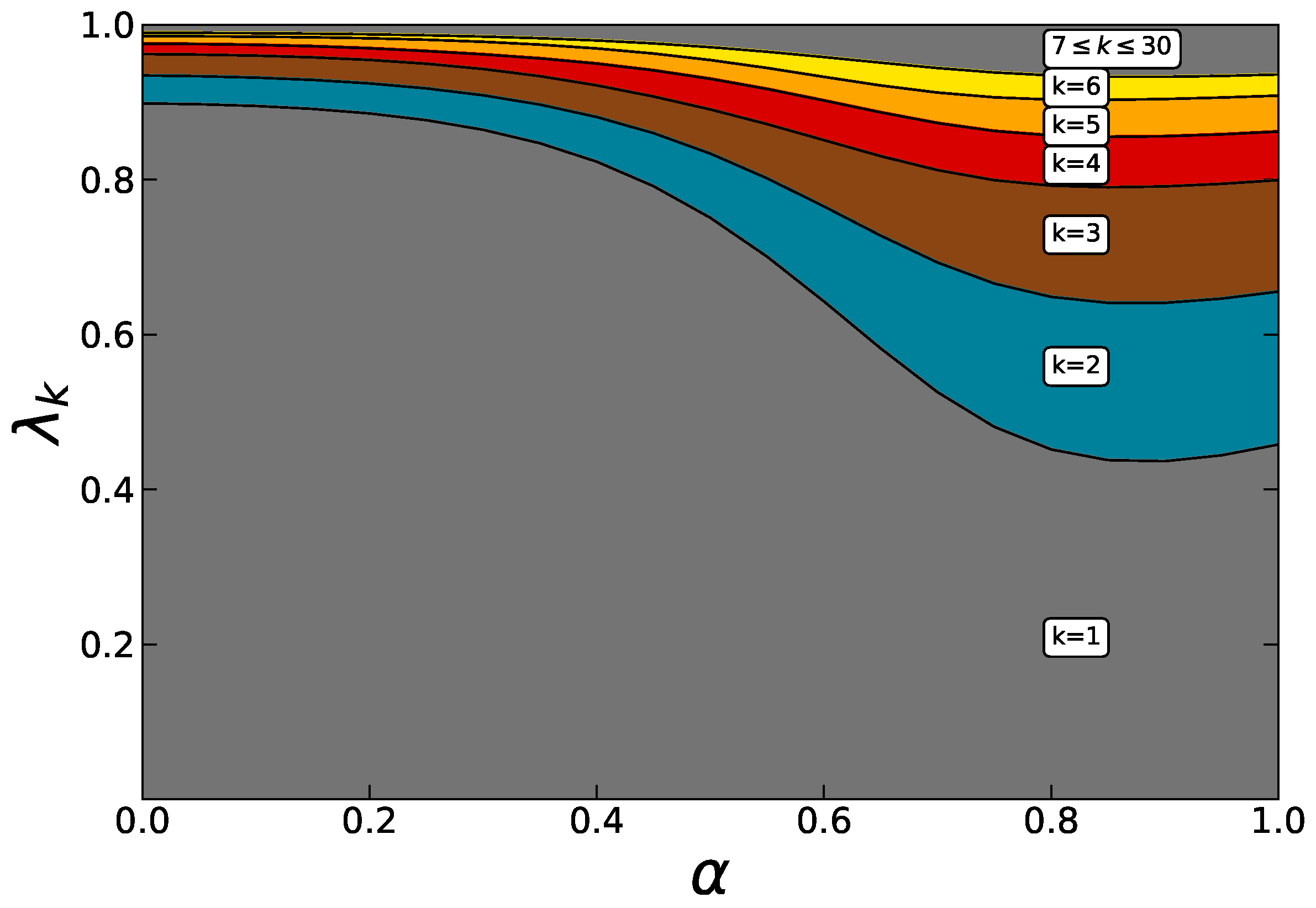
Figure 4.
The three principal mismatch components for .

Figure 5.
(a) Intraday and (b) seasonal amplitude profiles of the three principal components for . The intraday profiles have been obtained by averaging the amplitudes over all days of the underlying eight years while keeping the intraday hour fixed. For the seasonal profiles the amplitudes have been first averaged over a day, and then over the eight years while keeping the day of the year fixed.

Figure 6.
The six principal mismatch components for .
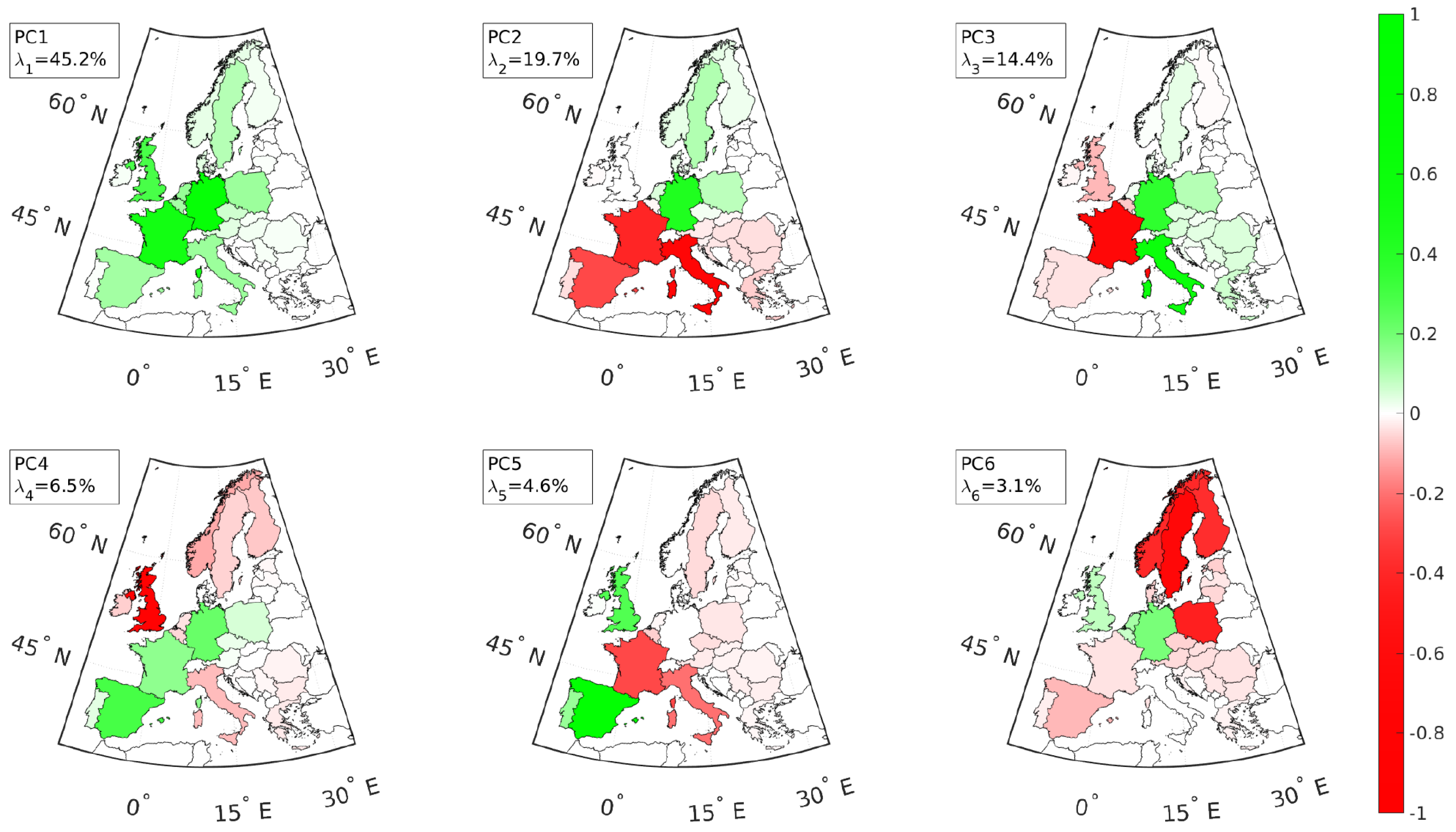
Figure 7.
(a) Intraday and (b) seasonal amplitude profiles of the first three principal components for . The seasonal amplitude profiles for and have been artificially shifted by −0.5 and −1.0, respectively.
Figure 7.
(a) Intraday and (b) seasonal amplitude profiles of the first three principal components for . The seasonal amplitude profiles for and have been artificially shifted by −0.5 and −1.0, respectively.

Figure 8.
Decomposed eigenvalues (from the bottom) and (from the top) as a function of the renewable mix . The solar share increases towards , and the wind share increases towards . The white band in the middle represents .
Figure 8.
Decomposed eigenvalues (from the bottom) and (from the top) as a function of the renewable mix . The solar share increases towards , and the wind share increases towards . The white band in the middle represents .

Table 1.
Various infrastructure measures as a function of the truncation parameter K used for the PCA approximation (18).
Table 1.
Various infrastructure measures as a function of the truncation parameter K used for the PCA approximation (18).
| , | |||||||
|---|---|---|---|---|---|---|---|
| 0.0301 | 0.0281 | 0.0272 | 0.0258 | 0.0238 | 0.0195 | 0.0136 | |
| 0.0101 | 0.0101 | 0.0098 | 0.0098 | 0.0096 | 0.0095 | 0.0089 | |
| 0.1402 | 0.1388 | 0.1371 | 0.1368 | 0.1365 | 0.1348 | 0.1318 | |
| 0.686 | 0.682 | 0.659 | 0.656 | 0.650 | 0.643 | 0.613 | |
| 0.0184 | 0.0164 | 0.0154 | 0.0139 | 0.0119 | 0.0077 | 0.0020 | |
| 0.0120 | 0.0101 | 0.0091 | 0.0074 | 0.0061 | 0.0040 | 0.0007 | |
| 1.812 | 1.486 | 1.372 | 1.250 | 1.156 | 0.904 | 0.356 |
© 2017 by the authors. Licensee MDPI, Basel, Switzerland. This article is an open access article distributed under the terms and conditions of the Creative Commons Attribution (CC BY) license (http://creativecommons.org/licenses/by/4.0/).
Share and Cite
MDPI and ACS Style
Raunbak, M.; Zeyer, T.; Zhu, K.; Greiner, M. Principal Mismatch Patterns Across a Simplified Highly Renewable European Electricity Network. Energies 2017, 10, 1934. https://doi.org/10.3390/en10121934
AMA Style
Raunbak M, Zeyer T, Zhu K, Greiner M. Principal Mismatch Patterns Across a Simplified Highly Renewable European Electricity Network. Energies. 2017; 10(12):1934. https://doi.org/10.3390/en10121934
Chicago/Turabian StyleRaunbak, Mads, Timo Zeyer, Kun Zhu, and Martin Greiner. 2017. "Principal Mismatch Patterns Across a Simplified Highly Renewable European Electricity Network" Energies 10, no. 12: 1934. https://doi.org/10.3390/en10121934
Note that from the first issue of 2016, this journal uses article numbers instead of page numbers. See further details here.