1. Introduction
A significant portion of the global energy consumption is due to the consumption of buildings and thus the corresponding share of the building sector in the total energy consumption in India, Europe and USA is around 40% [
1,
2]. Previous studies have demonstrated that around half of the energy demand of buildings can be attributed to their heating, ventilation and air-conditioning (HVAC) systems [
3]. Accordingly, the consumption of air-conditioning systems has a significant impact on the electrical grid and the precise prediction of its variations can provide the grid management with notable benefits such as competitiveness in the day-ahead market, dispatch management, demand-side management and control optimization. Apparently, a straightforward solution in order to simulate the behaviour of buildings, and thus predicting the variations in their HVAC consumption, is developing physical models employing their geometrical and construction characteristics [
4], infiltration properties, required ventilation rate, occupancy profiles and other details. However, grid management firms and utilities do not commonly have access to such details about the characteristics of their consumers’ buildings.
One potential solution to deal with the mentioned issue is the development of data-driven models, which correlate the consumed power of air conditioners in the individual buildings with the corresponding ambient and temporal conditions and can thus estimate harsh variations in HVAC consumption due to changes in the ambient conditions. Nevertheless, the latter approach requires installing dedicated meters permanently connected to the HVAC equipment in each individual building and consequently results in additional costs for the user or the utility firm.
Another alternative approach, which is implemented in the present study, is to utilize the aggregate consumed power of individual buildings, which is obtained from smart meters. Once the aggregate consumed power at each time step is obtained, energy disaggregation methodologies are employed in order to determine the corresponding share of air-conditioning consumption. In order to train the disaggregation algorithm, a very short (one week) measurement period with additional meters for individual devices, is needed. However, the latter requirement can eventually be evaded once a database with abundant measured data corresponding to the operation of different combinations of various residential devices is available. The ubiquitous spread of smart meters throughout the world, and specifically in industrialized countries, facilitates utilizing the proposed approach.
The disaggregation of aggregate data by non-intrusive method was first proposed by Hart, Kern and Schweppe at Massachusetts Institute of Technology (MIT) in the 80s and was further developed by Hart and termed Non-Intrusive Appliance Load Monitoring (NALM), in the 90s [
5]. Supervised NALM algorithms utilize a set of the labelled signatures, e.g., voltage and current waveforms, of electrical devices in order to identify them from the aggregate load. This requires a one-time intrusion intervention in the household of interest where each device is identified and labelled based on its unique signature. In unsupervised NALM, the algorithm undergoes training and the devices are clustered from the aggregate waveform by matching either ON/OFF signals, voltage or current spikes in the aggregate data. The clustering is a way of labelling the devices and performing NALM with total non-intrusiveness. For the actual disaggregation, appliance models such as ON/OFF, Finite State Machine (FSM) and Continuously Variable proposed by Hart [
6] along with Zero-Loop-Sum-Constraint, are utilized owing to their corresponding simplicity and ease of developing disaggregation algorithms. Combinatorial Optimisation and Factorial Hidden Markov models, which are elaborated in
Section 3, are two widely employed state-of-the-art energy disaggregation algorithms, which are accordingly employed in the present work.
The second step of the present work is focused on utilizing machine-learning algorithms to conduct short-term prediction of air-conditioning load employing the data obtained from the disaggregation step. Many previous studies had investigated the possibility of using machine-learning algorithms for predicting the energy demand of buildings. Anstett and Kreider [
7] employed artificial neural networks to predict the daily energy consumption in a complex institutional building. Jain et al. [
8] developed a similar approach using Support Vector Machine (SVM), based on an empirical dataset from a multi-family residential building, aimed at predicting the overall energy consumption. They also examined the effect of temporal granularity on the resulting prediction and their results demonstrated an overall coefficient of variation (CV) of 11.4, 0.54 and 0.08 on a daily, hourly and 10 min data granularity respectively. In the latter study, the CV metric was defined as the square root of squares of deviations of the predicted and the actual values divided by the number of samples multiplied by the mean. Chen et al. [
9] performed a short-term prediction of electric demand in the building sector via hybrid SVM and compared it with pure SVM. A relative improvement in mean absolute error of 6% was achieved. Artificial neural networks were utilized by Karatasou et al. [
10] to predict hour-ahead and day-ahead energy consumption in buildings employing two different datasets from the Energy Predictions Shootout I contest and an office building in Athens. The prediction results showed a CV of 2.39–5.59 and 2.57–24.35 for hour-ahead and day-ahead prediction applied on the first and the second datasets respectively. Edwards et al. [
11] conducted a study focused on prediction of residential loads employing various algorithms including regression, Feed Forward Neural Network (FFNN), Support Vector Machine (SVM), Least-Square Support Vector Machine (LS-SVM), Hierarchical Mixture of Experts (HME) and Fuzzy C-Means (FCM) on the ASHRAE Great Energy Prediction Shootout with 15 min granularity and utilizing the Campbell Creek house database. Their results demonstrated that an average CV values of 36.38, 31.83, 29.55, 27.62, 35.78, 28.35, 27.94 obtained by Regression, FFNN, Support Vector Regression (SVR), LS-SVM, HME-Regression, HME-FFNN and FCM-FFNN respectively. Basu et al. [
12] developed a general model using a knowledge driven and data driven approach. The model was tested over IRISE of REMODECE datasets using different machine learning algorithms including Neural Networks, Nearest Neighbours and Decision Tree. Elevated prediction accuracies were obtained and were reported to be around 94.7%, 94.1% and 94.5% for lighting, washing machine and oven consumptions. Dong et al. [
13] developed a hybrid model through data-driven techniques employing ANN, SVM, (LS-SVM), Gaussian process regression (GPR) and Gaussian mixture model (GMM) on four different residential data for hour ahead and day ahead forecast of AC load. The hybrid models performed slightly better than those in the works of Jain et al. [
8] and Edwards et al. [
11]. Dong et al. [
14] discussed a similar approach using SVM and focused on optimizing the model’s hyper parameters for predicting building energy consumption in tropical regions. However, in this work each model was built to yield maximum accuracy whilst predicting hour-ahead and day-ahead AC energy consumption. Kontokosta et al. [
15] developed a predictive model using Linear Regression, SVM and Random Forest approaches to predict city-scale energy use in buildings in New York. It was shown that SVM performed the best among them. Owing to the availability of the building area and geo-location, the energy consumptions were correlated with the building area, occupants and floors. Li et al. [
16] performed particle swarm optimization based LS-SVM for building cooling prediction. They found that the hyper-parameters of the model could be quickly optimized while attempting to conduct predictions for nonlinear and time series dataset like energy consumption. Fan et al. [
17] developed a method for short-term cooling load prediction using supervised and unsupervised learning algorithm with deep neural network. Li et al. [
18] used back propagation neural network, radial basis function neural network, general regression neural network and SVM for predicting the hourly cooling load in office buildings. Yao et al. [
19] developed a combined forecast model based on analytic hierarchy process for day-ahead prediction. Analytic hierarchy process is a simple decision making procedure based on setting priorities. González et al. [
20] modelled a feedback artificial neural network for hourly energy consumption in buildings. The model was not optimized based on the number of neurons, however they seemed to perform well on predicting the energy consumption. Ben-Nakhi et al. [
21] developed a general regression neural network (GRNN) to predict cooling loads in buildings in Kuwait using a dataset from 1997–2001. The prediction model also used temperature forecast to aid in day-ahead predictions. Apart from machine-learning, genetic algorithms are also a promising method of analysing building energy performance. Castelli et al. [
22] developed a model using genetic programming approach with geometric semantic genetic programming (GSGP). The model predicted both heating and cooling load of a set of residential buildings.
As previously pointed out, the present study involves two main steps. The first step is focused on extracting the air-conditioning consumption from the aggregate smart meter data of a building. The second step is dedicated to building a machine-learning model to predict hour-ahead and day-ahead consumption of air conditioner units from the obtained data. Yearly consumption data of a residential building, provided by Pecan Street Inc.’s Dataport™ [
23] was utilized. Combinatorial Optimisation (CO) and Factorial Hidden Markov Model (FHMM) algorithms, which are implemented in the open source Non-Intrusive Load Monitoring Toolkit (NILMTK) [
24], have been utilized to conduct the disaggregation step. The obtained air-conditioning load and the corresponding historical weather and time-related features are then employed as input features of the prediction procedure. The time-related data includes the hour, the day of the week, the weekday/weekend, and day/night, while the temperature and the irradiance constitute the employed weather data. The ambient temperature is provided within the dataset and, in order to include the effect of irradiance, the time-stamped generation of a nearby photovoltaic plant, is utilized. The use of Photovoltaics (PV) generation as an indication of irradiance will increase the general applicability of the proposed method, as the grid managers have access to PV production at various locations, while the irradiance measurement devices are not ubiquitous.
Hour-ahead and day-ahead predictions are finally performed using several machine-learning algorithms such as Linear Regression, Random Forest Decision Tree, Support Vector Machines, and Multi-Layer Perceptron Neural Networks and their corresponding results are compared.
It is worth mentioning that the principal objective of the present work is performing short-term prediction of AC loads while only employing the aggregate data obtained from a conventional smart meter and in the absence of other detailed information about the building including the construction characteristics, occupancy, the ventilation rate, technical details of the air-conditioning unit, and other details. The latter situation is a problem that the utility companies and grid management units are commonly facing as they attempt to predict the aggregate power consumption of users (out of which a notable share is related to AC consumption) only employing the total consumed power communicated by the smart meter. However, they do not have access to any other information regarding the details of the building construction or the behaviour of the occupants. Hence, the main novelty of the present work, compared to previously conducted data-driven residential load prediction studies, is attempting to obtain increased accuracy while not having access to the mentioned detailed information about the building and its occupants.
2. Employed Dataset
The dataset used in the present work is the yearly consumption data of a residential building, located in Austin (TX, USA), which is measured in the year 2014, and is publicly accessible via Dataport™ (provided by Pecan Street Inc., Austin, TX, USA). This dataset includes the total consumed power of the house along with the power consumed by individual devices recorded with 1-min sampling rate. The devices include a split air conditioner, dish washer, washing machine, electric oven, water pumps, electric heater, fridge, fans, electric water heater, micro wave oven, toaster, television, miscellaneous electronic devices (laptops, tablets) and light bulbs of different types (fluorescent, incandescent, and light-emitting diodes (LED).
The database also contains ambient temperature with 1-hour sampling rate which was added as a feature to the machine-learning model. As previously mentioned, in order to take into account, the effect of irradiance, time-stamped power generation of a photovoltaic unit installed on a nearby building has also been employed. Although detailed information regarding the model and the orientation of the PV panels, utilized in the unit, is not accessible, the corresponding power generation at any specific hour is proportional to the irradiance in that hour.
3. Energy Disaggregation Methodology
Energy disaggregation estimates appliance-by-appliance electricity consumption from a single meter that measures the total household’s electrical consumption. First step in disaggregation is to establish appliance models, which describe the behaviour and electrical signature of appliance. There are several device models but the most simple and common models are the ON/OFF, Finite State Machines (FSM) and Continuously Variable [
25]. The ON/OFF model considers that an appliance may be either ON or OFF at any given point in time. While it is ON there is no other state that the appliance may take (e.g., toaster, lights vacuum cleaners). FSM model considers appliances, which have several distinct switching states during ON mode. The appliance passes through different states every time the devices is used (e.g., washing machines, electric rice cooker, clothes dryer). The Continuously Variable model includes appliances like light dimmers, and variable-speed hand tools. These devices are very difficult to identify and disaggregate from the whole home energy data. It relies on high frequency harmonics to identify such devices. Appliance signatures like voltage, real and reactive power, current, root mean square (RMS) current, steady state harmonics and phase shifts are the electrical marks on the aggregate data from which appliances can be identified. The methods under the steady state make use of appliance signatures when the load is in steady state operation [
26]. Appliances, whenever switched ON, have a transient state momentarily before reaching a steady state which is caused by the sudden change in the circuit [
27]. Transient behavior of most electrical appliances is unique, which makes it convenient for identification and disaggregation. The drawback, however, is the need for high sampling rate which may increase the cost of measurement and computation. Hybrid signatures are combination of steady-state signatures and transient signatures. H. H. Chang et al. [
28,
29] combined steady-state real power, reactive power and total transient energy to disaggregate different appliances with the same real and reactive power. Apart from steady-state and transient signatures, there are other methods of using features as signatures which need not be extracted from the measured appliance data. Hour of the day, frequency of appliance usage, usage duration and distribution over the day and the correlation between the usage of other appliances are some features which can be used to increase accuracy of identification and disaggregation [
30]. Energy disaggregation, ultimately is to provide estimates [
24],
, of the actual power demand,
yt(n), of each appliance
n at time
t, from the household’s aggregate power readings,
yt. Generally, NALM algorithms are developed over the appliance models mentioned above. The NILMTK toolkit [
24] uses
xt(n) ∈ Z > 0 to represent the ground truth state, and
to represent the appliance state estimated by the disaggregation algorithm.
The basic process of disaggregation can be divided into seven steps. Firstly, the whole house aggregate electricity data is collected through sensors or smart meters at the utility interface which measures the average power and the RMS voltage on the mains with a standard sampling interval (kHz, 1 s, 1 min, 15 min). Step 2 is to normalize the total load power or the measured signature with respect to the fluctuation in the mains. Supply voltage to consumers may have plodding or discrete changes due to factors like load-dependent voltage drops in transmission lines and transformers. This may lead to detecting step changes that may interfere with our appliance signature and ultimately with the disaggregation. The toolkit implements Hart’s method based on linear model where admittance is preferred over power and current as a signature. The admittance
Y(t) is given by Equation (1), where
P(t) and
V(t) are the measured power and RMS voltage. The normalized power is then expressed as in Equation (2), which is admittance corrected by a constant value, resulting in a power normalized to 120 V. Step 3 involves passing the normalized power of the aggregate data through the edge detector, which evaluates time and size of all the step changes. It involves signal processing techniques like filtering, differentiating to detect peaks and to capture the step changes caused by appliance state changes. For an unsupervised learning algorithm, where the appliance labels are unavailable, more electrical signatures, such as reactive power, are considered when evaluating the step changes of unique devices. The detected step changes (e.g., ON/OFF) when mapped on the real-complex
∆P-∆Q space, could be grouped into clusters based on equal and opposite components. Finally, each step changes are matched with the corresponding cluster in case of unsupervised learning or to appliances in case of supervised learning [
24].
3.1. Combinatorial Optimization
The total load depends on which appliance are switched on at any given moment, so a switching process, vector
a(t) is defined. The vector
a(t) is an
n component Boolean vector defining the state of
n appliances at time
t:
For
i = 1,…,
n, the switch process modulates the power consumption of the individual appliances. A multiphase load with
p phases can be modelled as a
p-vector in which each component is the load on one phase. Then we model the measured power given by Equation (4). Where
P(t) is the
p-vector as seen at the utility at time
t, and
e(t) is a small noise or error term. Equation (4) suggests a straightforward criterion for estimating the state of the individual appliances. If all
n of the
P; are known and the measured power
P(t) is given, at each
t choose the
n vector
a(t) which minimizes |
e(t)|, under the constraint that
a is an
n-dimensional Boolean vector [
5]:
This is a familiar combinatorial optimization problem. Each time instant is a separate optimization problem and each time instant is independent. Combinatorial optimization is a subset sum problem and even with scalar
P variables it’s an
NP complete “weighted set” problem. The computation becomes taxing as it is exponential with the number of appliances [
5].
3.2. Factorial Hidden Markov Model
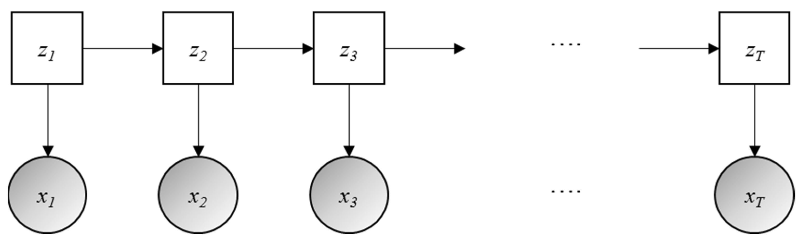
Hidden Markov Models (HMM) are temporal graphical models which are probabilistic methods. A simple representation of HMM is show in
Figure 1 [
31]. Several machine learning and artificial intelligence models implement Markov models. A well-known example is in the area of speech recognition [
32] and word prediction. The HMM is sequence of discrete variables in which each variable emits a single continuous variable, which is dependent upon the value of the discrete variable. The discrete variables (sequence
z =
z1,…,
zT) are not observed whereas the continuous variables (sequence
x =
x1,…,
xT) are observed.
T is the length of the sequence or the time step of each discrete variable. Each discrete variable
zT can correspond to one of
K states, while each continuous variable can take on any real number. The three mains parameters describing a HMM are initial probability, transition probability and emission probability.
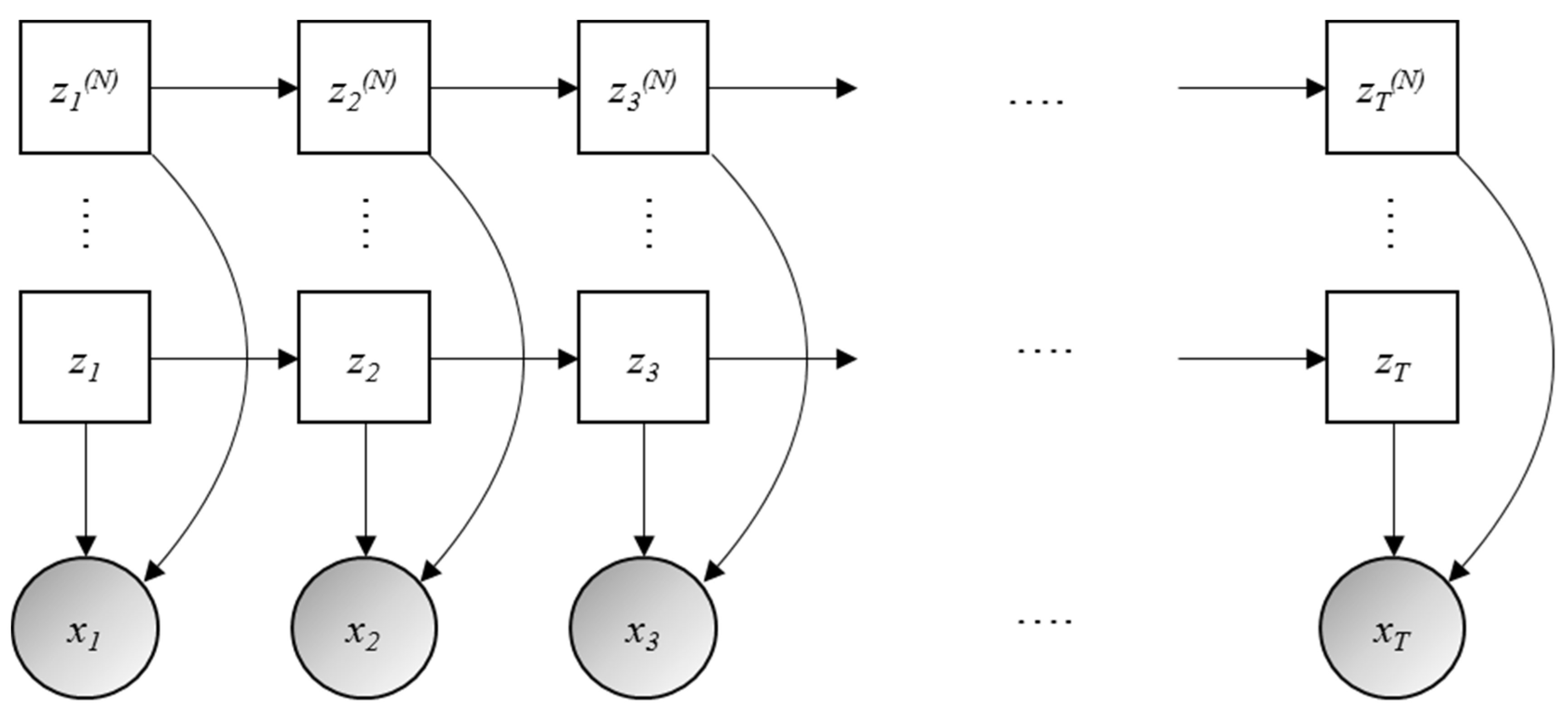
Factorial Hidden Markov Models (FHMM) are a type of HMM wherein there are several independent Markov chains of hidden variables,
z(1),…,
z(N), in which
N is the number of chains. Therefore, each continuous observed variable is dependent on multiple hidden variables [
33]. The
Figure 2 is a representation of a Factorial Hidden Markov model. Similar to a HMM, the joint likelihood of a FHMM is given by Equation (6), where 1:
N represents a sequence of appliances 1…,
N. The complexity of both learning and inference is greater for FHMMs than HMMs. The computational cost is exponential in the number of chains,
N, the model will therefore become computationally intractable for large
N [
31]:
In the FHMM, each of the n devices in a building is considered as a Hidden Markov Model. Each device has a discrete hidden state, denoted xt(i) ∈ for any given time t for device i, which corresponds approximately to the internal state of the device (ON/OFF or one of intermediate states if it were an FSM). At each time t, given the internal state, the ith device produces a Gaussian distributed power, represented xt(i), with state-specific mean and variance parameters.
Since, we only observe the sum of all the power outputs at each time as in Equation (7) [
31]:
With a smart meter, in a practical scenario, the disaggregation task can then be framed as an inference problem. Given an observed sequence of aggregate energy
x1,…,
xT, we aim to compute the posterior probability of the individual device consumptions x
t(i) for
i = 1,…,
n and
t = 1, . . . ,
T [
34].
6. Discussion
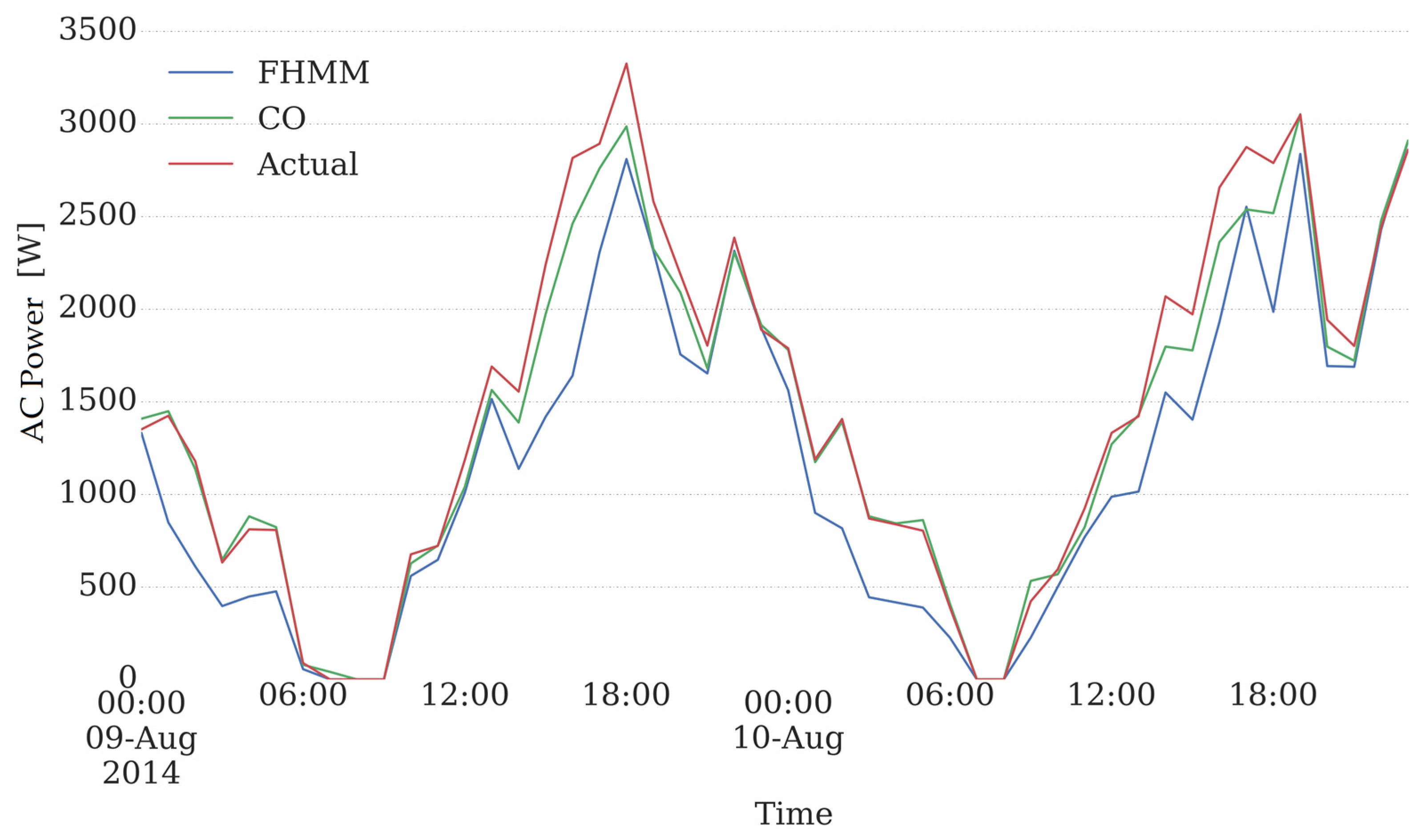
The results of the disaggregation step demonstrated that only employing a short training period (one week) and using combinatorial optimization, which is a simple disaggregation algorithm with a low computational cost, an elevated yearly disaggregation accuracy (98.67%) can be achieved. Furthermore, a complete database including electrical signatures obtained from different combinations of domestic appliances can be employed as a training dataset; thus, the training period, with dedicated sensors for different devices, can accordingly be avoided. Therefore, it can be concluded the disaggregation step is not a practical impediment to the proposed method and does neither introduce a notable error in the prediction procedure, as the disaggregation accuracies are notably high.
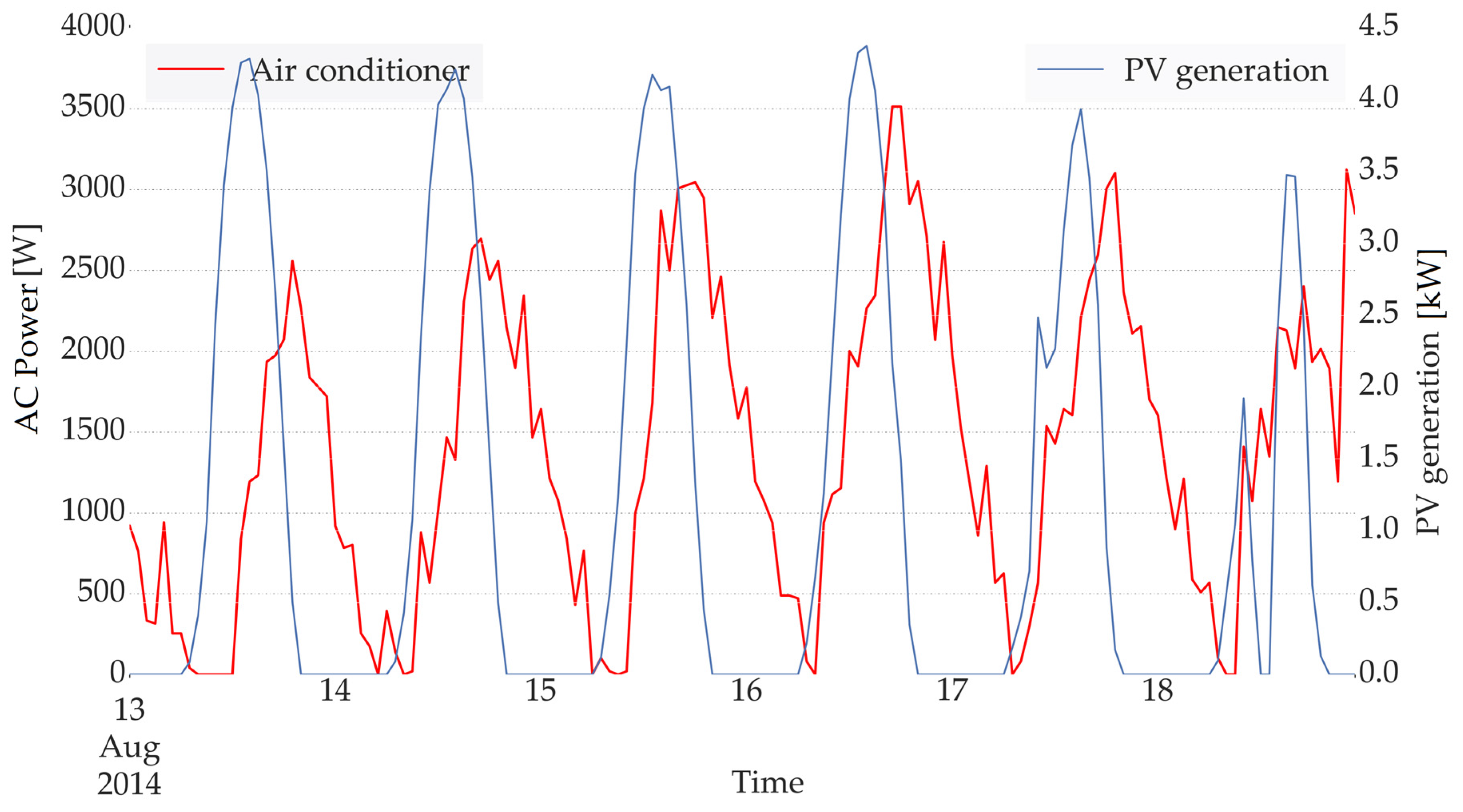
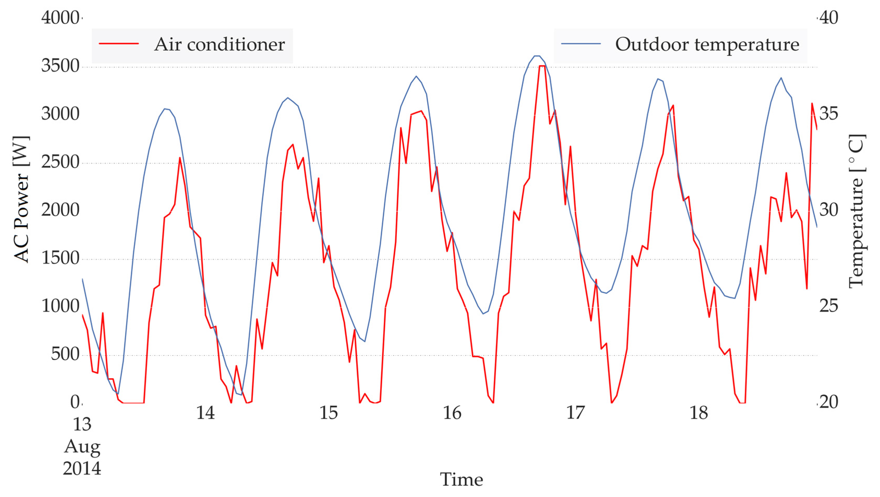
The investigation on the correlation between the AC consumption and the ambient condition, demonstrated the expected lag between an increment in the ambient temperature and the resulting rise in the AC consumption. The observed lag is due to the thermal storage of the walls, which results in a delay in the conversion of temperature increment to an increase in the AC load. Furthermore, an even larger time lag was observed while investigating the effect of solar irradiation (through generation profile of a nearby PV plant). The latter lag is due to the delay in the conversion of the radiation heat transfer into a convective one, as the incident solar irradiation will first heat up the walls and the objects inside the building (through windows) and they will in turn warm up the internal air through convection. Accordingly, the predicted ambient temperature of the next hour along with the corresponding values in the last 5 h were chosen as the inputs while the PV generations with the lag of 5 and 6 h were taken into account to represent solar irradiation. The latter demonstrates the importance of having the knowledge and keeping in mind the physical behaviour of buildings even while employing a purely data-driven approach.
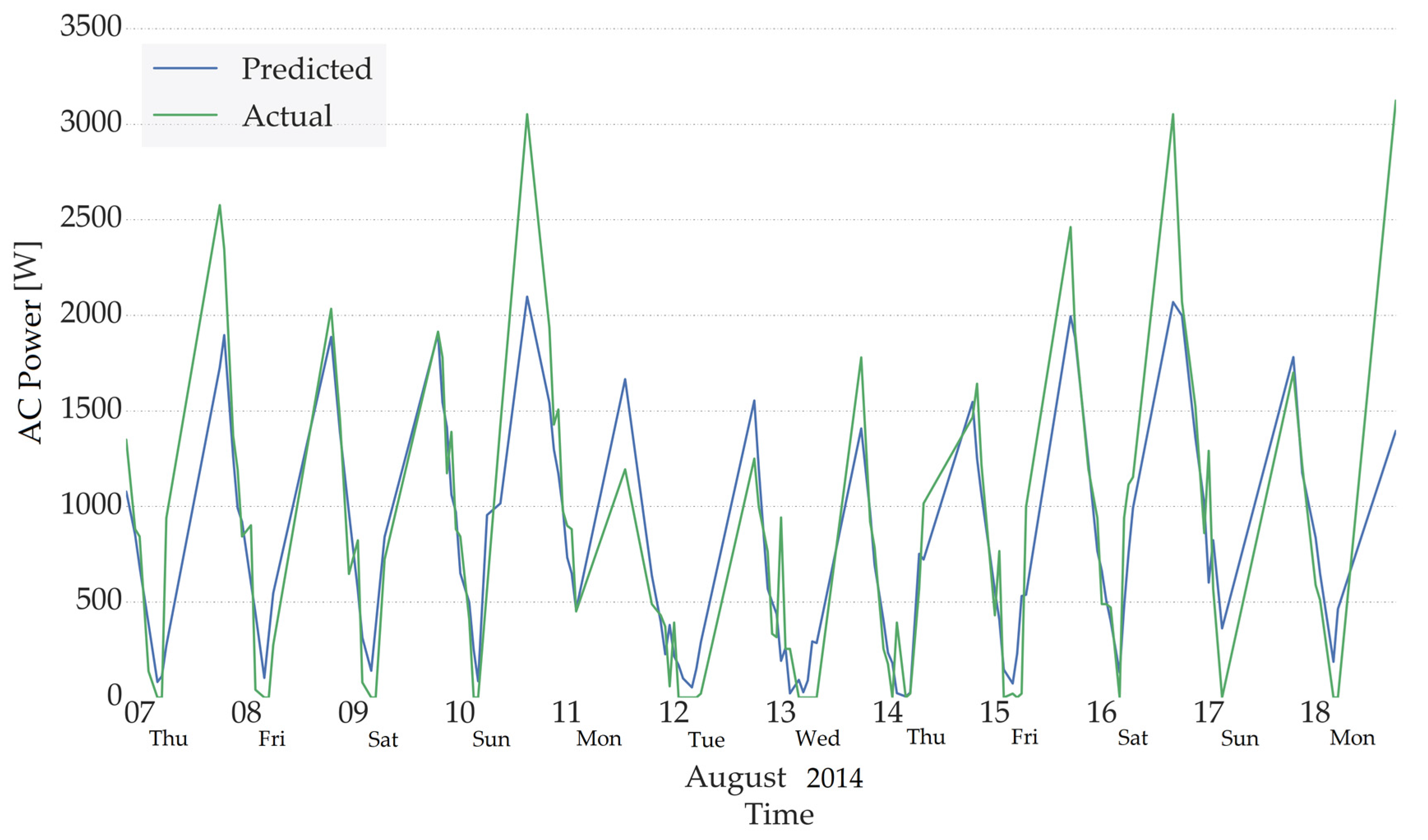
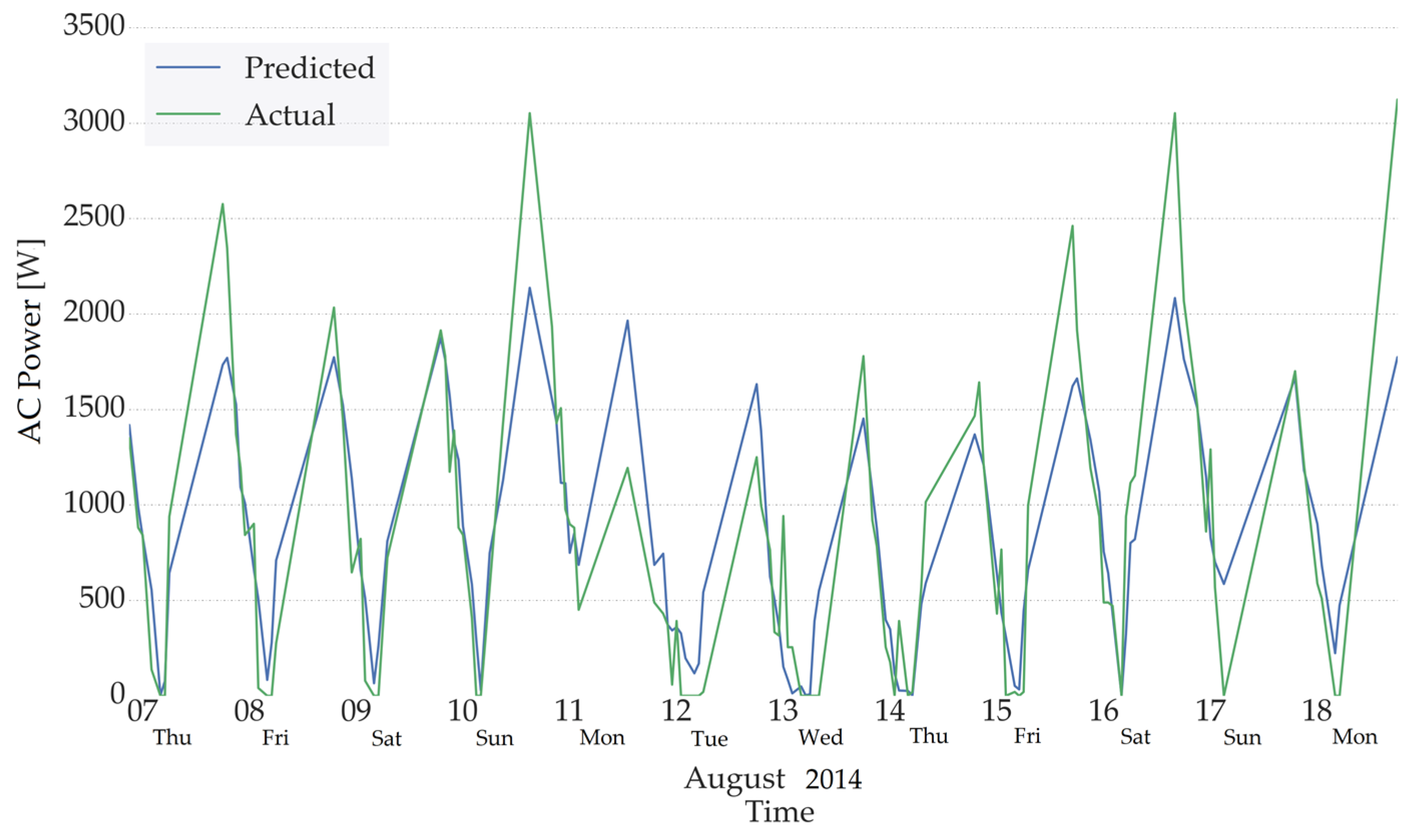
The results of hour-ahead and day-ahead prediction demonstrates the fact that using the proposed approach elevated accuracies can be obtained while only the aggregate load data and historical weather data is available and no information regarding the building characteristics or occupants’ behaviour was given. The latter is owing to the fact that providing the AC consumption for several time steps and the corresponding ambient temperature and PV generation (representing solar irradiation), while applying the appropriate time lags, facilitates simulating the physical behaviour of the building in an implicit way. Furthermore, considering the seasonality related parameters (hour, day of the week, weekday/weekend), and the consumption profiles in the previous hours, provides information regarding the occupancy profile in an indirect manner. The fact that outside weather condition are included can even result in a better prediction of occupancy as the occupants will be more willing to stay at home and use the air-conditioner at the hours with high ambient temperature and elevated solar irradiation. The level of the latter willingness is apparently learnt from similar conditions taking place in the previous measured periods.
However, the latter information is not enough in order to predict the non-repeating alterations (peaks) in the behaviour of the occupants. These alterations commonly happen in the weekends and the prediction results demonstrated that the developed models could not anticipate such sudden and non-repeating variations.


