A Simplified Top-Oil Temperature Model for Transformers Based on the Pathway of Energy Transfer Concept and the Thermal-Electrical Analogy

Abstract

This paper presents an alternative approach to determine the simplified top-oil temperature (TOT) based on the pathway of energy transfer and thermal-electrical analogy concepts. The main contribution of this study is the redefinition of the nonlinear thermal resistance based on these concepts. An alternative approximation of convection coefficient, h, based on heat transfer theory was proposed which eliminated the requirement of viscosity. In addition, the lumped capacitance method was applied to the thermal-electrical analogy to derive the TOT thermal equivalent equation in differential form. The TOT thermal model was evaluated based on the measured TOT of seven transformers with either oil natural air natural (ONAN) or oil natural air forced (ONAF) cooling modes obtained from temperature rise tests. In addition, the performance of the TOT thermal model was tested on step-loading of a transformer with an ONAF cooling mode obtained from previous studies. A comparison between the TOT thermal model and the existing TOT Thermal-Electrical, Exponential (IEC 60076-7), and Clause 7 (IEEE C57.91-1995) models was also carried out. It was found that the measured TOT of seven transformers are well represented by the TOT thermal model where the highest maximum and root mean square (RMS) errors are 6.66 °C and 2.76 °C, respectively. Based on the maximum and RMS errors, the TOT thermal model performs better than Exponential and Clause 7 models and it is comparable with the Thermal-Electrical 1 (TE1) and Thermal-Electrical 2 (TE2) models. The same pattern is found for the TOT thermal model under step-loading where the maximum and RMS errors are 5.77 °C and 2.02 °C.

1. Introduction

Thermal modeling is one of the important studies for the estimation of the top-oil temperature (TOT) and hot-spot temperature (HST) in transformers. TOT is defined as the average of the tank outlet oil temperature and the oil pocket temperature [1]. Meanwhile, HST consists of ambient temperature (AT), TOT rise, and HST rise [1]. One of the common approaches to carry out thermal modeling of transformers is through a numerical network thermal model. Currently, there are two standards that utilize this approach to determine HST and TOT, known as IEC 60076-7 and IEEE C57.91-1995 [1,2]. These standards use the exponential function for constant loading and the differential function for dynamic loading for determination of HST and TOT [1,2]. A number of studies were also carried out to develop alternative thermal models for HST and TOT [3,4,5,6,7,8,9,10,11,12,13,14,15,16,17,18]. The majority of these studies were carried out based on the thermal-electrical analogy that represents the heat transfer equivalent circuit in the form of a resistor capacitor (RC) circuit [3]. Based on this concept, the current source analogy represented the heat input due to losses, whilst the nonlinear resistance analogy represented the effect of air or oil cooling convection currents [3].

TOT is one of the important components to determine HST in transformers. A model based on the thermal-electrical analogy was developed [5,6] to determine the TOT thermal model. In these studies, the nonlinear thermal resistance was expanded through inclusion of the Nusselt, Prandtle, and Grashof numbers. The loss variation, viscosity changes with temperature, equivalent thermal capacitances, oil time constants for different designs, and oil circulation were also considered in [5,6,7]. The TOT obtained by TOT thermal model in [5] was quite close to the measured TOT, as compared to Annex G model in IEEE C57.91-1995 for transformers with oil natural air forced (ONAF) and oil forced air forced (OFAF) cooling modes. The same finding was found for transformers with either oil natural air natural (ONAN) or ONAF, and OFAF cooling modes in [6]. The TOT thermal models in [5,6,7] utilize a number of input parameters which increase the accuracy of the simulated TOT. A Levenberg–Marquardt model was proposed in [8] to determine the input parameters, such as TOT rise at rated, oil time constant, and constant n, based on in-service TOT measured data. Based on the case study of transformers with ONAF and OFAF cooling modes, it was found that the TOT thermal model based on the Levenberg–Marquardt approach could represent the measured TOT better than the Clause 7 model in IEEE C57.91-1995 [8]. This model requires the in-service measured TOT information, which may not be available for some transformers in order to determine the input parameters. A TOT thermal model was introduced in [9,10] based on the concept of outdoor and indoor heat transfer flows of transformers. The indoor TOT thermal model equivalent circuit required a considerable number of thermal resistances input parameters, such as windings, oil, core, tank, cooling air, ventilation holes, walls, and ceiling. The model also considered the heat generated in the distribution cabinet, $q_{cabin}$, such as heat from busbars, fuses, disconnectors, and switches. Based on the case study of a transformer with an ONAN cooling mode, the TOT thermal model could represent quite well the measured TOT for indoor and outdoor conditions. The TOT thermal models in [9,10] are beneficial for comprehensive thermal analysis for individual outdoor or indoor transformers.

Nonlinear thermal resistance is one of the important parameters in the thermal-electrical analogy thermal models. This parameter was commonly determined based on the Nusselt, Prandtle, and Grashof numbers according to heat transfer theory [5,8,9,10,11]. Through this approach, the oil viscosity was included in the final form of the nonlinear thermal resistance equation due to its sensitivity toward temperature. The viscosity coefficient was also calibrated in [12] in order to determine the nonlinear thermal resistance for the transformer with a rating over 6300 kVA. Another approach to determine the nonlinear thermal resistance was based on measured values outside the tank and average winding temperatures from the short-circuit heating experiment in [19]. The nonlinear thermal resistance was represented by an exponential form in [20,21] where the element of the heat conductance matrix and constants were determined based on a genetic algorithm (GA) [20,21]. Recently, a moisture-dependent nonlinear thermal resistance was proposed in [22] where it considered the cellulose thermal conductivity and area/thickness.

This paper presents a simplified approach to estimate the TOT based on a proposed concept of the pathway of energy flow that is adopted from heat transfer theory to construct the nonlinear thermal resistance and lumped capacitance circuit. An alternative approximation of the convection coefficient, h, is proposed, which eliminates the requirement of the viscosity for application in the thermal-electrical analogy. The main contribution of this study is the application of the pathway of energy based on heat transfer principles and the redefinition of nonlinear thermal resistance. The derivation of the TOT thermal model is presented and tested based on the measured TOT of seven transformers with either ONAN or ONAF cooling modes. The TOT thermal model is also tested with the step-loading of a transformer with an ONAF cooling mode from previous studies.

2. Heat Transfer Theory Application in Transformers

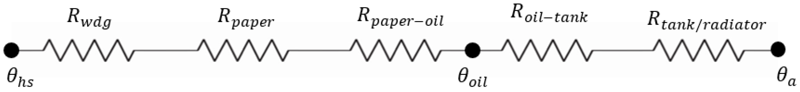
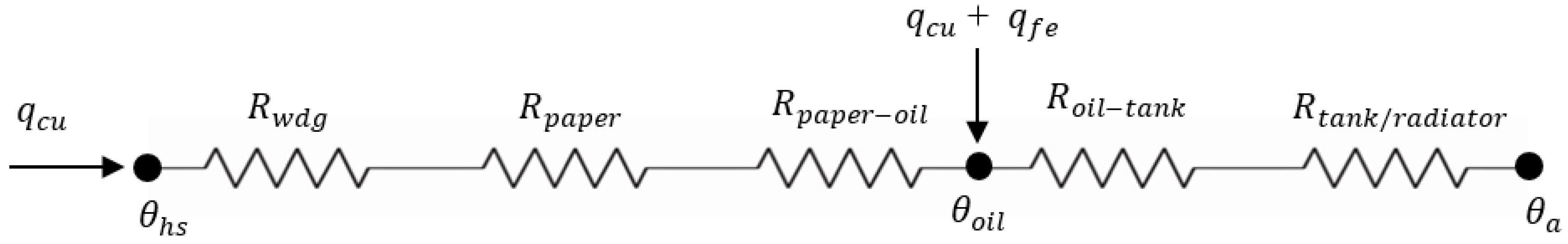
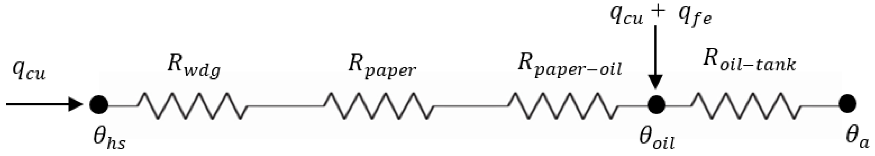
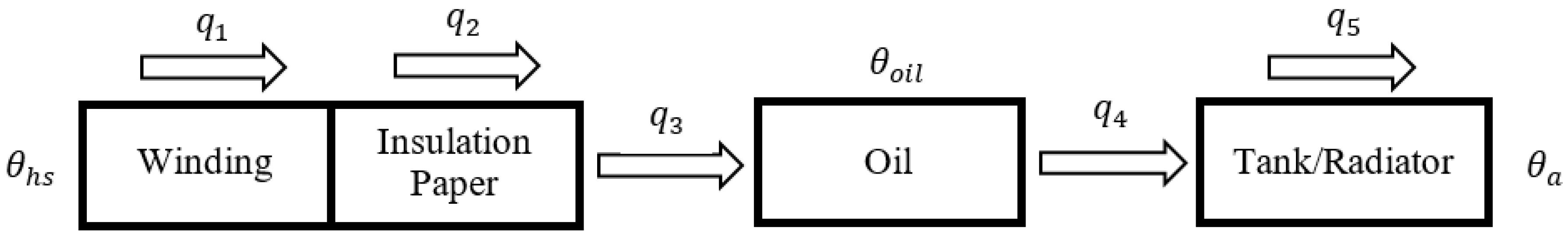
2.1. Concept of Heat Transfer in Transformers

The concept of energy transfer is one of the simplest approaches to evaluate the heat transfer in transformers. In general, heat transfer occurs when there is a temperature difference in a medium or between media [23]. In transformers, the heat sources originate from load and no-load losses which distribute through oils and transfer to the tank/radiator of the transformer [24]. HST is the hottest temperature inside a transformer and is normally located at windings, and the coolest temperature is AT, which is located outside the transformer. Based on the heat transfer theory, heat or energy will transfer from the hottest temperature to the coolest temperature; in transformers, from HST to the AT via conduction and convection through all media, including windings, insulation papers, oils, and tanks/radiators. This pathway of energy transfer concept is applied in this study to determine the thermal resistance equivalent circuit, which can be seen in Figure 1.

Where $q_1$ is the conduction through copper of the winding, $q_2$ is the conduction through the insulation paper, $q_3$ is the convection from insulation paper to the oil, $q_4$ is the convection from the oil to the tank, $q_5$ is the conduction through the tank/radiator of transformers, ${\theta }_{hs}$ is the HST, ${\theta }_{oil}$ is the TOT, and ${\theta }_a$ is the AT. Comprehensive analysis of the thermal conductivity through insulation paper can be characterized based on consideration on the porous characteristics. Fractal geometry is among the common approaches that can be used to model the pore structure for modelling the thermal conductivity through insulation paper [25,26]. In this study, the thermal conductivity of insulation paper was represented by a single thermal resistance for the simplification of the thermal resistance equivalent circuit.

2.2. Nonlinear Thermal Resistances

All media in transformers have their own thermal resistances which act like dissipation elements. The thermal resistance is nonlinear due to the presence of the convection coefficient, h. Detailed descriptions of the nonlinear thermal resistance are presented in Section 3.1. Based on the pathway of energy transfer concept shown in Figure 1, the heat transfer thermal resistance equivalent circuit is represented by Figure 2.

According to Figure 2, there are three locations of temperatures, which are ${\theta }_{hs}$, ${\theta }_{oil}$, and ${\theta }_a$. The heat sources in transformers originate from load losses, $q_{cu}$, and no-load losses, $q_{fe}$, which are added in the thermal resistance equivalent circuit, as shown in Figure 3.

Previous study showed that the thermal resistance of tank/radiator could be discarded due to the perfect conductor characteristic where the thermal resistance was practically close to zero [3]. In this study, the focus is on the TOT thermal resistance that relates with the convection thermal resistance of the oil to the tank. Due to this reason, the application of Fourier’s law of heat conduction and the dual phase lag method are not considered in the computation. The final form of the heat transfer thermal resistance equivalent circuit can be re-drawn, as shown in Figure 4.

2.3. Lumped Capacitance

The current form of the thermal resistance equivalent circuit in Figure 4 can only be used under steady state condition. In order to determine HST and TOT under transient, the lumped capacitance approach was applied. The Biot number of the thermal resistance must be determined before this approach can be implemented. The Biot number is the ratio of the thermal resistance of conduction over the convection [3,23]. In transformers, the Biot number is less than 1 since the thermal resistance of conduction is normally smaller than convection [3]. Through application of the lumped capacitance method, the capacitance is added to the heat transfer thermal resistance equivalent circuit which can be represented by Figure 5. There are two capacitances that are included, known as oil and winding capacitances. Each of the capacitances represent the storage element of either the oil or winding in the thermal resistance equivalent circuit.

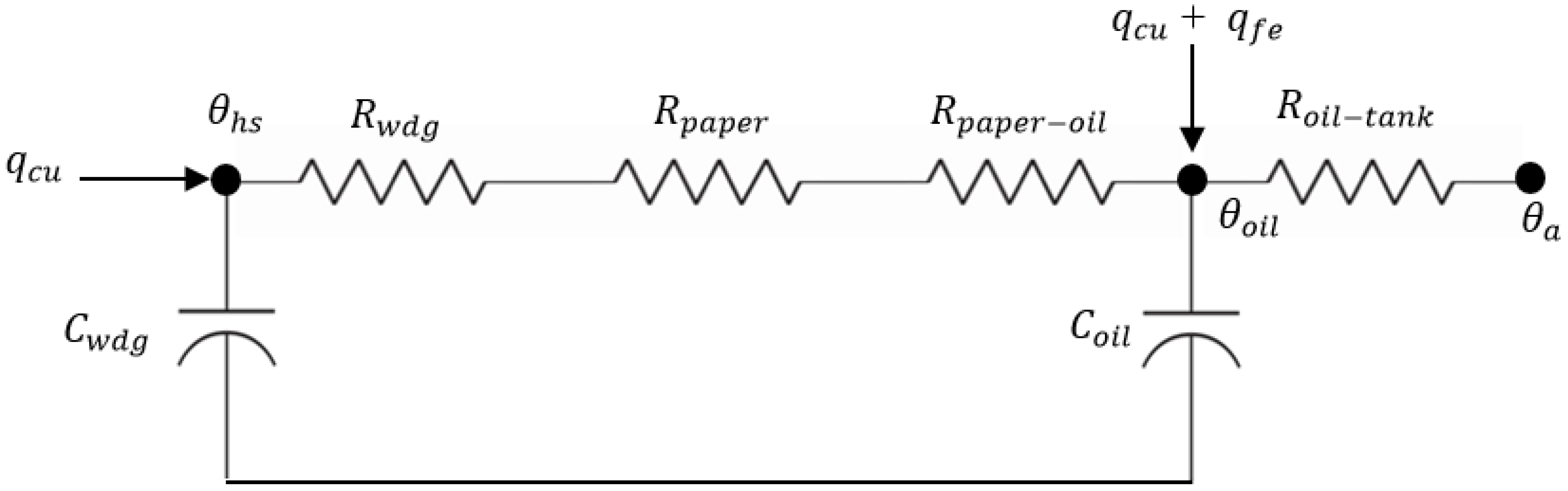
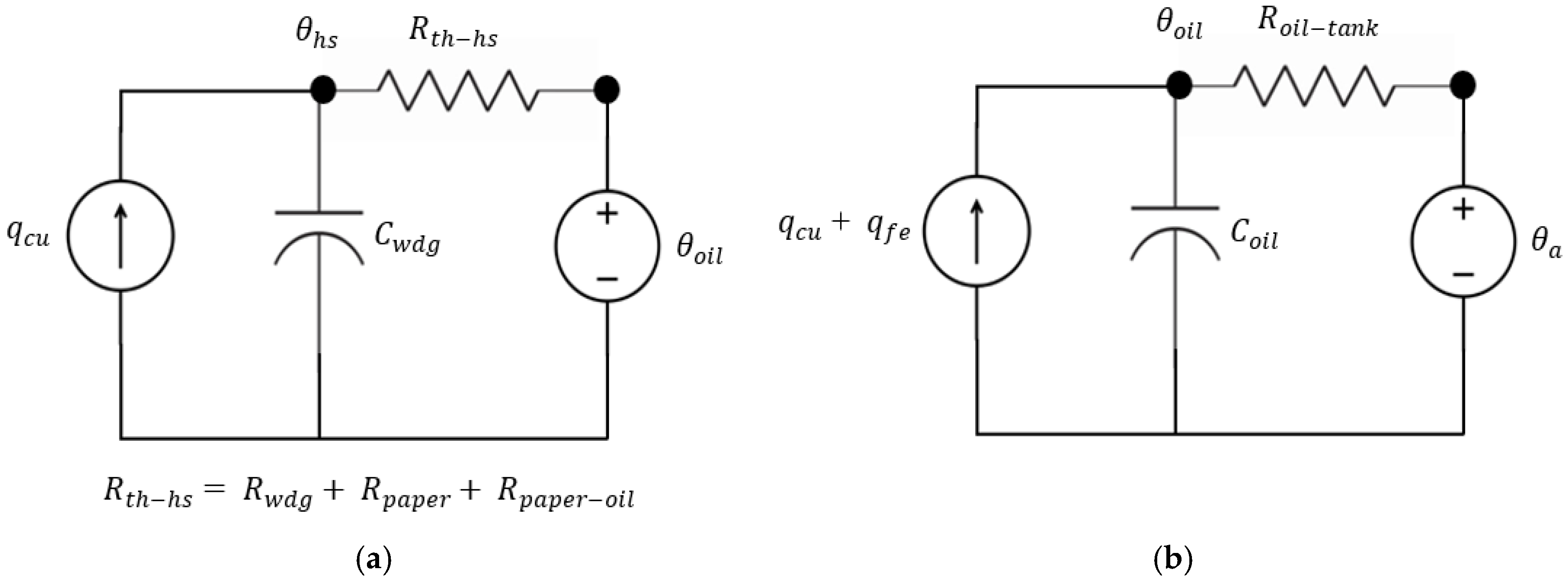
2.4. Thermal-Electrical Analogy

The thermal-electrical analogy parameters are through variable, across variable, dissipation element, and storage element [3]. The through variable, heat source, q, in the thermal approach is analogous to current, I in the electrical approach. Meanwhile, the across variable, temperature, $\theta$, in the thermal approach is analogous to voltage, v, in the electrical approach. The dissipation element variable, thermal resistance, $R_{th}$, in the thermal approach is analogous to electrical resistance, $R_{el}$, in the electrical approach, while the storage element variable, thermal capacitance, $C_{th}$, in the thermal approach is analogous to electrical capacitance, $C_{el}$, in the electrical approach. Based on Figure 5 the thermal-electrical circuit can be divided into two models, known as the HST and TOT models, as shown in Figure 6a,b, respectively. In this study, only the TOT model was developed and examined.

3. Top-Oil Temperature Thermal Model

3.1. Definition of Nonlinear Oil Thermal Resistance

According to the heat transfer theory in [5,23], the nonlinear oil thermal resistance is defined as the inverse product of convection coefficient, h and area, A which is given by Equation (1). The nonlinear oil thermal resistance, $R_{oil}$ in Equation (1) refers to nonlinear oil-to-tank thermal resistance, $R_{oil-tank}$ in Figure 6b:

$$R_{oil}=\frac{1}{hA}$$

(1)

The convection coefficient, h in Equation (1) may be affected by multiple factors, including the medium thermal characteristics. According to the heat transfer theory, the convection coefficient, h varies with the temperature difference between the object (transformers tank/radiator) and the fluid (transformers oil) [23]. In this case, h is approximated by the expression in Equation (2) [23]:

$$h=C{\left({\theta }_s-{\theta }_{\infty }\right)}^n$$

(2)

where n and C are constants and the unit of C is W/m²·K⁽¹⁺ⁿ⁾. The constant, n, contributes to the nonlinearity of the convection coefficient, h. In Equation (2), ${\theta }_s$ represents the TOT, ${\theta }_{oil}$, and ${\theta }_{\infty }$ represents the AT, ${\theta }_a$. The TOT rise, $∆{\theta }_{oil}$, is determined by subtracting ${\theta }_a$ from the ${\theta }_{oil}$ where it can be simplified to Equation (3):

$$h=C{\left(∆{\theta }_{oil}\right)}^n$$

(3)

Substitution of Equation (3) into Equation (1) leads to the final proposed equation of nonlinear oil thermal resistance as shown in Equation (4):

$$R_{oil}=\frac{1}{CA{\left(∆{\theta }_{oil}\right)}^n}$$

(4)

The thermal resistance is nonlinear due to the presence of the constant n, which represents the heat transfer convection modes in transformers, as shown in Equation (4).

The redefinition of the nonlinear oil thermal resistance based on approximation of convection coefficient, h, in Equation (4) is among the key contributions of this study. A comparison with similar forms of nonlinear thermal resistances such as Susa and Tang models was also carried out. The nonlinear thermal resistance for Susa Model can be obtained based on the following approach. The relationship of Nusselt, Prandtle, and Grashof numbers is given by Equation (5) [5]:

$$N_u=C{\left[G_r·P_r\right]}^n$$

(5)

The Nusselt, Prandtle, and Grashof numbers can be determined based on Equations (6)–(8):

$$N_u=\frac{h·L}{k}$$

(6)

$$P_r=\frac{c_{oil}·\mu }{k}$$

(7)

$$G_r=\frac{L^3·{\rho }_{oil}{}^2·g·\beta ·(∆{\theta }_{oil})}{{\mu }^2}$$

(8)

Substitutions of Equations (6)–(8) into Equation (5) lead to the Equation (9):

$$\frac{h·L}{k}=C·{\left[\frac{L^3·{\rho }_{oil}{}^2·g·\beta ·(∆{\theta }_{oil})}{{\mu }^2}·\frac{c_{oil}·\mu }{k}\right]}^n$$

(9)

Since only viscosity is sensitive toward temperature, Equation (9) can be reduced to Equation (10) known as the convection coefficient, h [5]:

$$h=C_1·{(\frac{∆{\theta }_{oil}}{\mu })}^n$$

(10)

where $C_1$ is obtained from Equation (11):

$$C_1=C·{\left[{\rho }_{oil}{}^2·g·\beta ·k^{\left(\frac{1-n}{n}\right)}·L^{\left(\frac{3n-1}{n}\right)}·c_{oil}\right]}^n$$

(11)

Substitution of Equation (10) into (1) leads to Equation (12) which is the final form of the nonlinear thermal resistance for Susa model [5]:

$$R_{oil}=\frac{{\mu }^n}{CA{\left(∆{\theta }_{oil}\right)}^n}$$

(12)

The nonlinear thermal resistance for Tang model can be derived based on the following approach. According to [20,21], the thermal conductance can be represented by Equation (13):

$$G=a{\left(∆{\theta }_{oil}\right)}^b$$

(13)

where G is the element of the thermal conductance matrix, $∆{\theta }_{oil}$ is the TOT rise, a and b are the constants. The reciprocal of Equation (13) leads to the final form of nonlinear thermal resistance for Tang model, as shown in Equation (14) [20,21]:

$$R_{oil}=\frac{1}{a{\left(∆{\theta }_{oil}\right)}^b}$$

(14)

The proposed nonlinear thermal resistance does not consider viscosity as in the Susa model. The nonlinear thermal resistance in the Susa model considers multiple oil parameters, such as characteristic length, L, oil thermal conductivity, k, specific heat of oil, $c_{oil}$, oil density, ${\rho }_{oil}$, gravitational constant, $g$, and oil thermal expansion coefficient, β, while the proposed nonlinear thermal resistance only considers the constant C that is derived from the heat transfer theory. The derivation of nonlinear thermal resistance in the Susa model is different from the proposed nonlinear thermal resistance where it is based on Nusselt, Prandtle, and Grashof numbers. Meanwhile, the nonlinear thermal resistance in the Tang model is derived based on the exponential form of heat conductance matrix element. The constants, a and b in the Tang model are obtained based on GA through the in-service measured data.

3.2. Derivation of Top-Oil Temperature Thermal Model

Based on the TOT thermal-electrical analogy equivalent circuit in Figure 6b, the differential equation representation can be determined based on Equation (15) [5]:

$$q_{fe}+q_{cu}=C_{oil}\frac{d{\theta }_{oil}}{dt}+\frac{\left({\theta }_{oil}-{\theta }_a\right)}{R_{oil}}$$

(15)

Substitution of Equation (4) into Equation (15) leads to Equation (16):

$$q_{fe}+q_{cu}=C_{oil}\frac{d{\theta }_{oil}}{dt}+\frac{\left({\theta }_{oil}-{\theta }_a\right)}{\frac{1}{CA{\left(∆{\theta }_{oil}\right)}^n}}$$

(16)

The nonlinear oil thermal resistance at rated, $R_{oil,rated}$, TOT rise at rated, $∆{\theta }_{oil,rated}$, and oil time constant, ${\tau }_{oil}$, can be determined according to Equations (17)–(19):

$$R_{oil,rated}=\frac{1}{CA{\left(∆{\theta }_{oil,rated}\right)}^n}$$

(17)

$$∆{\theta }_{oil,rated}={\left(q_{fe}+q_{cu}\right)}_{rated}·R_{oil,rated}$$

(18)

$${\tau }_{oil}=R_{oil,rated}·C_{oil}$$

(19)

The ratio of load losses at the rated to the no load losses, R can be computed according to Equation (20):

$$R=\frac{q_{cu}}{q_{fe}}$$

(20)

The ratio of the load current to the load current at rated, K can be calculated according to Equation (21):

$$K=\frac{I}{I_{rated}}$$

(21)

Substitutions of Equations (17)–(21) into Equation (16) lead to Equation (22), which is the final form of the TOT thermal model:

$$\frac{1+R·K^2}{1+R}·∆{\theta }_{oil,rated}={\tau }_{oil}\frac{d{\theta }_{oil}}{dt}+\frac{{\left({\theta }_{oil}-{\theta }_a\right)}^{1+n}}{∆{\theta }_{oil,rated}{}^n}$$

(22)

The TOT thermal model in Equation (22) is in the same form as in [8], however the approach in terms of derivation of the TOT thermal model is different. The nonlinear oil thermal resistance, $R_{oil}$, in [8] was obtained through Nusselt, Prandtle, and Grashof numbers. The TOT model in [8] also took into consideration on the influence of oil viscosity in the TOT thermal model. In addition, the input parameters such as the TOT rise at rated, $∆{\theta }_{oil,rated}$, oil time constant, ${\tau }_{oil}$ and constant, n, in [8] were estimated based on the Levenberg-Marquardt method. The TOT thermal model in Equation (22) does not require the information on the viscosity for determination of nonlinear oil thermal resistance, $R_{oil}$ where simplification is carried out through approximation of convection coefficient, h, of the heat transfer convection between the oil and the transformer tank.

3.3. Input Data

The TOT thermal model was tested on seven transformers with ONAN and ONAF cooling modes. The seven transformers were named as TX1, TX2, TX3, TX4, TX5, TX6, and TX7. In addition, the TOT thermal model was also tested on the step loading of a 250 MVA transformer with ONAF cooling mode obtained from [1,5] and named as TX8. Both TX3 and TX4 have identical design except the cooling mode for TX3 is ONAN and TX4 is ONAF. The input parameter for these transformers ratings are shown in

Table 1. Input parameters for the TOT thermal model.

Parameters	Transformer/Winding
	TX1	TX2	TX3	TX4	TX5	TX6	TX7
	11/0.433 kV	33/11 kV	33/11 kV	33/11 kV	132/11 kV	132/33 kV	132/33 kV
Rating (kVA)	300	15,000	30,000	30,000	30,000	60,000	90,000
Cooling Modes	ONAN	ONAF	ONAN	ONAF	ONAN	ONAN	ONAF
Load (p.u.)	1.00	1.00	1.00	1.00	1.00	1.00	1.00
R	4.52	7.56	10.47	11	5.79	4.66	10
$∆{\theta }_{oil,rated}$ (K)	30.3	51.23	59.2	58.87	38.9	44.07	47.87
${\tau }_{oil}$ (min)	129	152	200	207	239	295	165
${\theta }_{oil,i}$ (K)	31.9	44.9	29.7	29.9	31.8	32.3	41.7
(IEC) Oil exponent, x	0.8	0.8	0.8	0.8	0.8	0.8	0.8
(IEC) Constant, $k_{11}$	0.5	0.5	0.5	0.5	0.5	0.5	0.5
(IEEE) Exponent, n	0.8	0.9	0.8	0.9	0.8	0.8	0.9

for constant loading and

Table 2. Input parameter for TOT thermal model for step loading [1,5].

Parameters	Transformer/Winding
	TX8
	250/118 kV
Rating (kVA)	250,000
Cooling Modes	ONAF
Load (p.u.)	1.00 pu/3 h + 0.60 pu/3 h + 1.50 pu/2 h + 0.30 pu/3 h + 2.10 pu/0.33 h
R	10.17
$∆{\theta }_{oil,rated}$ (K)	38.3
${\tau }_{oil}$ (min)	168
${\theta }_{oil,i}$ (K)	38.3

for step loading. The oil time constant, ${\tau }_{oil}$, was calculated based on [2] using the input parameters obtained from the nameplate rating such as the weight of core and coil in kg, the weight of the tank and fittings in kg, and transformer oil in L. Based on the convection heat transfer, the value of constant, n is 0.25 for laminar oil circulation [27], which indicates free convection (ONAN cooling modes). It is used to control the sensitivity of the TOT model curve which depends on the cooling modes and oil circulation of transformers. The constant, n, has different values for forced convection (ONAF and OFAF cooling modes) [5,6]. In this study, the constant n for TE1 and TE2 were calibrated based on the measured TOT in order to increase the accuracy of the simulated TOT. The same procedure was carried out for the TOT thermal model, which can be seen in

Table 3. Constant n used in this study.

Transformers	Constant n
	TE1	TE2	Thermal Model
TX1	0.1	1	0.1
TX2	0.75	0.9	1
TX3	0.75	0.9	1
TX4	0.75	0.9	1
TX5	0.4	0.95	0.65
TX6	0.4	0.95	0.65
TX7	0.25	0.95	0.5
TX8	0.1	0.95	0.25

.

3.4. Comparison with Previous Thermal-Electrical and Standard Models

In this study, two thermal-electrical models in [3,5] were used to evaluate the performance of the TOT thermal model. Thermal-Electrical 1 (TE1) model was proposed by [5] as seen in Equation (23). The model in Equation (24) was introduced by [3] and termed as Thermal-Electrical 2 (TE2) model:

$$\frac{1+R·K^2}{1+R}·{\mu }_{pu}{}^n·∆{\theta }_{oil,rated}={\mu }_{pu}{}^n·{\tau }_{oil}\frac{d{\theta }_{oil}}{dt}+\frac{{\left({\theta }_{oil}-{\theta }_a\right)}^{1+n}}{∆{\theta }_{oil,rated}{}^n}$$

(23)

$$\frac{1+R·K^2}{1+R}·{\left(∆{\theta }_{oil,rated}\right)}^{\frac{1}{n}}={\tau }_{oil}\frac{d{\theta }_{oil}}{dt}+{\left({\theta }_{oil}-{\theta }_a\right)}^{\frac{1}{n}}$$

(24)

The TOT thermal model was also compared with the existing models in standards known as the Exponential model in IEC 60076-7 and the Clause 7 model in IEEE C57.91-1995, as seen in Equations (25) and (26) [1,2]. The constants, x, $k_{11}$, and n used for both the Exponential and Clause 7 thermal models were chosen based on Table 1.

$${\theta }_{oil}={\theta }_a+∆{\theta }_{oil,i}+\left(∆{\theta }_{oil,rated}·{\left[\frac{1+R·K^2}{1+R}\right]}^x-∆{\theta }_{oil,i}\right)·f_1$$

(25)

$${\theta }_{oil}={\theta }_a+\left(∆{\theta }_{TO,U}-∆{\theta }_{TO,i}\right)·\left[1-e^{\frac{-t}{{\tau }_{oil}}}\right]+∆{\theta }_{TO,i}$$

(26)

Maximum error and root mean square (RMS) error were used to analyze the simulated TOT, as can be seen in Equations (27) and (28):

$$maximumerror=\left|{\theta }_{oil,calculated}-{\theta }_{oil,measured}\right|$$

(27)

$$RMSerror=\sqrt{\frac{{{\displaystyle \sum }}_{i=1}^n{\left({\theta }_{oil,calculated}-{\theta }_{oil,measured}\right)}^2}{n}}$$

(28)

where ${\theta }_{oil,measured}$ is the measured TOT, ${\theta }_{oil,simulated}$ is the simulated TOT, and n is the number of samples.

4. Results and Discussions

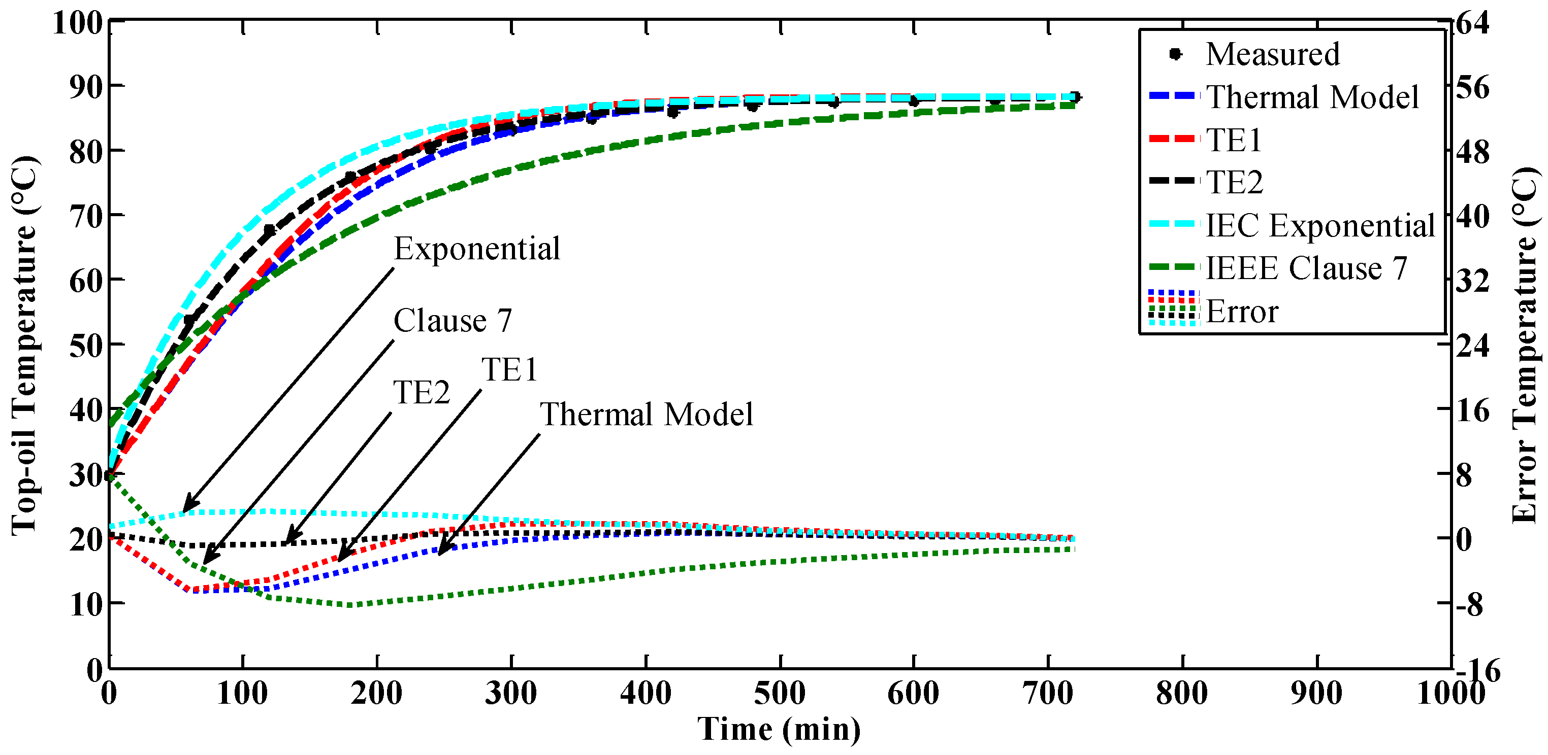
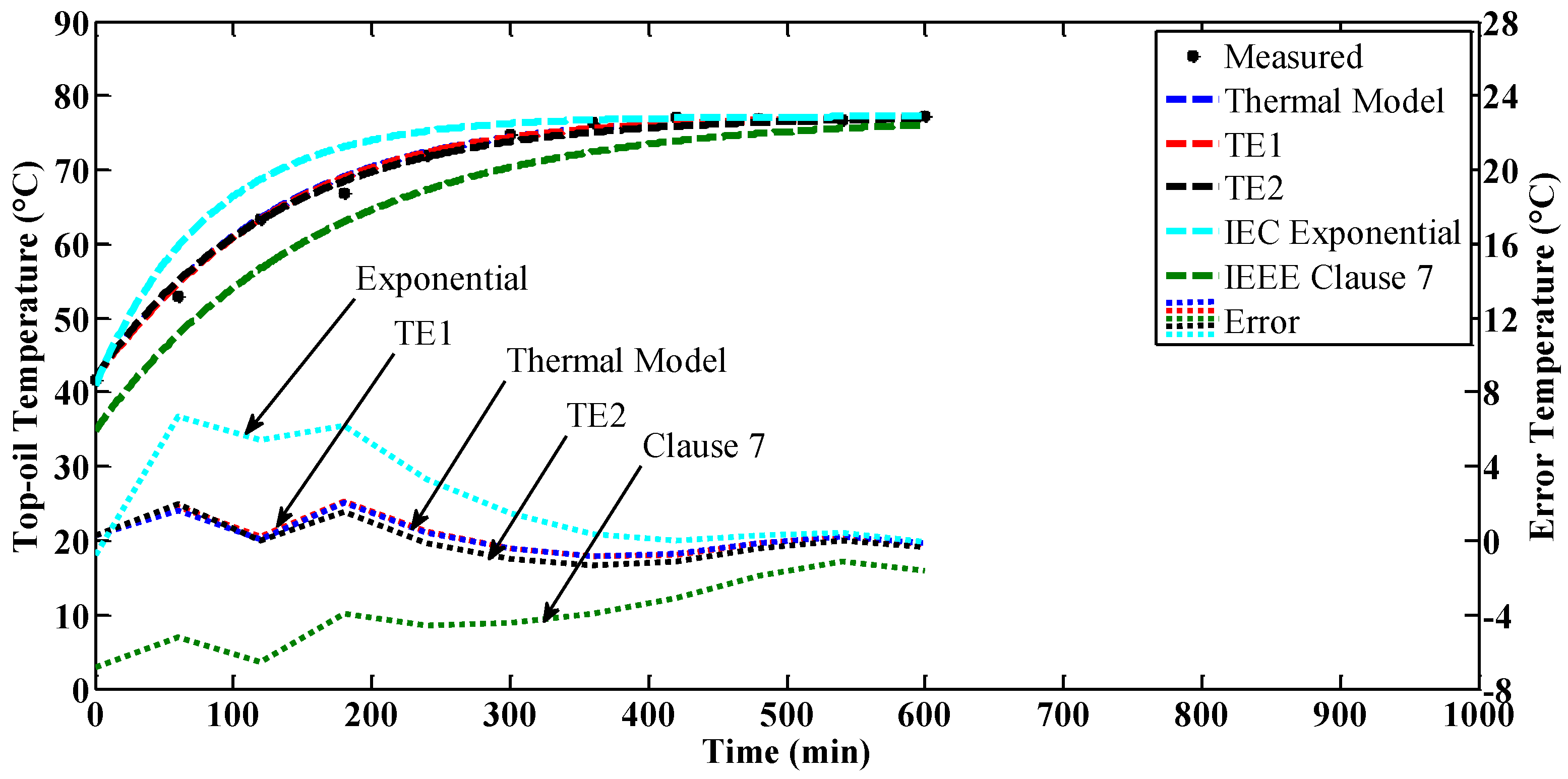
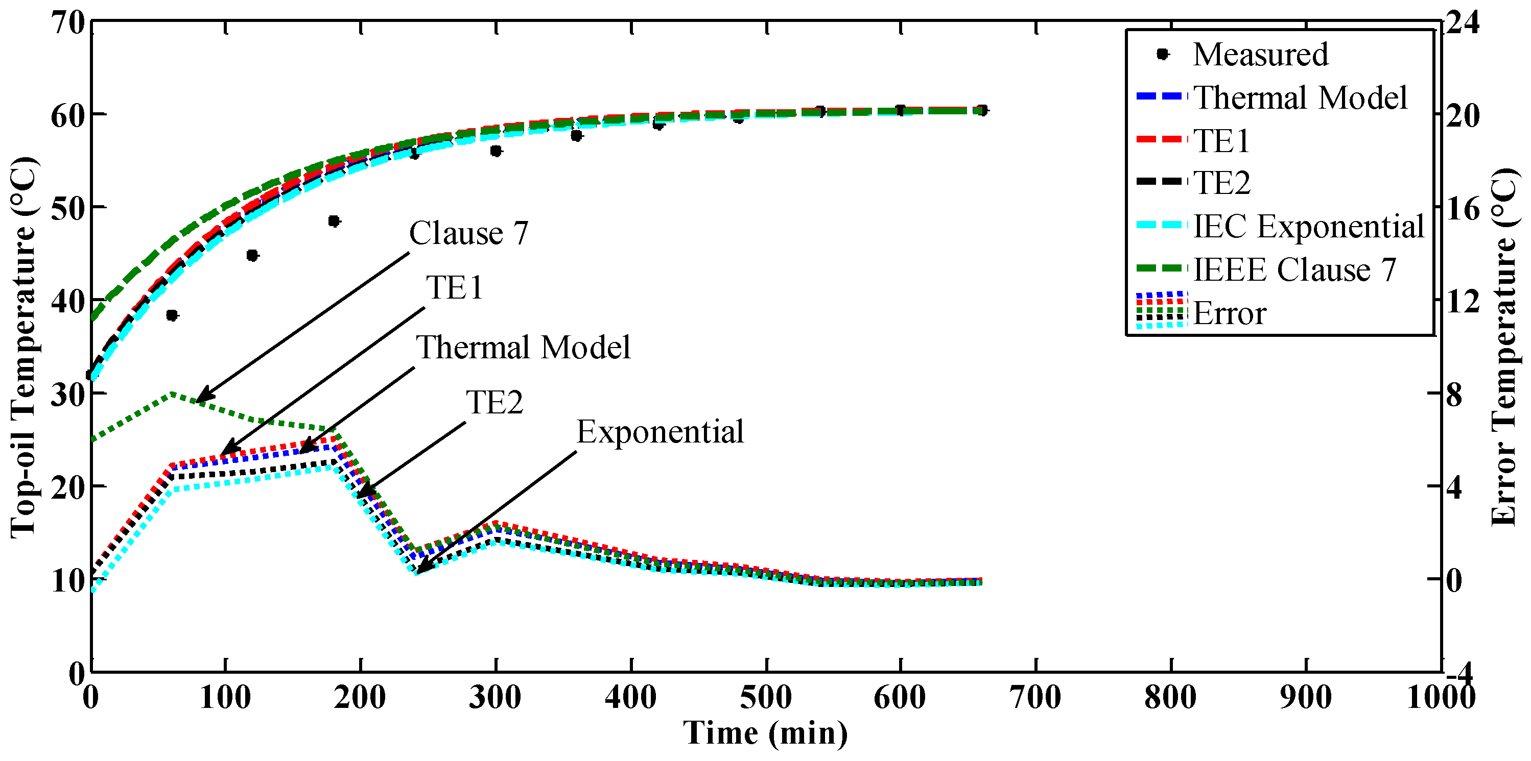
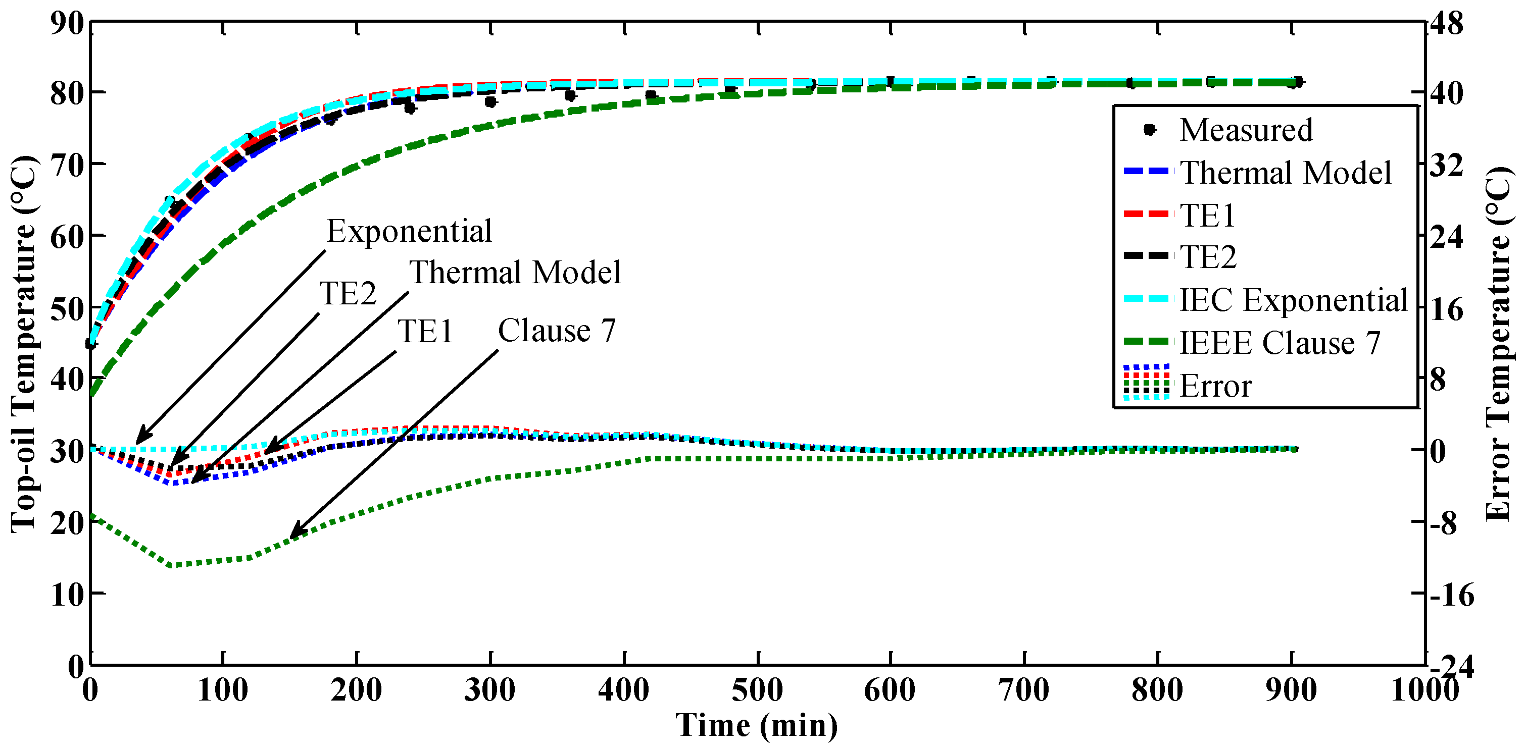
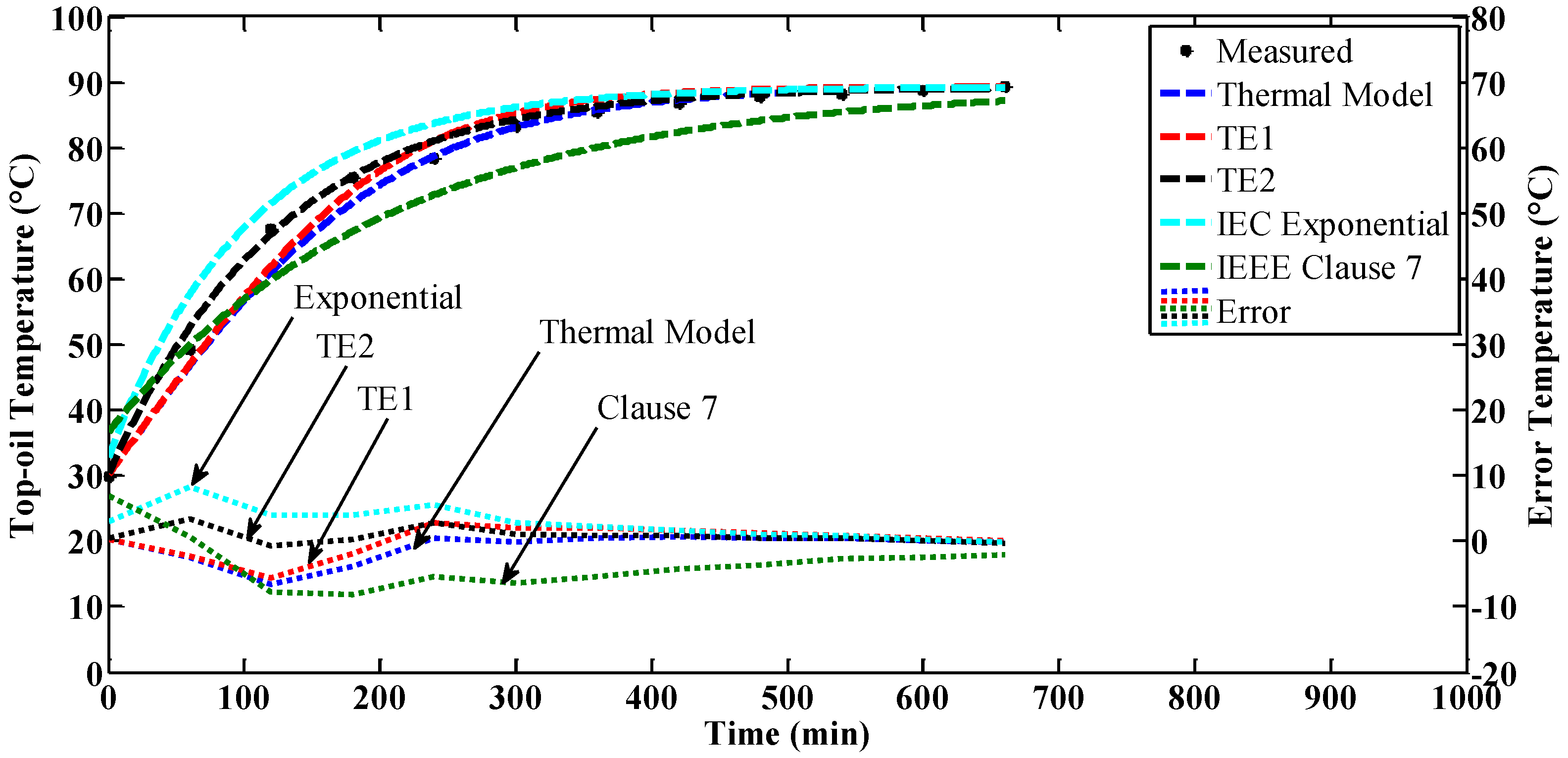
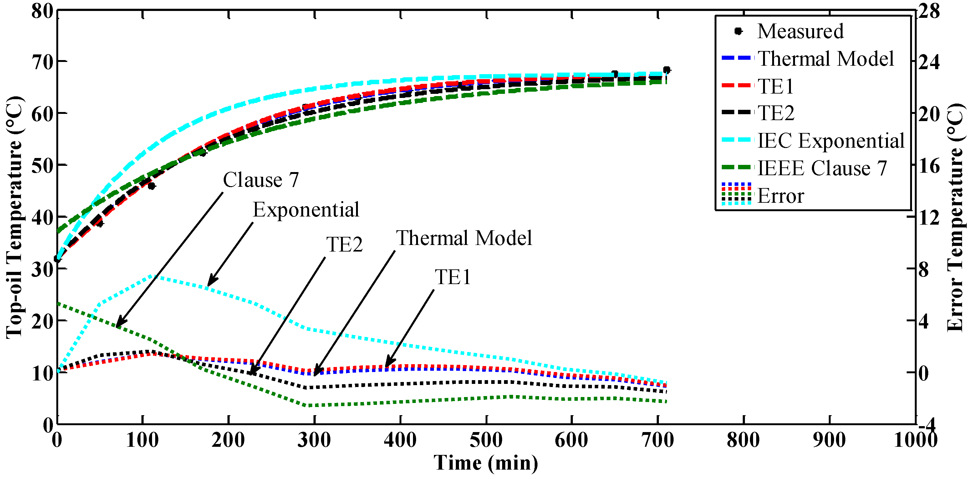
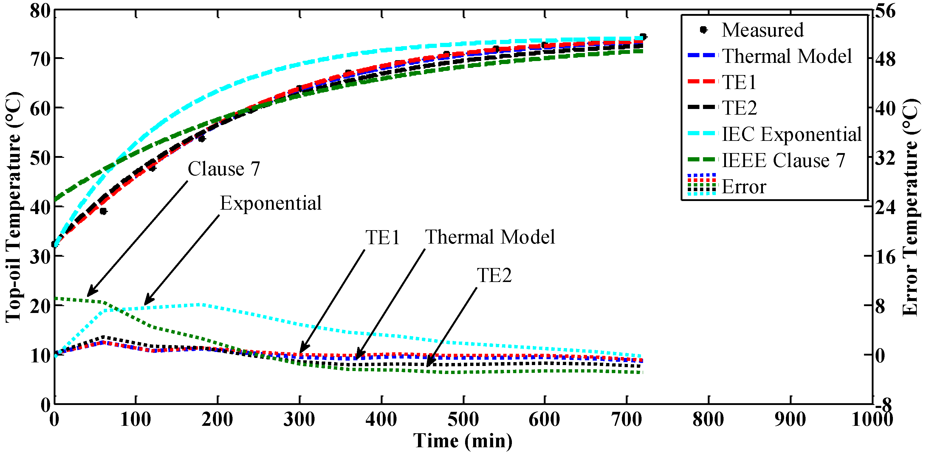
4.1. Constant Loading

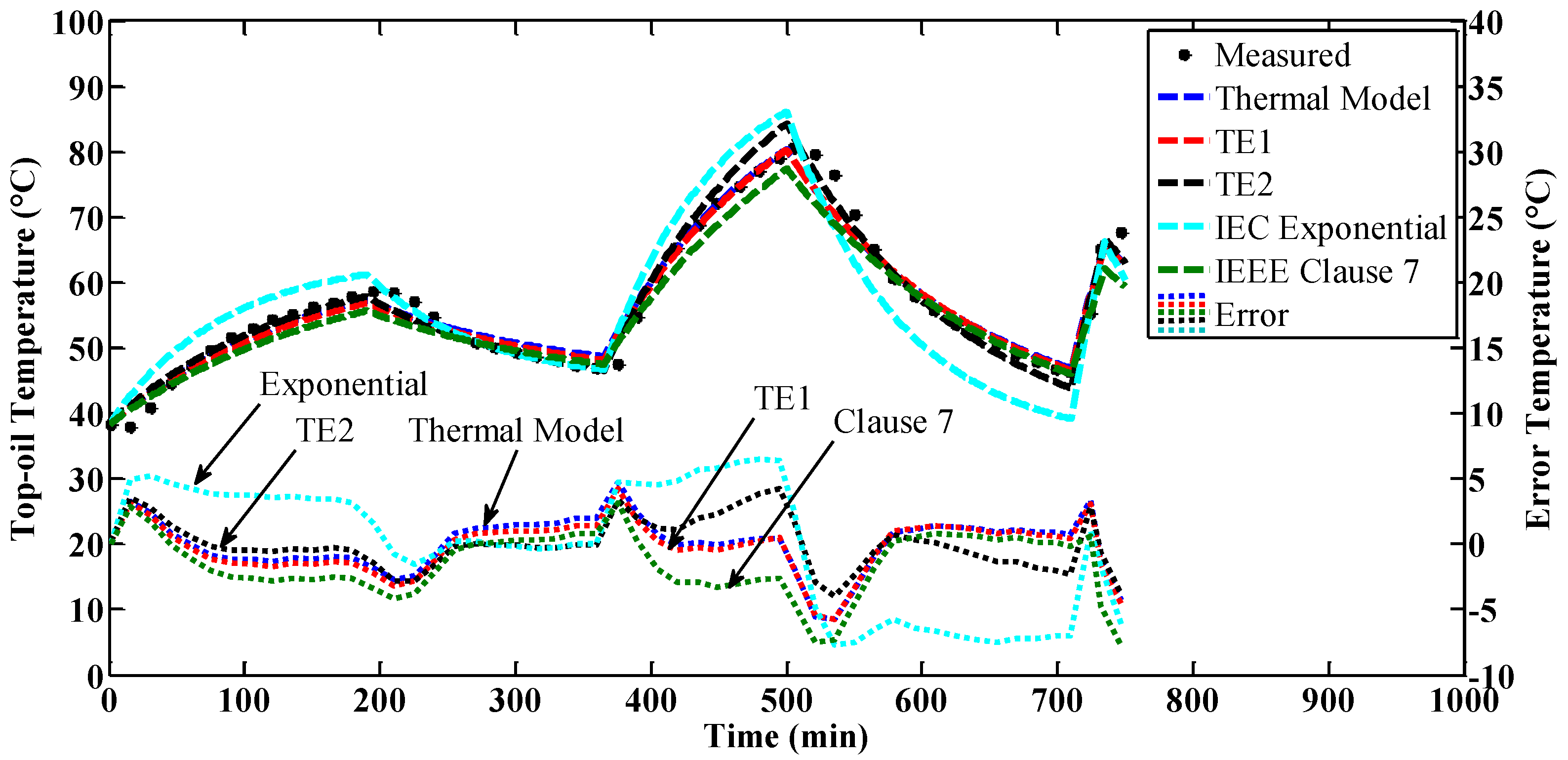
The comparison between the TOT thermal model and the existing TOT Thermal-Electrical, Exponential (IEC 60076-7) and Clause 7 (IEEE C57.91-1995) models can be seen in Figure 7, Figure 8, Figure 9, Figure 10, Figure 11, Figure 12 and Figure 13. For TX1, the simulated TOT for all thermal models overshoot during the first 300 min of the temperature rise test as seen in Figure 7. The maximum errors for the TOT thermal, TE1, TE2, Exponential, and Clause 7 models are 5.65 °C, 5.98 °C, 5.03 °C, 4.79 °C, and 7.92 °C. Meanwhile, the RMS errors are 2.72 °C, 2.89 °C, 2.41 °C, 2.23 °C, and 4.02 °C. The measured TOT for TX2 is well represented by the TOT thermal, TE1, TE2, and Exponential models, as shown in Figure 8. However, the simulated TOT based on the Clause 7 model is lower than the measured TOT during the first 300 min of the temperature rise test. The maximum errors of the TOT thermal, TE1, TE2, Exponential, and Clause 7 models are 3.72 °C, 2.77 °C, 2.09 °C, 2.15 °C, and 12.92 °C, while the RMS errors are 1.34 °C, 1.33 °C, 0.97 °C, 1.03 °C, and 5.33 °C. The simulated TOT based on TE2 and Exponential models are much closer to the measured TOT than the TOT thermal, TE1, and Clause 7 models for TX3. The same pattern is observed for TX4 and it is expected since both transformers have the same design, except for its cooling modes. For TX3, the maximum errors for TOT thermal, TE1, TE2, Exponential, and Clause 7 models are 6.53 °C, 6.32 °C, 0.91 °C, 3.30 °C, and 8.25 °C, while for TX4, the values are 6.66 °C, 5.71 °C, 3.35 °C, 8.37 °C, and 8.24 °C. On the other hand, the RMS errors of TX3 for the TOT thermal, TE1, TE2, Exponential, and Clause 7 models are 2.76 °C, 2.49 °C, 0.56 °C, 2 °C, and 5.17 °C, while for TX4, the values are 2.36 °C, 2.28 °C, 1.38 °C, 3.61 °C, and 5.20 °C, respectively.

The TOT thermal, TE1, and TE2 models can represent the measured TOT for TX5 quite well as compared with the Exponential and Clause 7 models. The maximum and RMS errors for TOT thermal model are 1.43 °C and 0.67 °C. For TE1, TE2, Exponential and Clause 7 models, the maximum errors are 1.42 °C, 1.64 °C, 7.44 °C, and 5.30 °C, while the RMS errors are 0.70 °C, 1.04 °C, 3.72 °C, and 2.65 °C, respectively. The same pattern is observed for TX6 and TX7, except the simulated TOT based on the Clause 7 model for TX7 is lower than the measured TOT during the initial stage of the temperature rise test. On the other hand, the simulated TOT based on the Exponential model is higher than the measured TOT during the first 500 min. The maximum errors for TX6 for TOT thermal, TE1, TE2, Exponential, and Clause 7 models are 2.01 °C, 1.98 °C, 2.85 °C, 8.04 °C, and 9.04 °C, while for TX7, the values are 2.14 °C, 2.03 °C, 2 °C, 6.67 °C, and 6.84 °C. Meanwhile, the RMS errors of TX6 for the TOT thermal, TE1, TE2, Exponential, and Clause 7 models are 0.81 °C, 0.72 °C, 1.54 °C, 4.54 °C, and 4.24 °C, while for TX7, the values are 0.95 °C, 0.88 °C, 1 °C, 3.39 °C, and 4.33 °C, respectively.

4.2. Step Loading

The performance of the TOT thermal model is also tested on step loading of TX8 as shown in Figure 14. The simulated TOT based on TOT thermal and TE1 models are quite close to measured TOT. The simulated TOT based on both TE2 and Exponential models slightly overshoot once the loading increases from 0 to 1.0 p.u. and 0.6 to 1.5 p.u. On the other hand, the simulated TOT based on the Clause 7 model is slightly lower than measured TOT during the same loading period. A significant deviation between simulated TOT based on Exponential model and measured TOT is found once the loading decreases from 1.5 to 0.3 p.u. The maximum errors for the TOT thermal, TE1, TE2, Exponential, and Clause 7 models are 5.77 °C, 5.70 °C, 4.22 °C, 7.70 °C, and 7.76 °C, while the RMS errors are 2.02 °C, 2 °C, 1.91 °C, 4.78 °C, and 2.84 °C, respectively.

4.3. Discussions

Under constant loadings of seven transformers, the highest maximum and RMS errors for the TOT thermal model are 6.66 °C and 2.76 °C, which are lower than Exponential and Clause 7 models where the highest maximum errors are 8.37 °C and 12.92 °C while the highest RMS error are 4.54 °C and 5.33 °C, respectively. The performance of TE1 and TE2 models are slightly better than TOT thermal model where the highest maximum errors are 6.32 °C and 5.03 °C while the highest RMS error are 2.89 °C and 2.41 °C. Meanwhile, under step loading, the TOT thermal model performs better than Exponential and Clause 7 models, and comparable with TE1 and TE2 models. The TE1 model is able to represent the TOT better than the TOT thermal model owing to its comprehensive consideration on the viscosity. However, due to the minimal information requirement by the TOT thermal model, the performance could be considered as reasonable as alternative approach to determine the TOT of transformers. Furthermore, the TOT thermal model is able to evaluate transformers with different cooling modes since the oil time constant, ${\tau }_{oil}$ is calculated according to the respective cooling modes.

5. Conclusions

Based on the proposed pathway of the energy transfer concept and thermal-electrical analogy through utilization of the nonlinear thermal resistance and lumped capacitance method, an alternative approach to determine the TOT is developed. The key component of the TOT thermal model is the alternative approximation of the convection coefficient, h, proposed based on heat transfer theory that eliminates the requirement of the viscosity. The TOT thermal model was tested on seven transformers with either ONAN or ONAF cooling modes. Based on the case study, the TOT thermal model can represent the measured TOT quite well where the highest maximum and RMS errors are 6.66 °C and 2.76 °C, respectively. Under step loading, the performance of TOT thermal model is comparable with other types of thermal models where the simulated TOT is quite close to measured TOT and the maximum and RMS errors are 5.77 °C and 2.02 °C. Overall, the performance of the TOT thermal model is comparable with the TE1 and TE2 models and better than the Exponential and Clause 7 models.

References

1. Standard, I. 60076-7 Power Transformer—Part 7:‘Loading Guide for Oil-Immersed Power Transformers’; IEC: Geneva, Switzerland, 2005. [Google Scholar]
2. IEEE. IEEE Guide for Loading Mineral-Oil-Immersed Transformers; IEEE Std C57.91-1995; IEEE: Piscataway Township, NJ, USA, 1996. [Google Scholar]
3. Swift, G.; Molinski, T.S.; Lehn, W. A Fundamental Approach to Transformer Thermal Modeling. I. Theory and Equivalent Circuit. IEEE Trans. Power Deliv. 2001, 16, 171–175. [Google Scholar] [CrossRef]
4. Swift, G.; Molinski, T.S.; Bray, R.; Menzies, R. A fundamental approach to transformer thermal modeling. II. Field verification. IEEE Trans. Power Deliv. 2001, 16, 176–180. [Google Scholar] [CrossRef]
5. Susa, D.; Lehtonen, M.; Nordman, H. Dynamic thermal modelling of power transformers. IEEE Trans. Power Deliv. 2005, 20, 197–204. [Google Scholar] [CrossRef]
6. Susa, D.; Lehtonen, M. Dynamic thermal modeling of power transformers: Further development-part I. IEEE Trans. Power Deliv. 2006, 21, 1961–1970. [Google Scholar] [CrossRef]
7. Susa, D.; Lehtonen, M. Dynamic thermal modeling of power transformers: Further development-part II. IEEE Trans. Power Deliv. 2006, 21, 1971–1980. [Google Scholar] [CrossRef]
8. Chen, W.G.; Pan, C.; Yun, Y.X. Power transformer top-oil temperature model based on thermal–electric analogy theory. Eur. Trans. Electr. Power 2009, 19, 341–354. [Google Scholar]
9. Iskender, I.; Mamizadeh, A. An improved nonlinear thermal model for MV/LV prefabricated oil-immersed power transformer substations. Electr. Eng. 2011, 93, 9–22. [Google Scholar] [CrossRef]
10. Mamizadeh, A.; Iskender, I. Analyzing and Comparing Thermal Models of Indoor and Outdoor Oil-Immersed Power Transformers. In Proceedings of the IEEE Bucharest Power Tech, Bucharest, Romania, 28 June–2 July 2009; pp. 1–8. [Google Scholar]
11. Su, X.; Chen, W.; Pan, C.; Zhou, Q.; Teng, L. A simple thermal model of transformer hot spot temperature based on thermal-electrical analogy. In Proceedings of the International Conference on High Voltage Engineering and Application (ICHVE), Shanghai, China, 17–20 September 2012; pp. 492–495. [Google Scholar]
12. Ben-gang, W.; Chen-zhao, F.; Hong-lei, L.; Ke-jun, L.; Yong-liang, L. The improved thermal-circuit model for hot-spot temperature calculation of oil-immersed power transformers. In Proceedings of the IEEE Information Technology, Networking, Electronic and Automation Control Conference, Chongqing, China, 20–22 May 2016; pp. 809–813. [Google Scholar]
13. Zhou, L.; Wu, G.; Yu, J.; Zhang, X. Thermal overshoot analysis for hot-spot temperature rise of transformer. IEEE Trans. Dielectr. Electr. Insul. 2007, 14, 1316–1322. [Google Scholar] [CrossRef]
14. Li, R.; Yi, Y.Y. Study on Prediction of Top Oil Temperature for Transformers Based on Bayesian Network Model. In Proceedings of the MATEC Web of Conferences, Hong Kong, China, 11–12 June 2016. [Google Scholar]
15. Yi, Y.Y.; Li, R. Application of Gray Neural Network Combined Model in Transformer Top-oil Temperature Forecasting. In Proceedings of the MATEC Web of Conferences, Hong Kong, China, 11–12 June 2016. [Google Scholar]
16. He, Q.; Si, J.; Tylavsky, D.J. Prediction of top-oil temperature for transformers using neural networks. IEEE Trans. Power Deliv. 2000, 15, 1205–1211. [Google Scholar] [CrossRef]
17. Taghikhani, M.A. Power transformer top oil temperature estimation with GA and PSO methods. Energy Power Eng. 2012, 4, 41–46. [Google Scholar] [CrossRef]
18. Assunção, T.; Silvino, J.; Resende, P. Transformer top-oil temperature modeling and simulation. Trans. Eng. Comput. Technol. 2006, 15, 240–245. [Google Scholar]
19. Radakovic, Z.; Feser, K. A new method for the calculation of the hot-spot temperature in power transformers with ONAN cooling. IEEE Trans. Power Deliv. 2003, 18, 1284–1292. [Google Scholar] [CrossRef]
20. Tang, W.; Wu, Q.; Richardson, Z. Equivalent heat circuit based power transformer thermal model. IEEE Proc. Electr. Power Appl. 2002, 149, 87–92. [Google Scholar] [CrossRef]
21. Tang, W.; Wu, Q.; Richardson, Z. A simplified transformer thermal model based on thermal-electric analogy. IEEE Trans. Power Deliv. 2004, 19, 1112–1119. [Google Scholar] [CrossRef]
22. Cui, Y.; Ma, H.; Saha, T.; Ekanayake, C.; Martin, D. Moisture-Dependent Thermal Modelling of Power Transformer. IEEE Trans. Power Deliv. 2016, 31, 2140–2150. [Google Scholar] [CrossRef]
23. Bergman, T.L.; Incropera, F.P.; Lavine, A.S. Fundamentals of Heat and Mass Transfer; John Wiley & Sons: New York, NY, USA, 2011. [Google Scholar]
24. Perez, J. Fundamental principles of transformer thermal loading and protection. In Proceedings of the 63rd Annual Conference for Protective Relay Engineers, College Station, TX, USA, 29 March–1 April 2010; pp. 1–14. [Google Scholar]
25. Xiao, B.; Wang, W.; Fan, J.; Chen, H.; Hu, X.; Zhao, D.; Zhang, X.; Ren, W. Optimization of the fractal-like architecture of porous fibrous materials related to permeability, diffusivity and thermal conductivity. Fractals 2017. [CrossRef]
26. Xiao, B.; Chen, H.; Xiao, S.; Cai, J. Research on relative permeability of nanofibers with capillary pressure effect by means of Fractal-Monte Carlo technique. J. Nanosci. Nanotechnol. 2017, 17, 6811–6817. [Google Scholar] [CrossRef]
27. Incropera, F.; DeWitt, D. Fundamentals of Heat and Mass Transfer; Wiley: New York, NY, USA, 1996. [Google Scholar]
Figure 1. Pathway of energy in transformers.
Energies 10 01843 g001
Figure 2. Thermal resistance equivalent circuit.
Energies 10 01843 g002
Figure 3. Thermal resistance equivalent circuit with heat source.
Energies 10 01843 g003
Figure 4. Thermal resistance equivalent circuit with a heat source and without the thermal resistance of the tank/radiator.
Energies 10 01843 g004
Figure 5. Thermal resistance equivalent circuit with lumped capacitance.
Energies 10 01843 g005
Figure 6. Thermal-electrical analogy circuit: (a) hot-spot temperature; and (b) top-oil temperature.
Energies 10 01843 g006
Figure 7. TOT based on different thermal models for TX1.
Energies 10 01843 g007
Figure 8. TOT based on different thermal models for TX2.
Energies 10 01843 g008
Figure 9. TOT based on different thermal models for TX3.
Energies 10 01843 g009
Figure 10. TOT based on different thermal models for TX4.
Energies 10 01843 g010
Figure 11. TOT based on different thermal models for TX5.
Energies 10 01843 g011
Figure 12. TOT based on different thermal models for TX6.
Energies 10 01843 g012
Figure 13. TOT based on different thermal models for TX7.
Energies 10 01843 g013
Figure 14. TOT based on different thermal models for TX8.
Energies 10 01843 g014