An Adaptive Model Predictive Load Frequency Control Method for Multi-Area Interconnected Power Systems with Photovoltaic Generations

Abstract

As the penetration level of renewable distributed generations such as wind turbine generator and photovoltaic stations increases, the load frequency control issue of a multi-area interconnected power system becomes more challenging. This paper presents an adaptive model predictive load frequency control method for a multi-area interconnected power system with photovoltaic generation by considering some nonlinear features such as a dead band for governor and generation rate constraint for steam turbine. The dynamic characteristic of this system is formulated as a discrete-time state space model firstly. Then, the predictive dynamic model is obtained by introducing an expanded state vector, and rolling optimization of control signal is implemented based on a cost function by minimizing the weighted sum of square predicted errors and square future control values. The simulation results on a typical two-area power system consisting of photovoltaic and thermal generator have demonstrated the superiority of the proposed model predictive control method to these state-of-the-art control techniques such as firefly algorithm, genetic algorithm, and population extremal optimization-based proportional-integral control methods in cases of normal conditions, load disturbance and parameters uncertainty.

1. Introduction

Load-frequency control (LFC) issue in a multi-area interconnected power system is essentially to design an effective and efficient controller to match the total generations with the total load demand and the corresponding system losses. In other words, the main objective of LFC is to minimize the frequency deviations of each area and tie-line power flows between neighboring control areas subjecting to some pre-specified tolerances when load demands fluctuate or resonance attack [1,2]. Over the past four decades, a variety of great achievements have been made for the LFC issueof traditional power systems. For example, as the most popular control technique, proportional-integral-derivative (PID) controller and its various variations have been widely applied to the LFC issue [3,4,5,6,7,8]. Moreover, some researchers have paid more attention to the advanced control theories based LFC methods recently, such as robust control theories [9], model predictive control [10,11,12,13,14], sliding mode control [15,16], neural network control [17], internal model control [18], and differential games [19]. It should be noted that there are different evolutionary algorithms based PID or proportional-integral (PI) control methods for the LFC issue of multi-area power systems. For example, genetic algorithm 5,6, hybrid particle swarm optimization [20], differential evolution [21,22], imperial competitive algorithm [23], firefly algorithm [24], non-dominated sorting genetic algorithm-II (NSGA-II) [8], multi-objective optimization using weighted sum artificial bee colony algorithm [7], and a evolutionary many-objective optimization algorithm with clustering-based selection called EMyO/C [25] have been utilized to tune PID or PI controllers for the LFC issue.

As increased penetration level of renewable distributed generations such as wind turbine generator and photovoltaic stations, these renewable generations affects the LFC problem of multi-area power system tremendously. The effects of wind turbine generators on LFC issues of multi-area power systems have been discussed recently [26,27,28,29,30,31]. Unfortunately, only few research works contribute to the LFC problem of multi-area power system with photovoltaic (PV) generations. Abd-Elazim and Ali [32] proposed firefly algorithm (FA)-based PI controllers for LFC of a two-area power system composing of a photovoltaic (PV) system and a thermal generator, and its effectiveness is demonstrated by comparing the performance with genetic algorithm (GA)-based PI control method for this system under load disturbance and parameters uncertainty conditions. However, the nonlinear features such as the dead band (DB) for governor and generation rate constraint (GRC) for steam turbine have not been considered in the recently reported work [32]. By taking into account these nonlinear features, how to further improve the LFC performance of a multi-area power system with PV generation especially under dynamical loads fluctuations is still a challenging issue.

On the other hand, model predictive control (MPC) ranks second after PID as the most widely-applied control methods in industry [33,34]. Compared to PID controller, MPC has some significant advantages including fast response and stronger robustness against load disturbance and parameters uncertainty. Especially, one prominent characteristics of MPC is predicting the future behavior of the desired control variables based on a minimization cost function until a predefined horizon in time. With the rapid development of high-speed microprocessors, MPC has been applied increasingly to “fast-process” systems such as power converters and power systems in the past decade [10,11,12,13,14,35,36,37,38,39,40,41]. However, to the best of the authors’ knowledge, MPC has never applied to the optimal LFC issue of multi-area power system with PV generations.

Motivated by the above analysis, we propose an adaptive model predictive load frequency control method for a multi-area interconnected power system with PV generation. The key idea behind the proposed method is formulating the dynamic load frequency control issue as a discrete-time state space model, obtaining the predictive dynamic model by introducing an expanded state vector, and rolling optimization of control output signal based on a cost function by minimizing the weighted sum of square predicted errors and square future control values. The simulation results on a typical two-area power system consisting of PV and thermal generator will demonstrate the superiority of the proposed MPC method to these existing evolutionary algorithms-based PI control methods such as FA-PI [32] GA-PI [32], and population extremal optimization-based PI denoted as PEO-PI [42,43] in cases of normal condition, load disturbance and parameters uncertainty.

The main contribution of this work is described as follows:

(1)

To the best of the authors’ knowledge, an extended MPC method with an extended state vector is proposed firstly for the optimal LFC issue of a multi-area interconnected power system with PV generation.

(2)

Compared with two state-of-the-art control methods reported in [32], this proposed MPC method considers some nonlinear features such as DB and GRC in a thermal system.

(3)

In cases of load disturbance and parameters uncertainty, the proposed MPC method can improve the control performance of a multi-area interconnected power system with PV generation compared with these state-of-the-art control methods [32,42].

The rest of this paper is organized as follows. Section 2 presents the dynamic model of a two-area power system consisting of PV and thermal generator. In Section 3, an adaptive MPC based LFC method is proposed for a multi-area power system with PV generation. The comparative studies on a typical test system in cases of normal condition, load disturbance and parameters uncertainty are provided in Section 4. Finally, we give the conclusions and open problems in Section 5.

2. System Model

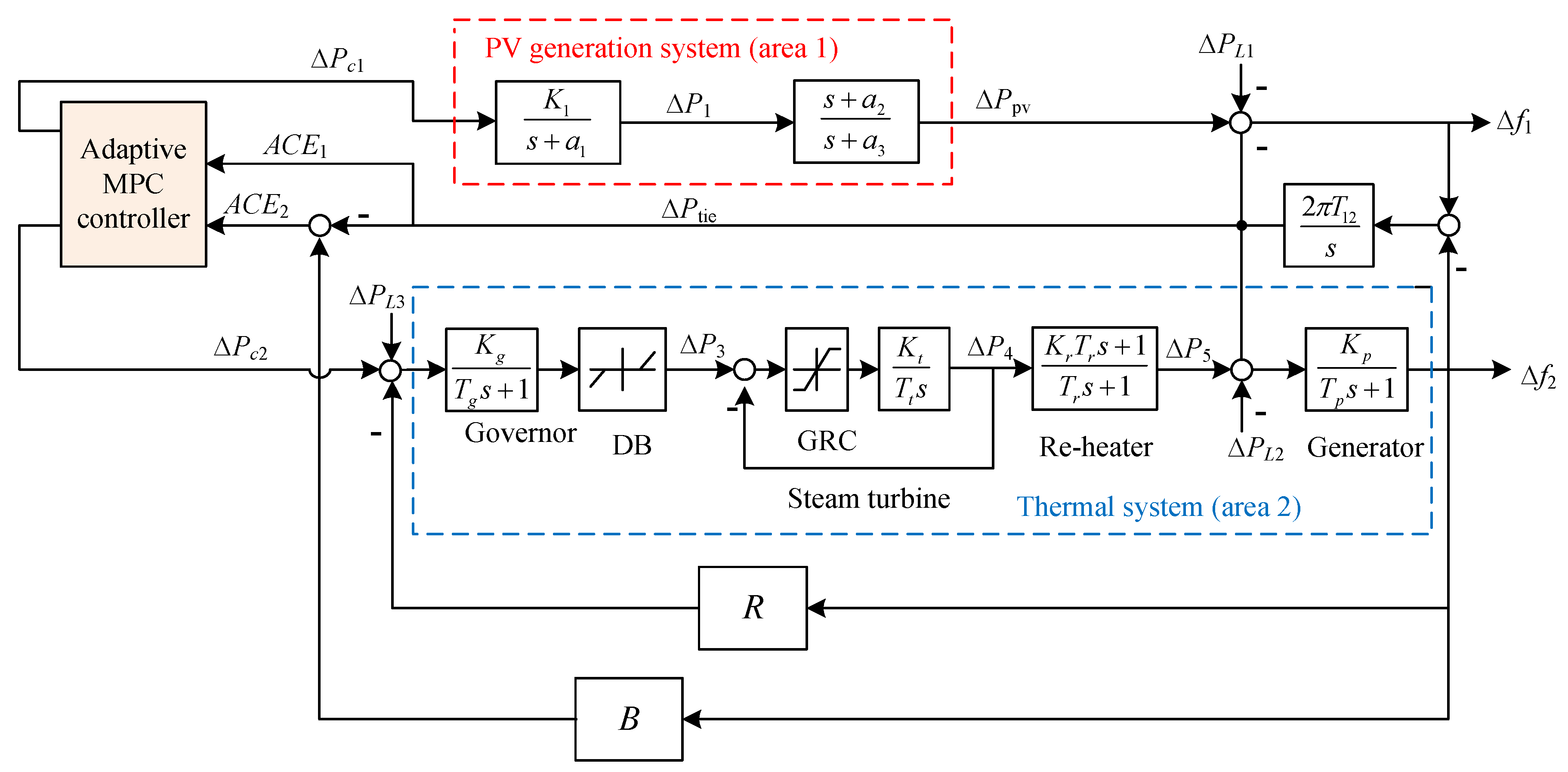
2.1. Small-Signal Model

Figure 1 shows the block diagram of a two-area interconnected power system composed of a PV system(area 1) and a thermal system (area 2) [32]. It should be noted that there are some important nonlinear features in a thermal system such as the dead band (DB) for governor and generation rate constraint (GRC) for steam turbine, but these nonlinear features has never been considered in the recently reported work [32]. In order to make up this defect, this paper introduces these nonlinearities including DB and GRC in a thermal system [44,45].

For area 1, the equivalent transfer function of the PV system consisting of the PV panel, maximum power point tracking (MPPT), inverter and filter is described by the following equation [32]:

$$G_{PV}(s)=\frac{K_1}{s+a_1}\frac{s+a_2}{s+a_3},$$

(1)

whereK₁ is the gain of PV system, a₁ and a₃ are the negative values of poles, and a₂ is the negative value of zero in transfer function.

The area control error (ACE) of area 1 is defined as follows [32]:

$$AC{E}_1(s)=\Delta P_{\mathrm{tie}}(s)=\frac{2\pi T_{12}\left(\Delta f_1(s)-\Delta f_2(s)\right)}{s},$$

(2)

where ΔP_tie(s) is the change of tie line power (p.u.), Δf₁ and Δf₂ are the frequency deviation of area 1 and area 2, respectively, T₁₂ is the synchronizing coefficient of tie line between area 1 and area 2.

Area 2 is a thermal system that consists of a governor, steam turbine, re-heater, and generator. The transfer function of governor G_go(s) is as follows [32]:

$$G_{go}(s)=\frac{K_g}{T_{g}s+1},$$

(3)

where K_g is the gain of governor, and T_g is the first order inertial time constant of governor.

The transfer function of steam turbine G_t(s) is as follows [32]:

$$G_t(s)=\frac{K_t}{T_{t}s+1},$$

(4)

where K_t is the gain of governor, and T_t is the first order inertial time constant of steam turbine.

The transfer function of re-heater G_r(s) is as follows [32]:

$$G_r(s)=\frac{K_r{T}_{r}s+1}{T_{r}s+1},$$

(5)

where K_r is the p.u. megawatt rating of high pressure stage, and T_r is the time constant of re-heater.

The transfer function of generator G_ge(s) is as follows [32]:

$$G_{ge}(s)=\frac{K_p}{T_{p}s+1},$$

(6)

where K_p is the gain of generator, and T_p is the first order inertial time constant of generator.

For area 2, the ACE is defined as follows [32]:

$$AC{E}_2(s)=-\Delta P_{\mathrm{tie}}(s)+B\Delta f_2(s),$$

(7)

where B is the biasing factor in p.u. MW/Hz.

The dynamic characteristics of the power and frequency changes in this two-area power system is reformulated as the following equations:

$$\Delta {\dot{P}}_1(t)=-a_1\Delta P_1(t)+K_1\Delta P_{c1}(t),$$

(8)

$$\Delta {\dot{P}}_{\mathrm{pv}}(t)=(a_2-a_1)\Delta P_1(t)-a_3\Delta P_{\mathrm{pv}}(t)+K_1\Delta P_{c1}(t),$$

(9)

$$\Delta {\dot{P}}_{\mathrm{tie}}(t)=2\pi T_{12}\left(\Delta P_{\mathrm{pv}}(t)-\Delta P_{\mathrm{tie}}(t)-\Delta f_2(t)-\Delta P_{L1}(t)\right),$$

(10)

$$\Delta {\dot{f}}_2(t)=\frac{K_P}{T_P}\Delta P_{\mathrm{tie}}(t)-\frac{1}{T_P}\Delta f_2(t)+\frac{K_P}{T_P}\Delta P_5(t)-\frac{K_P}{T_P}\Delta P_{L2}(t),$$

(11)

$$\Delta {\dot{P}}_3(t)=-\frac{R}{T_g}\Delta f_2(t)-\frac{1}{T_g}\Delta P_3(t)+\frac{1}{T_g}\Delta P_{c2}(t)+\frac{1}{T_g}\Delta P_{L3}(t),$$

(12)

$$\Delta {\dot{P}}_4(t)=\frac{1}{T_t}\Delta P_3(t)-\frac{1}{T_t}\Delta P_4(t),$$

(13)

$$\Delta {\dot{P}}_5(t)=\frac{K_r{T}_r}{T_t{T}_r}\Delta P_3(t)+(\frac{1}{T_r}-\frac{K_r{T}_r}{T_t{T}_r})\Delta P_4(t)-\frac{1}{T_r}\Delta P_5(t),$$

(14)

$$AC{E}_1(t)=\Delta P_{\mathrm{tie}}(t),$$

(15)

$$AC{E}_2(t)=-\Delta P_{\mathrm{tie}}(t)+B\Delta f_2(t),$$

(16)

where ΔP₁(t) is the intermediate power change of PV, ΔP_pv(t) is power change of PV, ΔP_tie(t) is the total tie-line power change in this system, Δf₁(t) and Δf₂(t) are the frequency deviations of area 1 and area2, respectively, ΔP₃(t), ΔP₄(t), and ΔP₅(t)are the power change of governor, steam turbine, and re-heater, respectively, ΔP_c1(t) and ΔP_c2(t) are the control action of area1 and area2, respectively. ΔP_L1(t), ΔP_L2(t), and ΔP_L3(t)are the load changes, B is frequency bias factor, and R is the regulation constant (Hz/p.u.MW).

2.2. State-Space Model

Define the state vector x(t), the control vector u(t), the disturbance vector u_I(t) and system output vector y(t) as: x(t) = [ΔP₁(t) ΔP_pv(t) ΔP_tie(t) Δf₂(t) ΔP₃(t) ΔP₄(t) ΔP₅(t)]^T, u(t) = [ΔP_c1(t) ΔP_c2(t)]^T, u_I(t) = [ΔP_L1(t) ΔP_L2(t) ΔP_L3(t)]^T, and y(t) = [ACE₁(t) ACE₂(t)]^T.

The state space model of the aforementioned two-area interconnected power system with PV generation is described as the following equations:

$$\begin{array}{l}\frac{dx(t)}{dt}=Ax(t)+{\rm B}u(t)+B_I{u}_I(t)\hfill \\ y(t)=Cx(t)\hfill \end{array},$$

(17)

where A, B, B_I and C are parameter matrices of x(t), u(t), u_I(t), and y(t), respectively.

$$\begin{array}{cc}A& =\left[\begin{array}{ccccccc}-a_1& 0& 0& 0& 0& 0& 0\\ a_2-a_1& -a_3& 0& 0& 0& 0& 0\\ 0& T_{12}& -2\pi T_{12}& -2\pi T_{12}& 0& 0& 0\\ 0& 0& \frac{K_p}{T_p}& -\frac{1}{T_p}& 0& 0& \frac{K_p}{T_p}\\ 0& 0& 0& -\frac{R}{T_g}& -\frac{1}{T_g}& 0& 0\\ 0& 0& 0& 0& \frac{1}{T_t}& -\frac{1}{T_t}& 0\\ 0& 0& 0& 0& \frac{K_r\times T_r}{T_t\times T_r}& \frac{1}{T_r}-\frac{K_r\times T_r}{T_t\times T_r}& -\frac{1}{T_r}\end{array}\right],\hfill \\ B& =\left[\begin{array}{cc}{K}_1& 0\\ K_1& 0\\ 0& 0\\ 0& 0\\ 0& \frac{1}{T_g}\\ 0& 0\\ 0& 0\end{array}\right]B_I=\left[\begin{array}{ccc}0& 0& 0\\ 0& 0& 0\\ -2\pi T_{12}& 0& 0\\ 0& -\frac{K_p}{T_p}& 0\\ 0& 0& \frac{1}{T_g}\\ 0& 0& 0\\ 0& 0& 0\end{array}\right],C=\left[\begin{array}{ccccccc}0& 0& 1& 0& 0& 0& 0\\ 0& 0& -1& B& 0& 0& 0\end{array}\right].\hfill \end{array}$$

By discretization with sampling time T_s, the discrete-time state space model of (17) is obtained by the following equation:

$$\begin{array}{l}x(k+1)=A_{d}x(k)+B_{d}u(k)+B_{Id}{u}_I(k)\hfill \\ y(k)=Cx(k)\hfill \end{array},$$

(18)

where x(k+1), x(k), u(k), u_I(k), and y(k) are the discrete-time forms of dx(t)/dt, x(t), u(t), u_I(t), and y(t), respectively, $A_d=e^{A{T}_s}$, $B_d={\displaystyle {\int }_0^{T_s}{e}^{At}Bdt}$, $B_{Id}={\displaystyle {\int }_0^{T_s}{e}^{At}{B}_{I}dt}$.

The incremental form of Equation (18) is defined as follows:

$$\begin{array}{l}\Delta x(k+1)=A_d\Delta x(k)+B_d\Delta u(k)+B_{Id}\Delta u_I(k)\hfill \\ \Delta y(k)=C\Delta x(k)\hfill \end{array}$$

(19)

where Δx(k+1), Δx(k), Δu(k), Δu_I(k), and Δy(k) are the incremental forms of x(k+1), x(k), u(k), u_I(k), and y(k), respectively.

3. The Proposed Method

In this section, we present an adaptive model predictive load frequency control method for a multi-area interconnected power system with PV generation. The key idea behind the proposed method is obtaining the dynamic predictive model by introducing an expanded state vector, and rolling optimization of control signal vectors based on a cost function by minimizing the weighted sum of square predicted errors and square future control values.

By defining an extend state vector Z(k) = (Δx(k) y(k− 1))^T, the following expanded discrete-time state space model is reformulated according to the Equations (18) and (19):

$$\begin{array}{l}Z(k+1)=GZ(k)+H\Delta u(k)+H_I\Delta u_I(k)\hfill \\ y(k)=C_{z}Z(k)\hfill \end{array}$$

(20)

where $G={\left(\begin{array}{cc}{A}_d& 0_{N_x\times N_y}\\ C& E_{N_y}\end{array}\right)}_{(N_x+N_y)\times (N_x+N_y)}$, $H={\left(\begin{array}{c}{B}_d\\ 0_{N_y\times N_u}\end{array}\right)}_{(N_x+N_y)\times N_u}$, $H_I={\left(\begin{array}{c}{B}_{Id}\\ 0_{N_y\times N_{uI}}\end{array}\right)}_{(N_x+N_y)\times N_{uI}}$, $C_z={\left(\begin{array}{cc}C& E_{N_y}\end{array}\right)}_{N_y\times (N_x+N_y)}$, $E_{N_y}$ is an identity matrix with N_y rows and N_y columns, $0_{N_x\times N_y}$ is a zero matrix with N_x rows and N_y columns, N_x, N_y, N_u and N_uI are the states number of x(t), y(t), u(t) and u_I(t), respectively.

The predictive output value y(k+p|k) at k-th sample time is calculated as follows:

$$y\left(k+p|k\right)=C_z{G}^{p}Z(k)+{\displaystyle \sum _{j=1}^p{C}_z{G}^{p-j}H\Delta u(k+j-1)}+{\displaystyle \sum _{j=1}^p{C}_z{G}^{p-j}{H}_I\Delta u_I(k+j-1)},p=1,2,\cdots ,P,$$

(21)

where P is prediction horizon, and M is the control horizon.

The predictive output vector Y_P(k) is evaluated as follows:

$$Y_P(k)=\varphi Z(k)+\psi \Delta U(k)+{\psi }_I\Delta U_I(k),$$

(22)

where each vector is defined as follows:

$$\begin{gathered} Y_P(k)={\left(\begin{array}{c}y\left(k+1|k\right)\\ \dots \\ y\left(k+P|k\right)\end{array}\right)}_{(P\times N_y)\times 1},\Delta U\left(k\right)={\left(\begin{array}{c}\Delta u\left(k\right)\\ \dots \\ \Delta u\left(k+P-1\right)\end{array}\right)}_{((P-1)\times N_u)\times 1},\Delta U_I\left(k\right)={\left(\begin{array}{c}\Delta u_I\left(k\right)\\ \dots \\ \Delta u_I\left(k+P-1\right)\end{array}\right)}_{((P-1)\times N_{uI})\times 1}, \\ \varphi ={\left(\begin{array}{c}{C}_{z}G\\ C_z{G}^2\\ ⋮\\ C_z{G}^P\end{array}\right)}_{(P\times N_y)\times (N_x+N_y)}, \\ \begin{array}{cc}\psi & ={\left(\begin{array}{cccc}{C}_{z}H& 0_{N_u}& \cdots & 0_{N_u}\\ C_{z}GH& C_{z}H& \cdots & 0_{N_u}\\ ⋮& ⋮& ⋮& ⋮\\ C_z{G}^{P-1}H& C_z{G}^{P-2}H& \cdots & C_{z}H\end{array}\right)}_{(P\times N_{\mathrm{y}})\times ((P-1)\times N_u)},\hfill \\ {\psi }_I& ={\left(\begin{array}{cccc}{C}_z{H}_I& 0_{N_{uI}}& \cdots & 0_{N_{uI}}\\ C_{z}G{H}_I& C_z{H}_I& \cdots & 0_{N_{uI}}\\ ⋮& ⋮& ⋮& ⋮\\ C_z{G}^{P-1}{H}_I& C_z{G}^{P-2}{H}_I& \cdots & C_z{H}_I\end{array}\right)}_{(P\times N_{\mathrm{y}})\times ((P-1)\times N_{uI})}.\hfill \end{array} \end{gathered}$$

Based on the research results [33], the reference trajectory y_r(k+p|k) is defined as follows:

$$y_r\left(k+p|k\right)={\lambda }^{p}y\left(k\right)+\left(1-{\lambda }^p\right)c\left(k\right),p=1,\dots P,$$

(23)

where λ is a soften factor, and c(k) is the set value of system output. The vector form of Equation (23) is redefined as follows:

$$Y_r(k)={\left(\begin{array}{c}{y}_r\left(k+1|k\right)\\ \dots \\ y_r\left(k+P|k\right)\end{array}\right)}_{(P\times N_y)\times 1}.$$

(24)

The optimal load-frequency control issue of a multi-area power system with PV generation is formulated as a typical constrained MPC problem:

$$\min J(k)=\min \left\{{\left(Y_P(k)-Y_r(k)\right)}^{T}Q\left(Y_P(k)-Y_r(k)\right)+{\left(\Delta U\left(k\right)\right)}^{T}R\left(\Delta U\left(k\right)\right)\right\},$$

(25)

$$\begin{gathered} \mathrm{s}.\mathrm{t}.\hspace{1em}\mathrm{Equations} \left(22\right)–\left(24\right) \\ {\mathbf{u}}_{\min }\le \mathbf{u}\left(k\right)\le {\mathbf{u}}_{\max } \\ {\Delta \mathbf{u}}_{\min }\le \Delta \mathbf{u}\left(k\right)\le \Delta {\mathbf{u}}_{\max } \\ {\mathbf{y}}_{\min }\le \mathbf{y}\left(k\right)\le {\mathbf{y}}_{\max }, \end{gathered}$$

(26)

where Q and R are the weighting vectors to balance the performance of square predicted errors and square future control values, u_min and u_max are the lower and upper limits of the control signal vector u(k), respectively, Δu_min and Δu_max are the lower and upper limits of the increment of the control signal vector Δu(k), respectively, y_min and y_max are the lower and upper limits of the system output y(k), respectively. In general, Q and R can be determined by some empirical rules, and trial and error [33].

According to the gradient descent method, i.e., $\frac{\partial J(k)}{\Delta U(k)}=0$, the control law u(k) is obtained by the following equations:

$$\Delta U(k)={\left({\psi }^{T}Q\psi +R\right)}^{-1}{\psi }^{T}Q\left(Y_r(k)-\varphi Z(k)-{\psi }_I\Delta U_I(k)\right),$$

(27)

$$\Delta u(k)=\left(\begin{array}{cc}{E}_{N_u}& 0_{N_u\times (P-1)}\end{array}\right)\Delta U(k),$$

(28)

$$u(k)=\Delta u(k)+u(k-1).$$

(29)

Based on the above analysis, Figure 2 presents the detailed structure of the proposed MPC method for LFC of a multi-area interconnected power system with PV generation. The flowchart of MPC is shown in Figure 3, and the detailed steps are summarized as follows:

Step 1:

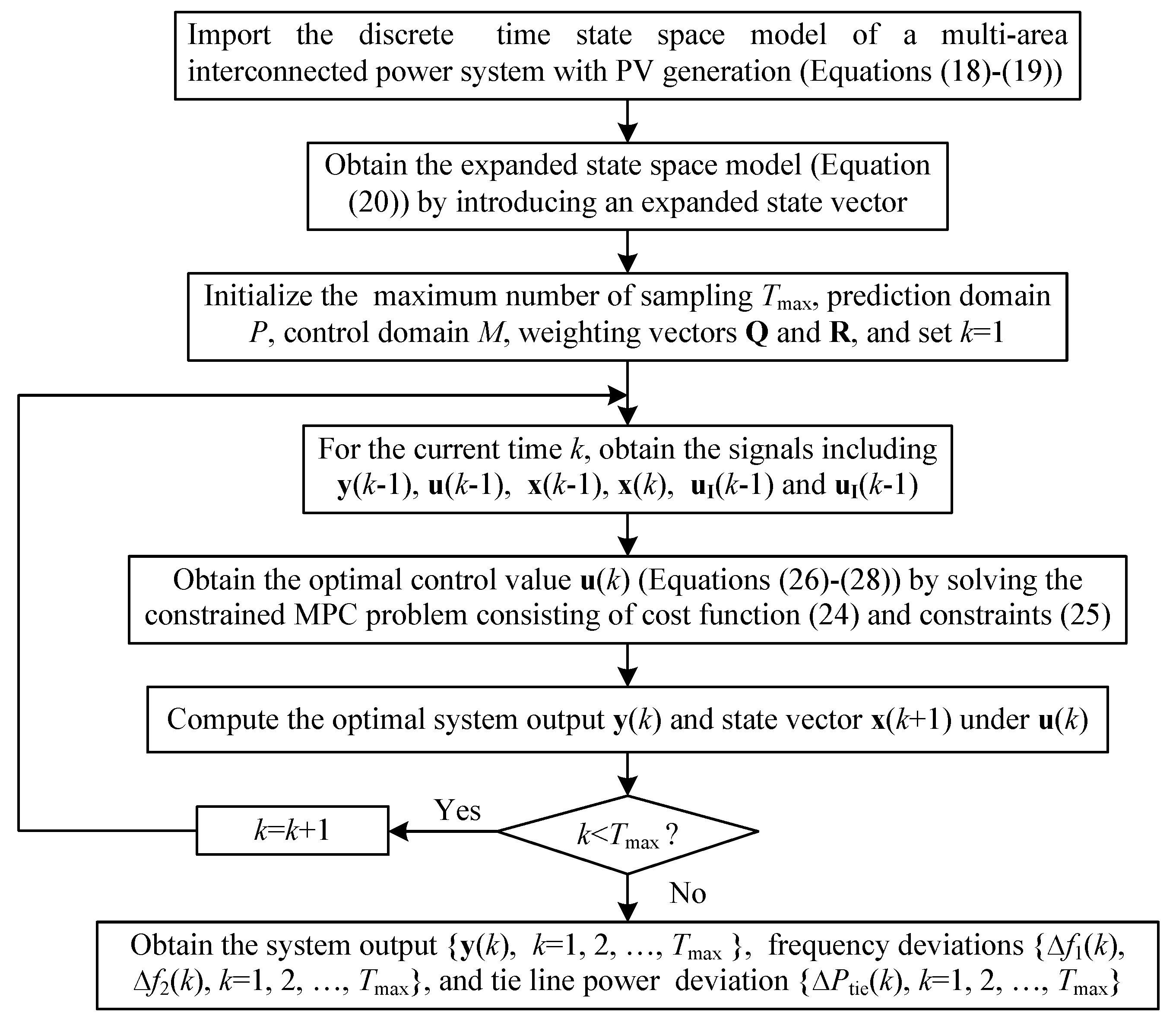
Import the discrete time state space model of a multi-area interconnected power system with PV generation described as Equations (18) and (19).

Step 2:

Obtain the expanded state space model described as Equation (20) by introducing an expanded state vector.

Step 3:

Initialize the parameters of predictive control model including maximum number of sampling T_max, prediction domain P, control domain M, weighting vectors Q and R, and set k=1;

Step 4:

For the current time k, obtain the past values of the output vector y(k − 1) = [ACE₁(k − 1), ACE₂(k − 1)]^T, control vector u(k − 1) = [ΔP_c1(k − 1), ΔP_c2(k − 1)]^T, state vector x(k − 1) = [ΔP₁(k − 1), ΔP_pv(k − 1), ΔP_tie(k − 1), Δf₂(k − 1), ΔP₃(k − 1), ΔP₄(k − 1), ΔP₅(k − 1)]^T, and disturbance vector u_I(k − 1) = [ΔP_L1(k − 1), ΔP_L2(k − 1), ΔP_L3(k − 1)]^T.

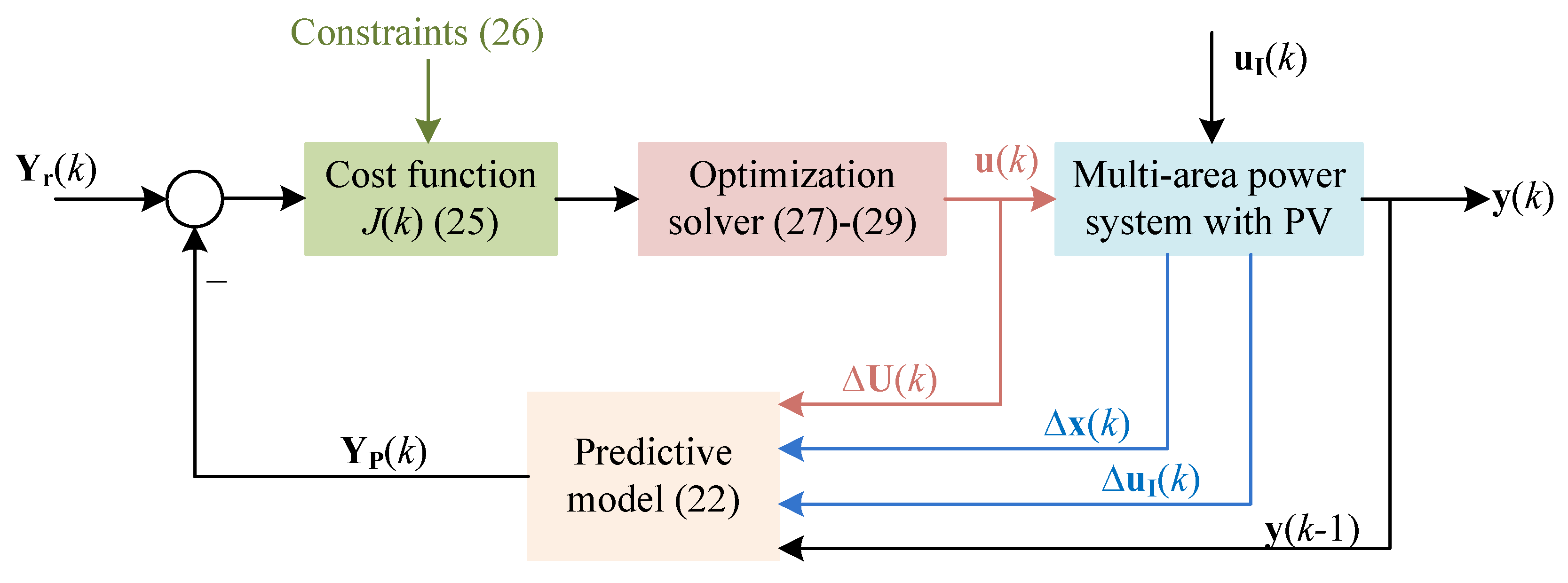
Step 5:

Obtain the predictive vector Y_P(k) by Equation (22) and the rolling optimization model consisting of cost function (25) and constraints (26).

Step 6:

Obtain the optimal control vector u(k) according to Equations (27)–(29) by gradient descent method.

Step 7:

Compute the optimal system output y(k) and state vector x(k) under u(k).

Step 8:

Set k = k + 1, and return step 4 until k = T_max.

Step 9:

Obtain the system output {y(k), k=1, 2, …, T_max}, frequency deviation {Δf₁(k), Δf₂(k), k=1, 2, …, T_max}, and tie line power{ΔP_tie(k), k=1, 2, …, T_max} of a multi-area interconnected power system with PV generation.

4. Simulation Results

In order to demonstrate the effectiveness of the proposed MPC method, this section presents the simulation results on a two-area interconnected power system with PV generation. The system parameters are set as: T_p = 20 s, T_t = 0.3 s, T_r = 10 s, T₁₂ = 0.545 p.u., T_g = 0.08 s, K_P = 120 Hz/p.u. MW, K_g = K_t = 1 Hz/p.u.MW, K_r = 3.3 Hz/p.u MW, B = 0.8 p.u.MW/Hz, R = 0.4 Hz/p.u.MW, K_r1 = 0.33p.u. MW, a₁ = 99.5, a₃ = 0.5, a₂ = −50, K₁ = −18. According to the previous research work [44,45], the maximum value of DB for governor is set as 0.05 p.u., and the GRC value is specified as 10% per minute.

The comparative methods include firefly algorithm (FA)-based PI controller abbreviated as FA-PI [32], genetic algorithm (GA)-based PI controller abbreviated as GA-PI [32], and our recently reported population extremal optimization (PEO)-based PI controller abbreviated as PEO-PI [42,43]. For fair comparison, the lower and upper limits of the optimized PI controllers’ parameters are set as −2 and 2 for FA-PI, GA-PI and PEO-PI, respectively [32]. The parameters setting of MPC and three mentioned evolutionary algorithms based PI methods are shown in

Table 1. The parameters setting of MPC, PEO-PI, GA-PI and FA-PI.

Algorithm	Parameters Setting
FA-PI [32]	Number of fireflies = 50, maximum number of generations = 100, the contrast of the attractiveness =1.0, the attractiveness = 0.1 at r = 0, randomization = 0.1.
GA-PI [32]	Population size = 50, maximum number of generations = 100, the crossover probability pc = 0.75, the mutation probability pm = 0.1.
PEO-PI [43]	Population size = 30,maximum number of generations = 100, shape parameter of MNUM mutation b = 2.
MPC	Prediction horizon P = 15, control horizon M = 10, weight vectors Q = EP×P, R = 0.01EM×M.

.

Table 2. Theconditions of experiments.

Experiment	Condition
Case 1	Step increase in demand of thermal system, i.e., ΔPL1 = 0.1
Case 2	Step increase in demand of thermal system and PV generation, i.e., ΔPL1 = 0.1 and ΔPL2 = 0.1
Case 3	Parameter Tg increases and decreases 40% under ΔPL1 = 0.1 and ΔPL2 = 0.1
Case 4	Parameter Tt increases and decreases 40% under ΔPL1 = 0.1 and ΔPL2 = 0.1
Case 5	Dynamical fluctuations of ΔPL1
Case 6	Dynamical fluctuations of ΔPL2

presents four experimental conditions and all the following simulations is implemented on by MATLAB 2012b software on a 2.50 GHz PC with i7-3537U processor and 4 GB RAM.

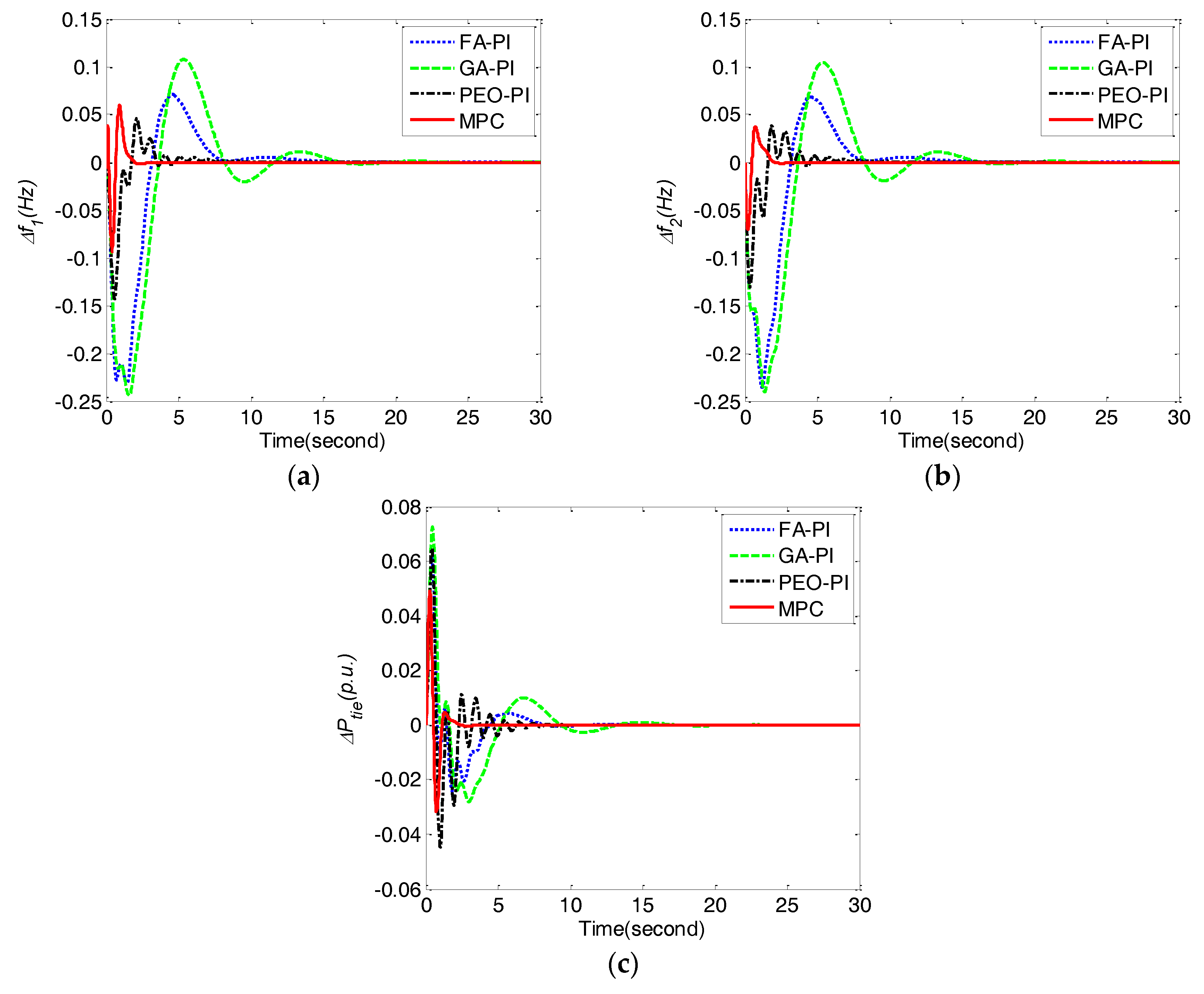
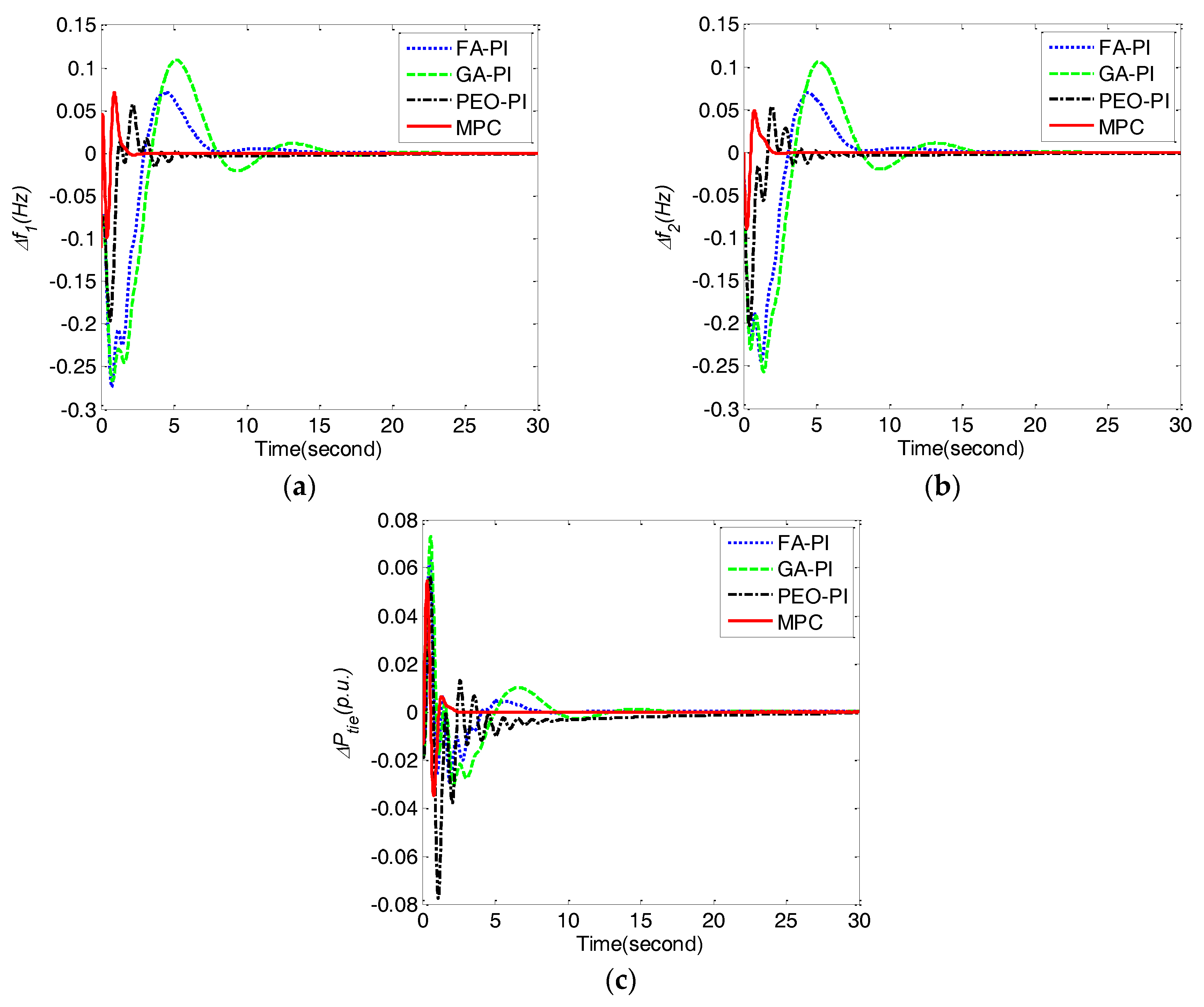
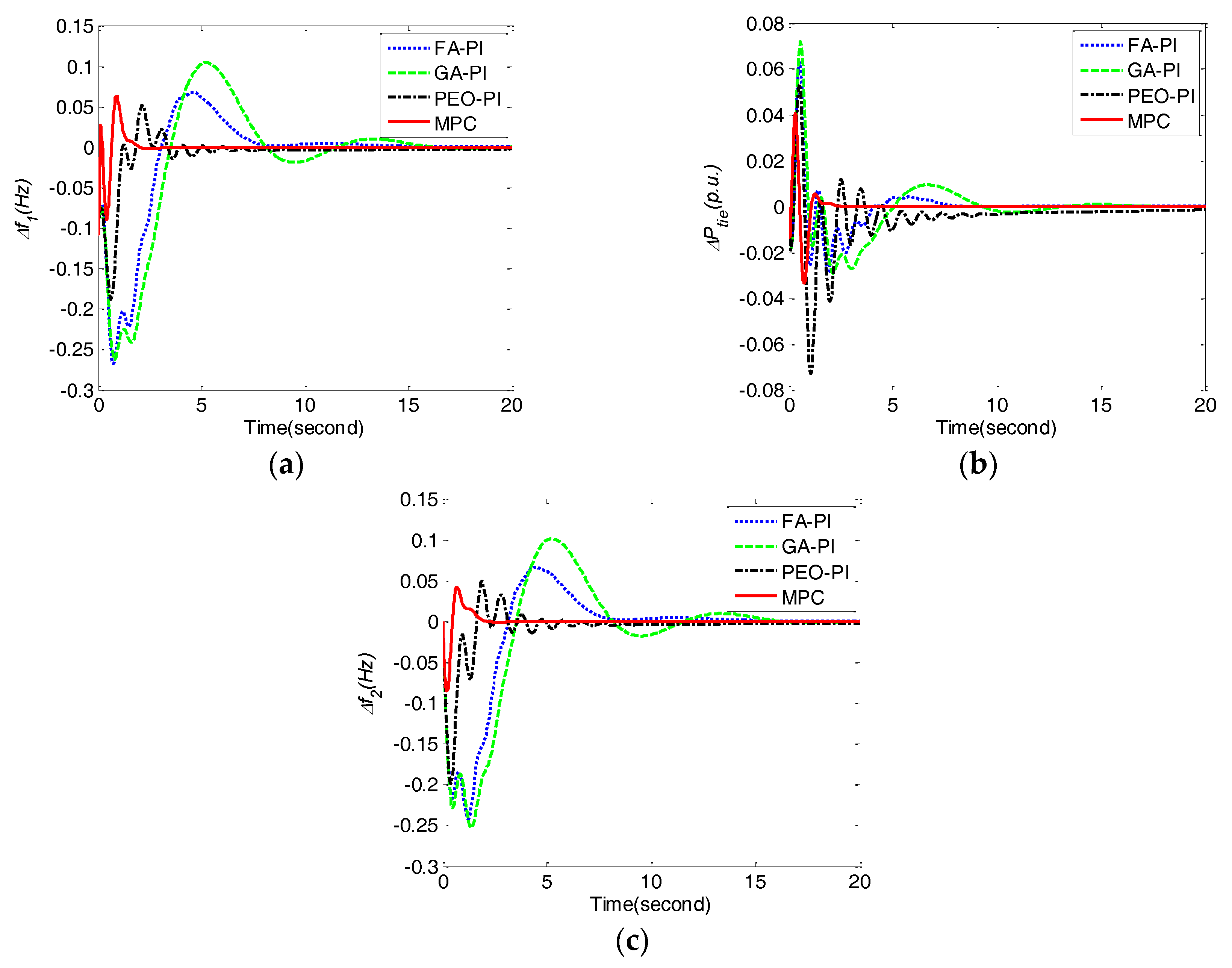
4.1. Case 1: Step Increase in Demand of Thermal System

Table 3. Optimized PI parameters obtained by PEO-PI, GA-PI and FA-PI.

Algorithm	KP1	KI1	KP2	KI2
FA−PI [32]	−0.8811	−0.5765	−0.7626	−0.8307
GA−PI [32]	−0.5663	−0.4024	−0.5127	−0.7256
PEO−PI [43]	−0.8749	−0.1373	−1.999	−1.9487

presents the optimized PI parameters including K_P1, K_I1, K_P2, and K_I2 obtained by PEO-PI, GA-PI and FA-PI for case 1. Frequency deviations Δf₁, Δf₂, and tie line power deviation ΔP_tie obtained by MPC, PEO-PI, GA-PI and FA-PI for case 1 are shown in Figure 4 and the corresponding performance of is compared in

Table 4. Performance comparison of MPC, PEO-PI, GA-PI and FA-PI for case 1.

Algorithm	IAE	ITAE	ISE	ITSE	Mp1	tu1	ts1	Ess1	Mp2	tu2	ts2	Ess2	Mp3	tu3	ts3	Ess3
FA-PI	41.38	117.76	5.29	8.83	0.07	3.12	11.75	1.89 × 10−5	0.07	3.15	11.71	2.22 × 10−5	0.06	3.85	3.85	5.68 × 10−7
GA-PI	59.32	227.11	7.60	18.03	0.11	3.61	15.11	1.30 × 10−4	0.10	3.63	15.11	1.02 × 10−4	0.07	4.83	8.28	5.87 × 10−6
PEO-PI	11.07	19.80	0.63	0.49	0.05	1.73	5.22	1.34 × 10−5	0.04	1.57	5.92	1.18 × 10−5	0.06	1.34	3.67	1.09 × 10−5
MPC	8.83	6.07	0.39	0.20	0.06	0.67	1.68	3.05 × 10−6	0.04	0.47	1.73	1.13 × 10−7	0.05	1.08	1.32	4.63 × 10−8

. The performance indices include the integral of absolute value of the error (IAE), the integral of time multiplied absolute value of the error (ITAE), the integral of square error (ISE), the integral of time multiplied square error (ITSE), the overshoot of Δf₁, Δf₂ and ΔP_tie denoted asM_p1, M_p2 and M_p3,respectively, the rising time of Δf₁, Δf₂ and ΔP_tie denoted as t_r1, t_r2 and t_r3, respectively, settling time of Δf₁, Δf₂ and ΔP_tie denoted as t_s1, t_s2 and t_s3, respectively, the steady-state error of Δf₁, Δf₂ and ΔP_tie denoted as E_ss1, E_ss2 and E_ss3, respectively. More specifically, IAE, ITAE, ISE and ITSE are defined as follows [32]:

$$IAE={\displaystyle {\int }_0^{T_{\max }}\left(\left|\Delta f_1\right|+\left|\Delta f_2\right|+\left|\Delta P_{\mathrm{tie}}\right|\right)}dt,$$

(30)

$$ITAE={\displaystyle {\int }_0^{T_{\max }}t\left(\left|\Delta f_1\right|+\left|\Delta f_2\right|+\left|\Delta P_{\mathrm{tie}}\right|\right)}dt,$$

(31)

$$ISE={\displaystyle {\int }_0^{T_{\max }}\left({\left(\Delta f_1\right)}^2+{\left(\Delta f_2\right)}^2+{\left(\Delta P_{\mathrm{tie}}\right)}^2\right)}dt,$$

(32)

$$ITSE={\displaystyle {\int }_0^{T_{\max }}t\left({\left(\Delta f_1\right)}^2+{\left(\Delta f_2\right)}^2+{\left(\Delta P_{\mathrm{tie}}\right)}^2\right)}dt.$$

(33)

From Table 4, it is clear that MPC performs better than FA-PI, GA-PI and PEO-PI in the terms of all of the performance indices.

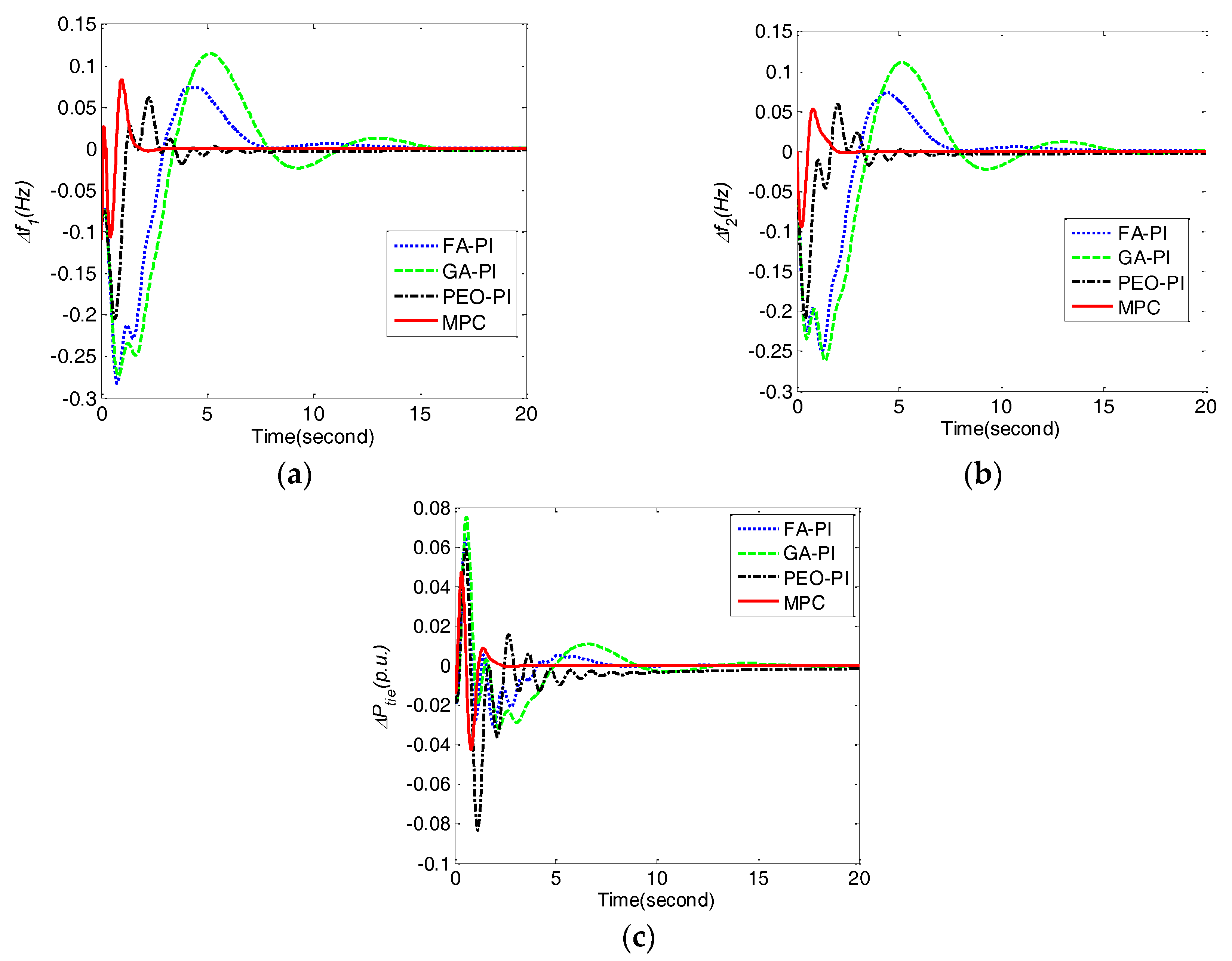
4.2. Case 2: Step Increase in Demand of Thermal System and PVGeneration

For case 2, the frequency deviations Δf₁, Δf₂, and tie line power deviation ΔP_tie obtained by MPC, PEO-PI, GA-PI and FA-PI under ΔP_L1 = 0.1 and ΔP_L2 = 0.1 are shown in Figure 5 and the corresponding performance indices of are compared in

Table 5. Performance comparison of MPC, PEO-PI, GA-PI and FA-PI for case 2.

Algorithm	IAE	ITAE	ISE	ITSE	Mp1	tu1	ts1	Ess1	Mp2	tu2	ts2	Ess2	Mp3	tu3	ts3	Ess3
FA-PI	42.99	114.54	5.77	8.69	0.07	2.94	11.67	1.98 × 10−5	0.07	3.07	11.64	2.17 × 10−5	0.06	3.84	3.84	5.08 × 10−7
GA-PI	60.80	221.79	8.29	17.81	0.11	3.43	14.95	1.07 × 10−4	0.11	3.5	14.97	9.82 × 10−5	0.07	4.63	8.14	7.70 × 10−6
PEO-PI	21.27	86.77	1.66	1.21	0.06	1.17	4.91	7.84 × 10−4	0.05	1.66	5.55	7.89 × 10−4	0.06	1.53	7.19	6.29 × 10−4
MPC	11.25	7.01	0.63	0.27	0.07	0.23	1.75	5.11 × 10−6	0.05	0.49	1.78	1.13 × 10−7	0.05	1.10	1.48	4.63 × 10−8

. Obviously, all of the indices obtained by MPC are the best among the four methods.

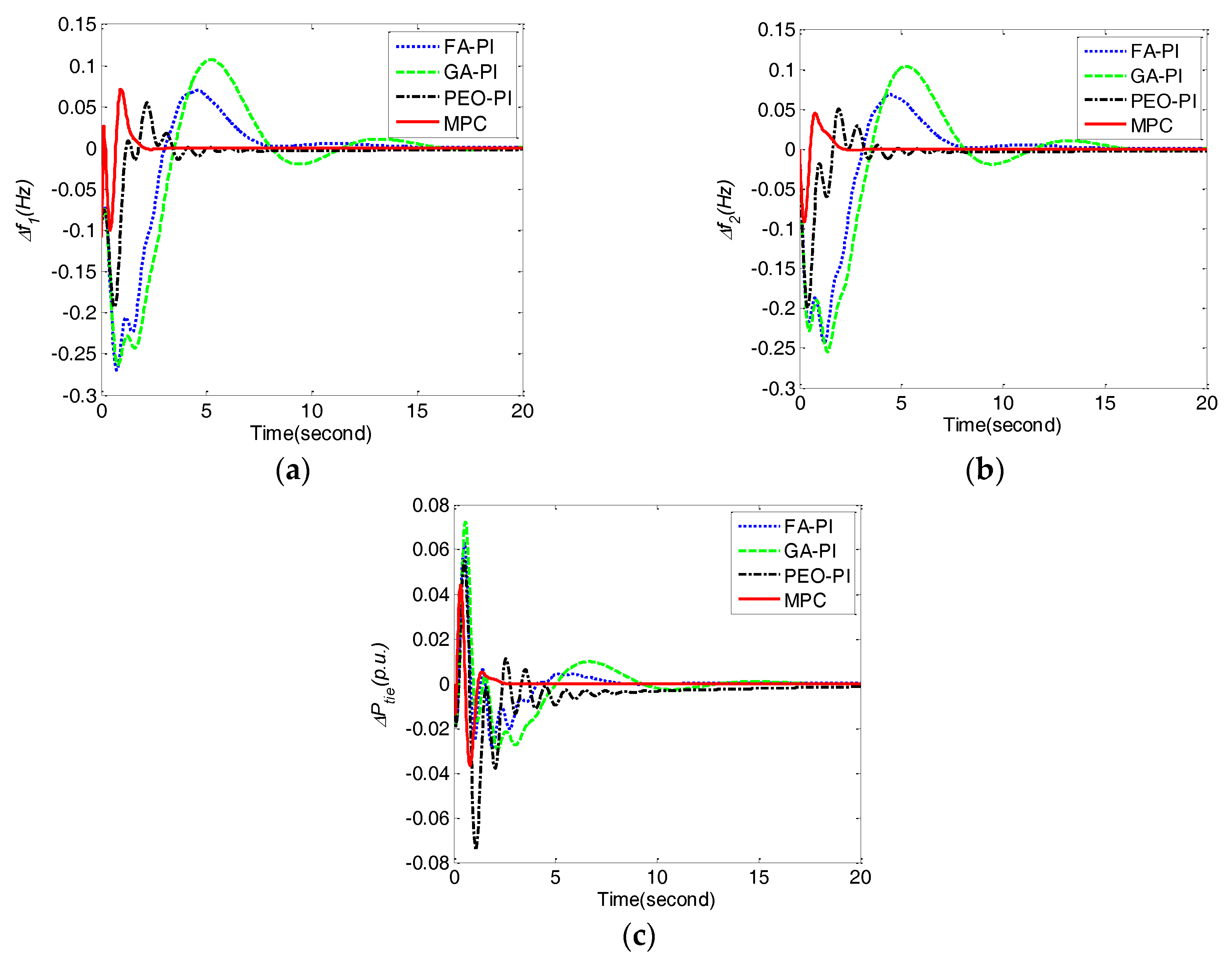
4.3. Case 3: Robustness Test for Perturbed Parameter T_g

In order to demonstrate the robustness of the proposed method against parameters uncertainty, the experiments have been implemented when parameter T_g increases and decreases 40%under ΔP_L1 = 0.1 and ΔP_L2 = 0.1.

Table 6. Performance comparison of MPC, PEO-PI, GA-PI and FA-PI for case 3.

Algorithm	Condition	IAE	ITAE	ISE	ITSE
FA-PI [32]	Tg increases 40%	43.36	113.56	6.01	9.04
GA-PI [32]		62.65	225.38	8.72	18.81
PEO-PI [43]		19.93	62.22	1.66	1.24
MPC		10.97	7.38	0.66	0.33
FA-PI [32]	Tg decreases 40%	42.38	112.71	5.65	8.55
GA-PI [32]		60.54	213.73	8.22	17.48
PEO-PI [43]		19.3	60.93	1.53	1.11
MPC		10.21	6.60	0.58	10.26

presents the performance comparison under two conditions including T_g increasing 40% and decreasing 40%. Clearly, MPC performs the best in terms of IAE, ITAE, ISE and ITSE under all of the conditions. Furthermore, the dynamic responses of the frequency deviations Δf₁, Δf₂, and tie line power deviation ΔP_tie obtained by MPC, PEO-PI, GA-PI and FA-PI under T_g increasing 40% and decreasing 40% are shown in Figure 6 and Figure 7, respectively. MPC obtained less fluctuations, faster responses and better steady-state performance than PEO-PI, GA-PI and FA-PI when parameter T_g mismatches.

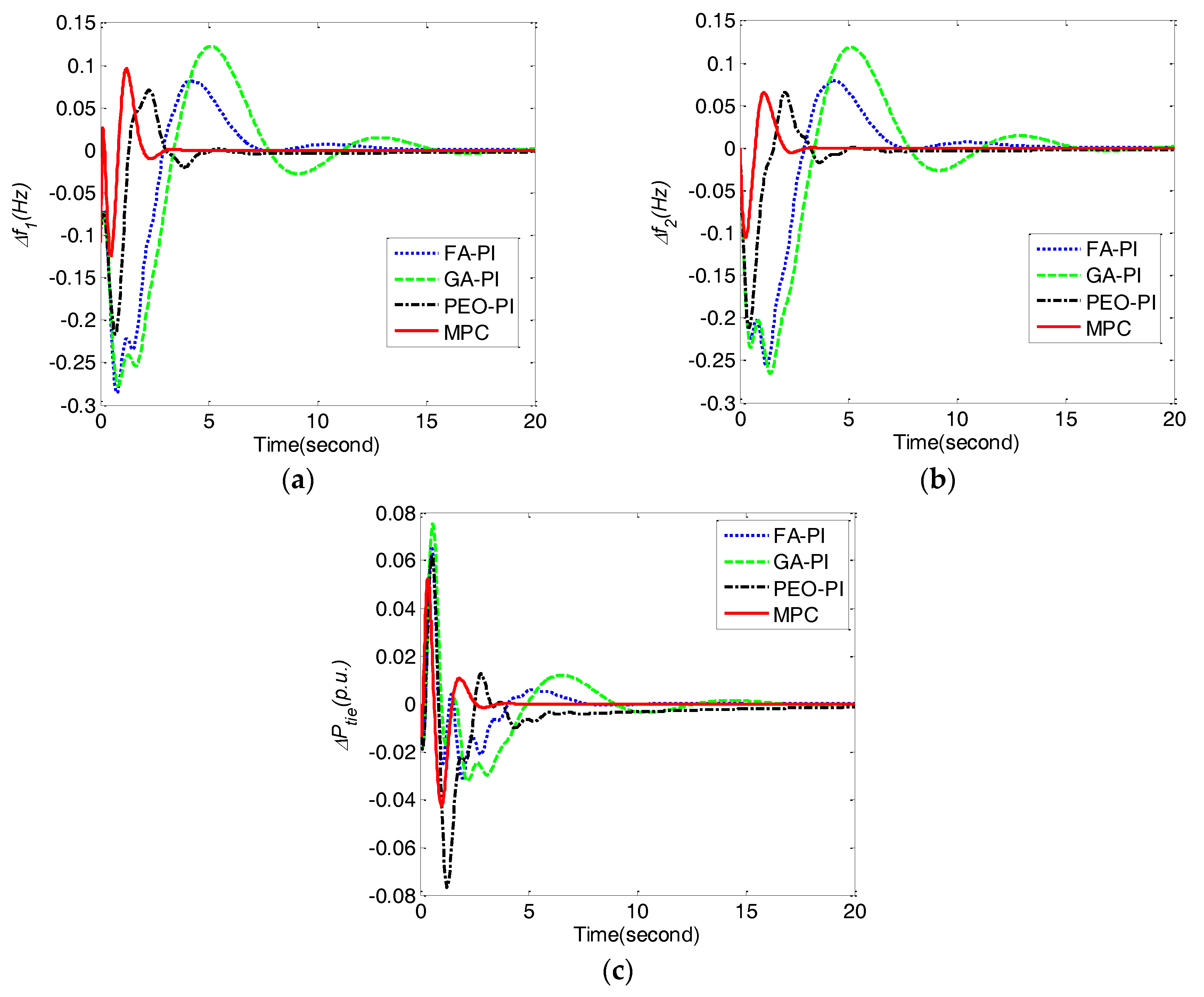
4.4. Case 4: Robustness Test for Perturbed Parameter T_t

Table 7. Performance comparison of MPC, PEO-PI, GA-PI and FA-PI for case 4.

Algorithm	Condition	IAE	ITAE	ISE	ITSE
FA-PI [32]	Tt increases 40%	44.68	115.67	6.35	9.69
GA-PI [32]		64.83	241.76	9.14	20.39
PEO-PI [43]		22.71	66.65	1.98	1.64
MPC		14.83	12.63	1.00	0.68
FA-PI [32]	Tt decreases 40%	42.36	112.38	5.57	8.39
GA-PI [32]		59.21	209.39	8.00	17.02
PEO-PI [43]		19.32	61.32	1.47	1.06
MPC		9.04	5.25	0.48	0.18

presents the performance comparison under two conditions including T_t increasing 40% and decreasing 40% when ΔP_L1 = 0.1 and ΔP_L2 = 0.1. It is obvious that IAE, ITAE, ISE and ITSE obtained by MPC are all better than FA-PI, GA-PI and PEO-PI under all the conditions. The dynamic responses of the frequency deviations Δf₁, Δf₂, and tie line power deviation ΔP_tie obtained by MPC, PEO-PI, GA-PI and FA-PI under T_t increasing 40% and decreasing 40% are shown in Figure 8 and Figure 9, respectively. Cleary, MPC is still prior to PEO-PI, GA-PI and FA-PI in terms of both transient and steady-state performance under the variations of parameter T_t.

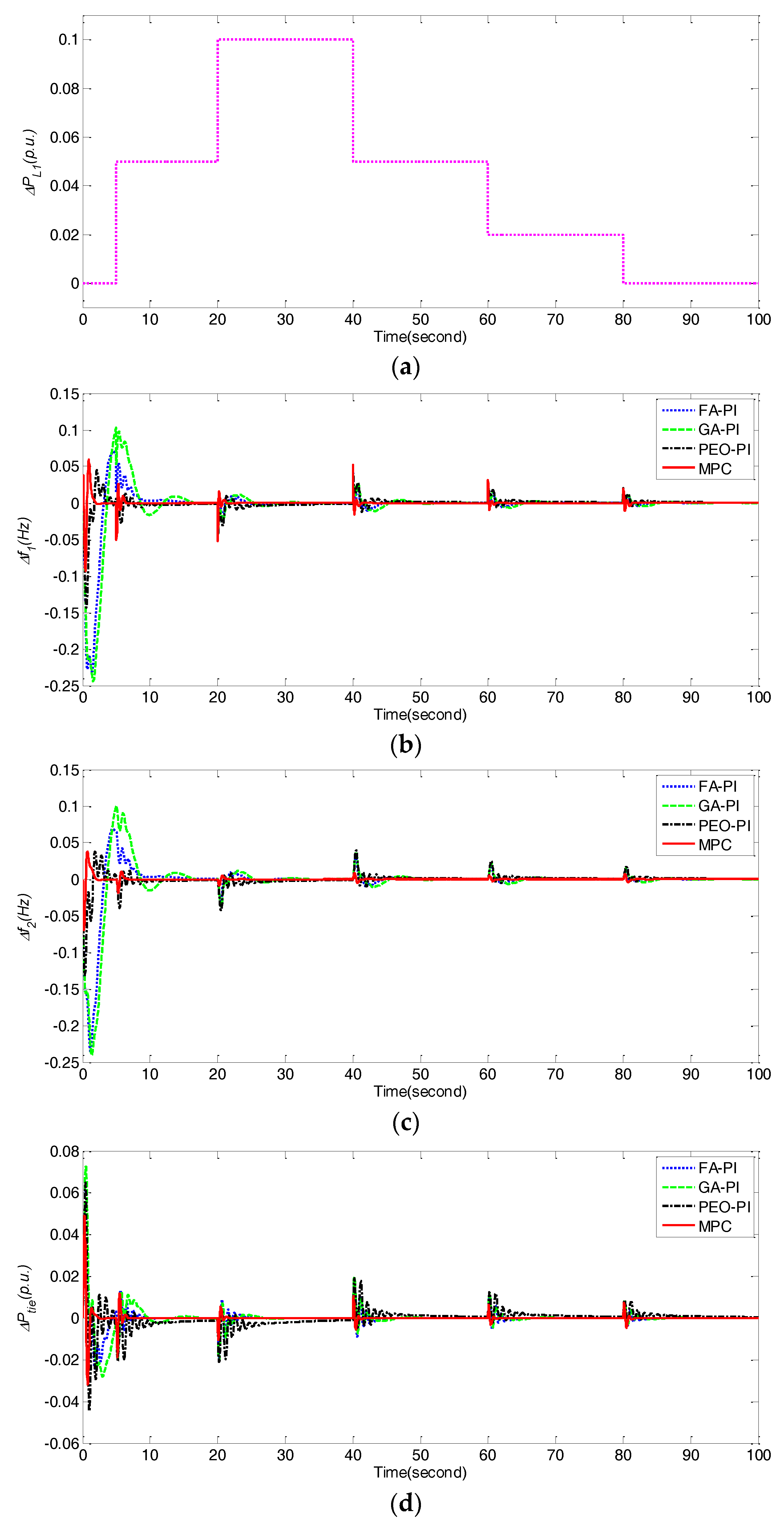
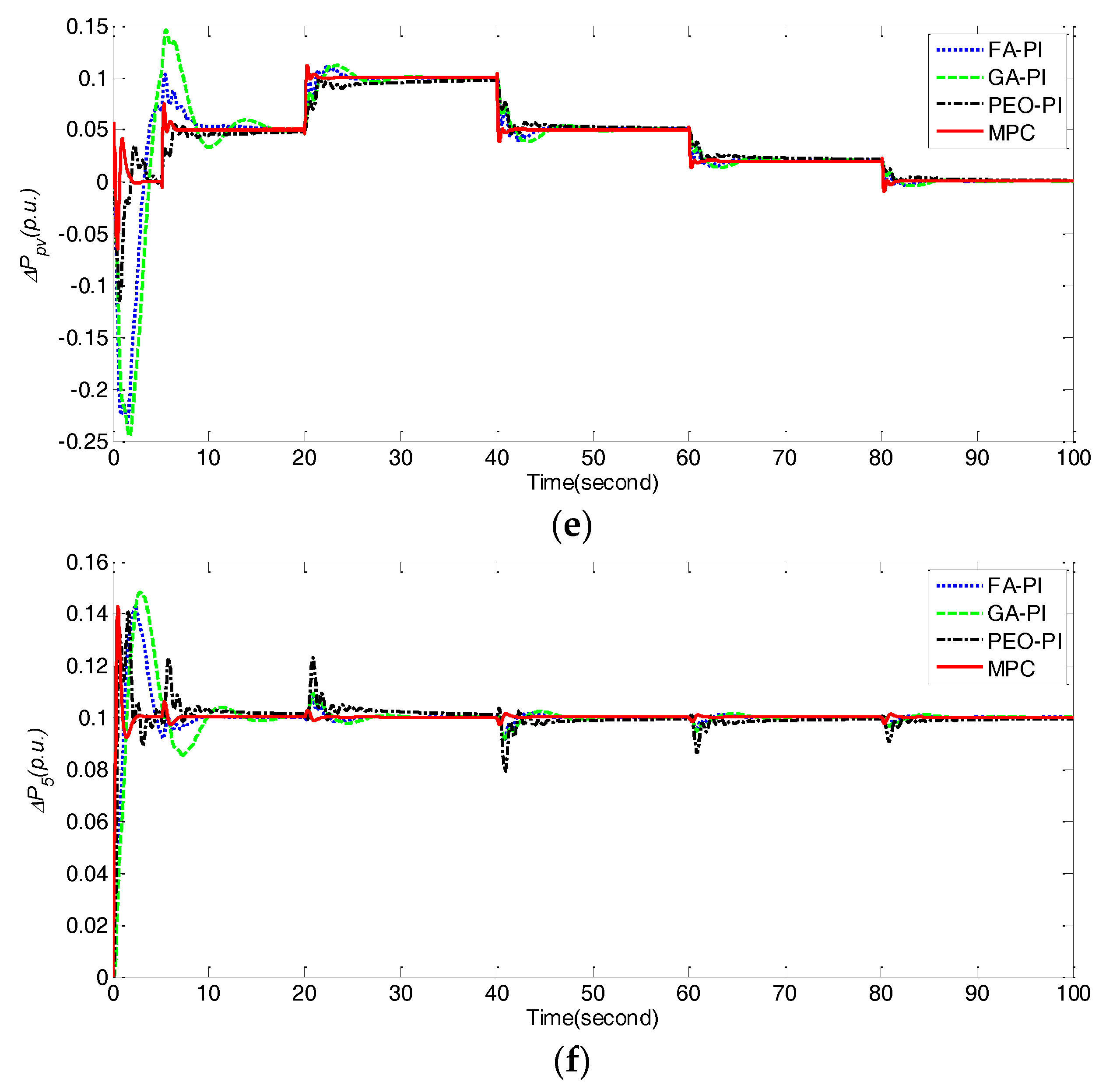
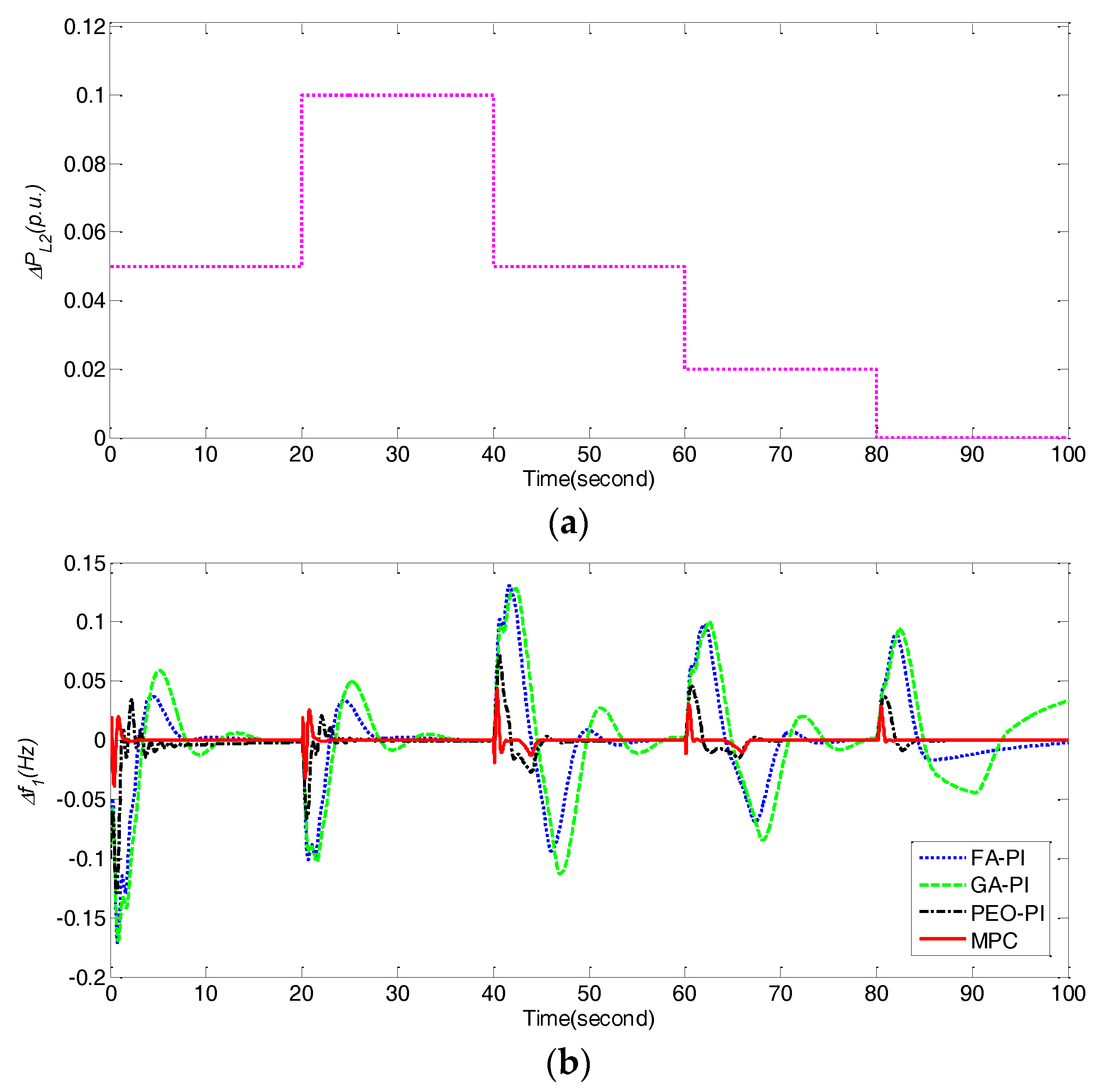
4.5. Robustness Test for Dynamical Load Fluctuations

In this subsection, two experiments have been done to further demonstrate the robustness of the proposed MPC method for the dynamical loads fluctuations of ΔP_L1 and ΔP_L2. More specifically, Figure 10 and Figure 11 show the dynamic responses of frequency deviations Δf₁, Δf₂, and power deviations ΔP_tie, ΔP_pv, ΔP₅ obtained by different control methods under dynamical fluctuations of ΔP_L1 and ΔP_L2, respectively. It is obvious that the proposed MPC performs better than PEO-PI, GA-PI and FA-PI due to its fast transient responses and less deviations of Δf₁, Δf₂, ΔP_tie, ΔP_pv, and ΔP₅ under two conditions. Moreover,

Table 8. Performance comparison of MPC, PEO-PI, GA-PI and FA-PI for dynamical load fluctuations.

Algorithm	Condition	IAE	ITAE	ISE	ITSE
FA-PI [32]	Case 5:Dynamical fluctuationsof ΔPL1	50.18	502.38	5.35	12.58
GA-PI [32]		71.70	829.83	7.57	22.8
PEO-PI [43]		32.60	908.93	0.85	7.12
MPC		12.78	161.44	0.42	2.03
FA-PI [32]	Case 6: Dynamical fluctuationsof ΔPL2	133.27	6034.24	8.62	341.94
GA-PI [32]		196.33	9514.9	12.8	541.8
PEO-PI [43]		39.06	1287.35	1.3	28.93
MPC		14.02	468.56	0.32	6.92

further compares the performance indices such as IAE, ITAE, ISE and ITSE obtained by different control methods under two cases of dynamical load fluctuations. Clearly, MPC is superior to FA-PI, GA-PI and PEO-PI in terms of all indices. In other words, the proposed MPC method in this paper also outperforms these state-of-the-art PI control methods [32,43] for the LFC issue of a multi-area interconnected power system with PV generations even under the dynamical loads fluctuations.

5. Conclusions

In this paper, an adaptive model predictive control (MPC) method is proposed for load frequency control (LFC) issue of a multi-area interconnected power system with PV generation. The key operations of this proposed method include formulating the LFC issue as a discrete-time state space model, obtaining the dynamic predictive model by introducing an expanded state vector, and rolling optimization of control output signal by gradient descent method based on a cost function minimizing the weighted sum of square predicted errors and square future control values. The simulation results on a typical two-area power system consisting of photovoltaic and thermal generator have shown that the proposed MPC method is superior to evolutionary algorithms-based PI control methods such as FA-PI [32], GA-PI [32], and PEO-PI [42,43] in terms of dynamic and steady-state performance in cases of normal condition, load disturbance and parameters uncertainty. To the best of the authors’ knowledge, this work can be considered as the first contribution of MPC to the optimal LFC issue of a multi-area interconnected power system with PV generation. However, from the theoretical perspective, the optimal design issue of the weighting vectors, prediction horizon and control horizon in the proposed MPC method is still challenging. From the perspective of engineering practice, the proposed method will be further studied in depth by tuning the weighting vectors, prediction horizon and control horizon based on evolutionary algorithms, such as multi-objective optimization algorithms [46,47,48]. On the other hand, the extension of MPC to more complex power systems by taking into account the robust control performance indices [45] and real-time predictive power of renewable energy systems [49] is another significant subject of future investigation.

References

1. Pandey, S.K.; Mohanty, S.R.; Kishor, N. A literature survey on load-frequency control for conventional and distribution generation power systems. Renew. Sustain. Energy Rev. 2013, 25, 318–334. [Google Scholar] [CrossRef]
2. Wu, Y.; Wei, Z.; Weng, J.; Li, X.; Deng, R.H. Resonance attacks on load frequency control of smart grids. IEEE Trans. Smart Grid 2017. [Google Scholar] [CrossRef]
3. Tan, W. Unified tuning of PID load frequency controller for power systems via IMC. IEEE Trans. Power Syst. 2010, 25, 341–350. [Google Scholar] [CrossRef]
4. Saxena, S.; Hote, Y.V. Decentralized PID load frequency control for perturbed multi-area power systems. Int. J. Electr. Power Energy Syst. 2016, 81, 405–415. [Google Scholar] [CrossRef]
5. Golpira, H.; Bevrani, H. Application of GA optimization for automatic generation control design in an interconnected power system. Energy Convers. Manag. 2011, 52, 2247–2255. [Google Scholar] [CrossRef]
6. Daneshfar, F.; Bevrani, H. Multiobjective design of load frequency control using genetic algorithms. Int. J. Electr. Power Energy Syst. 2012, 42, 257–263. [Google Scholar] [CrossRef]
7. Naidu, K.; Mokhlis, H.; Bakar, A.H.A. Multiobjective optimization using weighted sum artificial bee colony algorithm for load frequency control. Int. J. Electr. Power Energy Syst. 2014, 55, 657–667. [Google Scholar] [CrossRef]
8. Panda, S.; Yegireddy, N.K. Automatic generation control of multi-area power system using multi-objective non-dominated sorting genetic algorithm-II. Int. J. Electr. Power Energy Syst. 2013, 53, 54–63. [Google Scholar] [CrossRef]
9. Chuang, N. Robust H∞ load-frequency control in interconnected power systems. IET Control Theory Appl. 2016, 10, 67–75. [Google Scholar] [CrossRef]
10. Ersdal, A.M.; Lars, I.; Kjetil, U. Model predictive load-frequency control. IEEE Trans. Power Syst. 2016, 31, 777–785. [Google Scholar] [CrossRef]
11. Ojaghi, P.; Rahmani, M. LMI-based robust predictive load frequency control for power systems with communication delays. IEEE Trans. Power Syst. 2017, 32, 4091–4100. [Google Scholar] [CrossRef]
12. Liu, X.; Kong, X.; Lee, K.Y. Distributed model predictive control for load frequency control with dynamic fuzzy valve position modeling for hydro–thermal power system. IET Control Theory Appl. 2016, 10, 1653–1664. [Google Scholar] [CrossRef]
13. Ersdal, A.M.; Imsland, L.; Uhlen, K.; Fabozzi, D.; Thornhill, N.F. Model predictive load-frequency control taking into account imbalance uncertainty. Control Eng. Pract. 2016, 53, 139–150. [Google Scholar] [CrossRef]
14. Ma, M.; Zhang, C.; Liu, X.; Chen, H. Distributed model predictive load frequency control of multi-area power system after deregulation. IEEE Trans. Ind. Electron. 2017, 64, 5129–5139. [Google Scholar] [CrossRef]
15. Mi, Y.; Fu, Y.; Wang, C.; Wang, P. Decentralized sliding mode load frequency control for multi-area power systems. IEEE Trans. Power Syst. 2013, 28, 4301–4309. [Google Scholar] [CrossRef]
16. Prasad, S.; Purwar, S.; Kishor, N. Non-linear sliding mode load frequency control in multi-area power system. Control Eng. Pract. 2017, 61, 81–92. [Google Scholar] [CrossRef]
17. Sabahiand, K.; Teshnehlab, M. Recurrent fuzzy neural network by using feedback error learning approaches for LFC in interconnected power system. Energy Convers. Manag. 2009, 50, 938–946. [Google Scholar]
18. Saxena, S.; Hote, Y.V. Stabilization of perturbed system via IMC: An application to load frequency control. Control Eng. Pract. 2017, 64, 61–73. [Google Scholar] [CrossRef]
19. Chen, H.Y.; Ye, R.; Wang, X.D.; Lu, R.G. Cooperative control of power system load and frequency by using differential games. IEEE Trans. Control Syst. Technol. 2015, 23, 882–897. [Google Scholar] [CrossRef]
20. Panda, S.; Mohanty, B.; Hota, P.K. Hybrid BFOA-PSO algorithm for automatic generation control of linear and nonlinear interconnected power systems. Appl.Soft Comput. 2013, 13, 4718–4730. [Google Scholar] [CrossRef]
21. Sahu, R.K.; Panda, S.; Rout, U.K. DE optimized parallel 2-DOF PID controller for load frequency control of power system with governor dead-band nonlinearity. Int. J. Electr. Power Energy Syst. 2013, 49, 19–33. [Google Scholar] [CrossRef]
22. Mohanty, B.; Panda, S.; Hota, P.K. Controller parameters tuning of differential evolution algorithm and its application to load frequency control of multi-source power system. Int. J. Electr. Power Energy Syst. 2014, 54, 77–85. [Google Scholar] [CrossRef]
23. Rakhshani, E.; Luna, A.; Rouzbehi, K.; Rodriguez, P. Application of imperialist competitive algorithm to design an optimal controller for LFC problem. In Proceedings of the 38th Annual Conference on IEEE Industrial Electronics Society, Montreal, QC, Canada, 25–28 October 2012; pp. 1223–1227. [Google Scholar]
24. Padhan, S.; Sahu, R.K.; Panda, S. Application of firefly algorithm for load frequency control of multi-area interconnected power system. Electr. Power Compon. Syst. 2014, 42, 1419–1430. [Google Scholar] [CrossRef]
25. Fini, M.H.; Yousefi, G.R.; Alhelou, H.H. Comparative study on the performance of many-objective and single-objective optimization algorithms in tuning load frequency controllers of multi-area power systems. IET Gener. Transm. Distrib. 2016, 10, 2915–2923. [Google Scholar] [CrossRef]
26. Mohamed, T.H.; Morel, J.; Bevrani, H.; Hiyama, T. Model predictive based load frequency control design concerning wind turbines. Int. J. Electr. Power Energy Syst. 2012, 43, 859–867. [Google Scholar] [CrossRef]
27. Bevrani, H.; Daneshmand, P.R. Fuzzy logic-based load-frequency control concerning high penetration of wind turbines. IEEE Syst. J. 2012, 6, 173–180. [Google Scholar] [CrossRef]
28. Qian, D.; Tong, S.; Liu, H.; Liu, X. Load frequency control by neural-network-based integral sliding mode for nonlinear power systems with wind turbines. Neurocomputing 2016, 173, 875–885. [Google Scholar] [CrossRef]
29. Liu, X.; Zhang, Y.; Lee, K.Y. Coordinated distributed MPC for load frequency control of power system with wind farms. IEEE Trans. Ind. Electron. 2017, 64, 5140–5150. [Google Scholar] [CrossRef]
30. Ma, M.; Liu, X.; Zhang, C. LFC for multi-area interconnected power system concerning wind turbines based on DMPC. IET Gener. Transm. Distrib. 2017, 11, 2689–2696. [Google Scholar] [CrossRef]
31. Kumar, L.S.; Kumar, G.N.; Madichetty, S. Pattern search algorithm based automatic online parameter estimation for AGC with effects of wind power. Int. J. Electr. Power Energy Syst. 2017, 84, 135–142. [Google Scholar] [CrossRef]
32. Abd-Elazim, S.M.; Ali, E.S. Load frequency controller design of a two-area system composing of PV grid and thermal generator via firefly algorithm. Neural Comput. Appl. 2016. [Google Scholar] [CrossRef]
33. Camacho, E.F.; Alba, C.B. Model Predictive Control; Springer Science & Business Media: Berlin, Germany, 2013. [Google Scholar]
34. Mayne, D.Q. Model predictive control: Recent developments and future promise. Automatica 2014, 50, 2967–2986. [Google Scholar] [CrossRef]
35. Kouro, S.; Cortés, P.; Vargas, R.; Ammann, U.; Rodríguez, J. Model predictive control—A simple and powerful method to control power converters. IEEE Trans. Ind. Electron. 2009, 56, 1826–1838. [Google Scholar] [CrossRef]
36. Rodriguez, J.; Kazmierkowski, M.P.; Espinoza, J.R.; Zanchetta, P.; Abu-Rub, H.; Young, H.A.; Rojas, C.A. State of the art of finite control set model predictive control in power electronics. IEEE Trans. Ind. Inf. 2013, 9, 1003–1016. [Google Scholar] [CrossRef]
37. Vazquez, S.; Leon, J.I.; Franquelo, L.G.; Rodriguez, J.; Young, H.A.; Marquez, A.; Zanchetta, P. Model predictive control: A review of its applications in power electronics. IEEE Ind. Electron. Mag. 2014, 8, 16–31. [Google Scholar] [CrossRef] [Green Version]
38. Geyer, T.; Quevedo, D.E. Performance of multistep finite control set model predictive control for power electronics. IEEE Trans. Power Electron. 2015, 30, 1633–1644. [Google Scholar] [CrossRef]
39. Vazquez, S.; Rodriguez, J.; Rivera, M.; Franquelo, L.G.; Norambuena, M. Model predictive control for power converters and drives: Advances and trends. IEEE Trans. Ind. Electron. 2017, 64, 935–947. [Google Scholar] [CrossRef]
40. Nguyen, T.T.; Yoo, H.J.; Kim, H.M. Analyzing the impacts of system parameters on MPC-based frequency control for a stand-alone microgrid. Energies 2017, 10, 417. [Google Scholar] [CrossRef]
41. Kerdphol, T.; Rahman, F.; Mitani, Y.; Hongesombut, K.; Kufeoglu, S. Virtual inertia control-based model predictive control for microgrid frequency stabilization considering high renewable energy integration. Sustainability 2017, 9, 773. [Google Scholar] [CrossRef]
42. Lu, Y.Z.; Chen, Y.W.; Chen, M.R.; Chen, P.; Zeng, G.Q. Extremal Optimization: Fundamentals, Algorithms, and Applications; CRC Press & Chemical Industry Press: Boca Raton, FL, USA, 2016. [Google Scholar]
43. Zeng, G.Q.; Chen, J.; Chen, M.R.; Dai, Y.X.; Li, L.M.; Lu, K.D.; Zheng, C.W. Design of multivariable PID controllers using real-coded population-based extremal optimization. Neurocomputing 2015, 151, 1343–1353. [Google Scholar] [CrossRef]
44. Mohamed, T.H.; Bevrani, H.; Hassan, A.A.; Hiyama, T. Decentralized model predictive based load frequency control in an interconnected power system. Energy Convers. Manag. 2011, 52, 1208–1214. [Google Scholar] [CrossRef]
45. Bevrani, H. Robust Power System Frequency Control, 2nd ed.; Springer: New York, NY, USA, 2014. [Google Scholar]
46. Zeng, G.Q.; Chen, J.; Dai, Y.X.; Li, L.M.; Zheng, C.W.; Chen, M.R. Design of fractional order PID controller for automatic regulator voltage system based on multi-objective extremal optimization. Neurocomputing 2015, 160, 173–184. [Google Scholar] [CrossRef]
47. Zeng, G.Q.; Chen, J.; Li, L.M.; Chen, M.R.; Wu, L.; Dai, Y.X.; Zheng, C.W. An improved multi-objective population-based extremal optimization algorithm with polynomial mutation. Inf. Sci. 2016, 330, 49–73. [Google Scholar] [CrossRef]
48. Wang, H.; Zeng, G.Q.; Dai, Y.X.; Bi, D.Q.; Sun, J.L.; Xie, X. Q. Design of fractional order frequency PID controller for an islanded microgrid: A multi-objective extremal optimization method. Energies 2017, 10, 1502. [Google Scholar] [CrossRef]
49. Quan, D.M.; Ogliari, E.; Grimaccia, F.; Leva, S.; Mussetta, M. Hybrid model for hourly forecast of photovoltaic and wind power. In Proceedings of the IEEE International Conference on Fuzzy Systems, Hyderabad, India, 7–10 July 2013; pp. 1–6. [Google Scholar]
Figure 1. The block diagram of a two-area interconnected power system composed of photovoltaic and thermal generator.
Energies 10 01840 g001
Figure 2. The structure of MPC method for the optimal LFC issue of a multi-area interconnected power system with PV generation.
Energies 10 01840 g002
Figure 3. The flowchart of MPC for LFC of a multi-area interconnected power system with PV generation.
Energies 10 01840 g003
Figure 4. Comparison of frequency deviations Δf1, Δf2, and tie line power deviation ΔPtie obtained by different control methods for case 1. (a) frequency deviation Δf1;(b) frequency deviation Δf2; (c) tie line power deviation ΔPtie.
Energies 10 01840 g004
Figure 5. Comparison of frequency deviations Δf1, Δf2, and tie line power deviation ΔPtie obtained by different control methods for case 2. (a) frequency deviation Δf1; (b) frequency deviation Δf2; (c) tie line power deviation ΔPtie.
Energies 10 01840 g005
Figure 6. Comparison of frequency deviations Δf1, Δf2, and tie line power deviation ΔPtie obtained by different control methods under Tg increasing 40% for case 3. (a) frequency deviation Δf1; (b) frequency deviation Δf2; (c) tie line power deviation ΔPtie.
Energies 10 01840 g006
Figure 7. Comparison of frequency deviations Δf1, Δf2 and tie line power deviation ΔPtie obtained by different control methods under Tg decreasing 40%for case 3. (a) frequency deviation Δf1;(b) frequency deviation Δf2; (c) tie line power deviation ΔPtie.
Energies 10 01840 g007
Figure 8. Comparison of frequency deviations Δf1, Δf2 and tie line power deviation ΔPtie obtained by different control methods under Tt increasing 40% for case 4. (a) frequency deviation Δf1;(b) frequency deviation Δf2; (c) tie line power deviation ΔPtie.
Energies 10 01840 g008
Figure 9. Comparison of frequency deviations Δf1, Δf2 and tie line power deviation ΔPtie obtained by different control methods under Tt decreasing 40% for case 4. (a) frequency deviation Δf1;(b) frequency deviation Δf2; (c) tie line power deviation ΔPtie.
Energies 10 01840 g009
Figure 10. Comparison of frequency deviations Δf1, Δf2, and power deviations ΔPtie, ΔPpv, ΔP5 obtained by different control methods under dynamical fluctuations of ΔPL1 for case 5. (a) ΔPL1; (b) Δf1; (c) Δf2; (d) ΔPtie; (e) ΔPpv; (f) ΔP5.
Energies 10 01840 g010aEnergies 10 01840 g010b
Figure 11. Comparison of frequency deviations Δf1, Δf2, and power deviations ΔPtie, ΔPpv, ΔP5 obtained by different control methods under dynamical fluctuations of ΔPL2 for case 6. (a) ΔPL2; (b) Δf1; (c) Δf2; (d) ΔPtie; (e) ΔPpv; (f) ΔP5.
Energies 10 01840 g011aEnergies 10 01840 g011b