Re-Creating Waves in Large Currents for Tidal Energy Applications

Abstract

Unsteady wave loading on tidal turbines impacts significantly the design, and expected life-time, of turbine blades and other key components. Model-scale testing of tidal turbines in the wave-current environment can provide vital understanding by emulating real-world load cases; however, to reduce uncertainty, it is important to isolate laboratory-specific artefacts from real-world behaviour. In this paper, a variety of realistic combined current-wave scenarios is re-created at the FloWave basin, where the main objective is to understand the characteristics of testing in a combined wave-current environment and assess whether wave effects on the flow field can be predicted. Here, we show that a combination of linear wave-current theory and frequency-domain reflection analysis can be used to effectively predict wave-induced particle velocities and identify velocity components that are experimental artefacts. Load-specific mechanisms present in real-world conditions can therefore be isolated, and equivalent full-scale load cases can be estimated with greater confidence. At higher flow speeds, a divergence from the theory presented is observed due to turbulence-induced non-stationarity. The methodology and results presented increase learning about the wave-current testing environment and provide analysis tools able to improve test outputs and conclusions from scale model testing.

1. Introduction

Extracting power from tidal streams is an attractive proposition given the high energy densities available and the predictable and reliable nature of the tidal resource. Recent studies estimate that in the U.K. alone, the technically extractable resource is approximately 29 TWh/year [1], with the value for Europe as a whole being around double this [2]. Tidal power therefore has the potential to be a major contributor to the U.K., European and global energy mix. To extract the available resource, Tidal Stream Turbine (TST) devices have been developed, with the first arrays currently being installed and commissioned [3].

For farms of devices to be viable, TSTs will need to be able to survive very large steady and unsteady hydrodynamic loads over their lifetime. These unsteady loads, depicted in Figure 1, are largely caused by turbulence, waves and shear flow [4] and will induce fatigue in turbine blades and other components. The success of tidal energy devices relies on the prediction of these loads. Wave loads are one of the dominant contributors to fatigue and hence are a key factor in determining turbine blade lifetime [5]. The presence of waves also has implications for control strategies and turbine performance, as discussed in Luznik et al. [6], Fulton et al. [7], Tatum et al. [8].

The extent to which waves will affect a tidal turbine will depend on the device type and the deployment site. The nature of the wave climate itself will clearly have a large influence, as will the available channel depth and rotor position within it. The relative importance of waves for a given application therefore varies; however, in most circumstances, it will play a very significant role in device design and eventual performance. The combined wave-current environment is therefore highly important to characterise, understand and test in.

The presented research is part of the FloWTurb project (Engineering and Physical Sciences Research Council (EPSRC) EP/N021487/1) [9], which aims to “advance the knowledge of how complex wave and tidal current induced turbulence interactions will affect tidal turbine life cycle and performance” [10]. As part of FloWTurb, physical model testing is carried out at the FloWave Ocean Energy Research Facility [11], Edinburgh, U.K., where fully instrumented scaled turbines will be subjected to combined wave-current fields. The first stage of this work is focussed on the process of re-creating observed site conditions and understanding the wave-current testing environment.

The advantage of tank testing to understand more about TSTs, other than cost, is that the environment is very controlled and repeatable. Tank testing aims to understand more about real-world behaviour; however, it is important to identify effects that are tank specific so that they can be considered or removed from equivalent full-scale conclusions. One of the most pertinent of these tank effects is the presence of wave reflection [12], which can cause significant deviation from the specified and desired conditions. Isolation of particle-velocities resulting from incident and reflected waves enables corrections to be applied to measured loads prior to inferring full-scale equivalents. This paper therefore explores the re-creation of combined wave-current conditions at scale for tank testing physical models of TSTs, with the focus on isolating and predicting the effect of wave reflections on the flow field. Baseline flow and turbulence are not focussed on, as this is well described in Sutherland et al. [13]. Namely, this paper details:

• If linear wave-current theory combined with reflection analysis can be used to predict wave-induced water particle velocities (and hence, reduce uncertainty in estimating full-scale wave-induced turbine loads) for waves in fast large currents typical of tidal energy sites
• Experimental results of the decay of wave-induced particle velocities with depth and comparison to the adapted linear wave theory
• Effect of current on the wave fields produced for tank testing
• Issues with re-creating combined wave-current conditions in test tanks

To achieve this, tests were carried out at the FloWave Ocean Energy Research Facility: a combined wave-current test basin located in Edinburgh, U.K. A regular wave case and a selection of observed irregular sea states are (re-)created in following current conditions relating to 1.2, 1.8 and 2.4 m/s full scale. The quality of the generated wave conditions are assessed (stationarity, repeatability, reflections), before theoretical wave-induced particle velocities are compared to measured velocity spectra using an Acoustic Doppler Velocimeter (ADV). If the theory presented can be used to predict the wave-induced velocity spectra in tank experiments, then it should be applicable to site conditions and as inputs to numerical models when it is desired to assess the impact of different wave cases. Importantly, the tools and methodology presented help isolate tank effects from those present in the real world.

The methodology is described in Section 2, which details the calculation of the expected wave-induced particle velocities in a combined wave-current test environment with the presence of wave reflection. The experimental setup and condition definition are presented in Section 3, with results and discussion shown in Section 4. The implications of the results are briefly discussed in Section 5 before conclusions are summarised in Section 6.

2. Theory and Methodology

This section focusses on the prediction of wave effects on current, as the other aspects of the paper either do not require supporting mathematics or are comments based on the observation of the results. It is desired to see if it is possible to predict wave-induced particle velocities. To do this, it is required to first have a good understanding of the waves, which in this environment requires knowledge of how waves and currents interact. In FloWave, or any test tank, wave reflections exist and as such must be quantified and incorporated into the expected particle velocity estimations to allow for valid comparison. This ability also enables attribution of velocities resulting from wave reflection, thus helping isolate tank-effects from ‘real-world-like’ conditions. In Section 2.1, the theory relating to the computation of linear wave-current interaction is described. The calculation of the magnitude of wave reflection in current, and the subsequent effect on water particle velocities in wave-current conditions are detailed in Section 2.2.

2.1. Wave-Current Theory

When waves and currents interact, both current flow and wave fields are modified. The form of the waves can be significantly altered including wave heights, wavelengths and group velocities, which incur a corresponding change in wave steepness and power. Wave-induced particle velocities are introduced into the flow-field, with their magnitude a function of the current-modified wave parameters and the vertical position in the water column, z.

2.1.1. Wave Modification by Current

When waves interact with a current, the wavelengths are modified and are no longer related to frequency through the standard dispersion relation, shown in Equation (1). Jonsson [14] proposed a modified relationship, Equation (2), which is commonly used. Despite temporal and spatial (including shear) variability, flow is approximated as steady, uniform and irrotational throughout all theoretical formulations. In the following equations, subscripts 0 and 1 refer to regions without and with current, respectively, and r corresponds to a reference frame moving at the same velocity as the mean current field.

$$\omega =\sqrt{\mathit{gk}\tanh \mathit{kh}}$$

(1)

$$\omega -k_{1}U=\sqrt{g{k}_1\tanh k_{1}h}$$

(2)

where $\omega$ is angular frequency, which is unchanged in current (rad s${}^{-1}$), k is the wavenumber (m${}^{-1}$), U is the current velocity (ms${}^{-1}$), g is acceleration due to gravity (ms${}^{-2}$) and h is the water depth (m).

In Equation (2), U is defined as positive for waves in a following current and negative for the opposing case. Wavelengths are shortened in opposing current and lengthened when following, which is accompanied by a change in wave height, or component wave amplitude, H. This can be calculated to first order using conservation of wave action, Equations (3)–(5) [14,15].

$${\omega }_r=\sqrt{g{k}_1\tanh k_{1}h}$$

(3)

$$C_{g,0}=\frac{1}{2}\frac{\omega }{k}\left(1+\frac{2kh}{\sinh 2kh}\right);C_{gr}=\frac{1}{2}\frac{{\omega }_r}{k_1}\left(1+\frac{2k_{1}h}{\sinh 2k_{1}h}\right)$$

(4)

$$H_1=H_0\sqrt{\left(\frac{C_{g,0}}{C_{gr,1}+U}\right)\left(\frac{1}{1+U/C_{gr,1}}\right)}$$

(5)

where $C_{g,0}$ is the group velocity of the wave frequency component without current and $C_{gr,1}$ is the group velocity in current relative to the velocity field.

2.1.2. Wave-Induced Particle Velocities

The wave-induced particle velocities are a function of the current modified wavenumbers and amplitudes, $k_1$ and $H_1$. To first order, the horizontal (u) and vertical (w) wave-induced velocities are given by Baddour and Song [16] as:

$$u\left(t\right)=\frac{g{H}_1{k}_1}{{\omega }_r}\frac{cosh\left(k_1(z+h)\right)}{cosh\left(k_{1}h\right)}cos(k_{1}x-\omega t)$$

(6)

$$w\left(t\right)=\frac{g{H}_1{k}_1}{{\omega }_r}\frac{sinh\left(k_1(z+h)\right)}{cosh\left(k_{1}h\right)}sin(k_{1}x-\omega t)$$

(7)

2.2. Incorporating Wave Reflection

This section describes how wave reflections can be isolated in the presence of current and how their effect on the combined wave-current field can be estimated. The isolation of wave reflection is covered in Section 2.2.1, whilst Section 2.2.2 demonstrates how this can be incorporated into the expected wave-induced particle velocities.

2.2.1. Isolating Incident and Reflected Waves

As detailed in Draycott et al. [17], it is possible to isolate incident and reflected wave spectra in the presence of current using an array of wave gauges. A frequency domain approach is utilised, which is essentially a modified version of the least squares method presented in Zelt and Skjelbreia [18]. The modification relies on the modified dispersion relation, Equation (2), being valid. Additionally, as the problem is solved in the frequency domain, it assumes that temporal variations in flow (and hence wavenumber) are acceptably small, i.e., stationarity is a good approximation.

The surface elevation for a one-dimensional sea state undergoing reflection in the presence of collinear current can be described by Equation (8). Assuming linear wave theory, this can be described as a Fourier sum of incident and reflected wave components:

$$\eta (x,t)=\sum _{j=-N/2}^{N/2}{a}_{inc,j}{e}^{i(k_{1,inc,j}x+w_{j}t)}+a_{ref,j}{e}^{i(-k_{1,ref,j}x+w_{j}t)}$$

(8)

where a are the complex amplitudes, inc refers to incident waves, ref reflected waves and $k_{1,inc,j}$ refers to the current altered wavenumber of the $j^{th}$ component of the incident wave spectrum, calculated from Equation (2). Note that U has the opposite sign for reflected waves in collinear cases. The theoretical Fourier coefficients, A, at wave gauge p can therefore be expressed as:

$$A_{j,p}=a_{inc,j}{e}^{i{k}_{1,inc,j}{x}_p}+a_{ref,j}{e}^{-i{k}_{1,ref,j}{x}_p}$$

(9)

To resolve the incident and reflected spectra in an over-determined system (if $N_{gauges}>2$), the discrepancy between the measured, B, and theoretical Fourier coefficients, A, is minimised. This is described by Equation (10) for each frequency component and every wave gauge.

$${ϵ}_{j,p}=A_{j,p}-B_{j,p}$$

(10)

The merit function, $E_j$, to minimise is based on minimising the weighted sum of square errors across all wave gauges:

$$E_j=\sum _{p=1}^P{W}_{j,p}{ϵ}_{j,p}{ϵ}_{j,p}^{*}$$

(11)

where P is the number of gauges and ${}^{*}$ corresponds to the complex conjugate. The minimum of Equation (11) occurs when Equations (12) and (13) hold:

$$\sum _{p=1}^P{W}_{j,p}{ϵ}_{j,p}{e}^{-i{k}_{1,inc,j}{x}_p}=0$$

(12)

$$\sum _{p=1}^P{W}_{j,p}{ϵ}_{j,p}{e}^{i{k}_{1,ref,j}{x}_p}=0$$

(13)

Equation (12) and (13) are solved for numerically using a Newton–Raphson iteration. The weights, $W_{j,p}$, have been chosen to match those presented in Zelt and Skjelbreia [18].

2.2.2. Incorporating Reflected Waves into Wave-Induced Particle Velocities

From solving the equations presented in Section 2.2.1, the complex incident and reflected wave amplitude spectra can be calculated, $a_{inc}\left(f\right)$ and $a_{ref}\left(f\right)$. This allows the expected water particle velocities to be calculated. The horizontal particle velocity spectrum can be calculated at z as:

$$u(f,z)=\frac{g{a}_{inc}{k}_{1,inc}}{{\omega }_r}\frac{cosh\left(k_{1,inc}(z+h)\right)}{cosh\left(k_{1,inc}h\right)}-\frac{g{a}_{ref}{k}_{1,ref}}{{\omega }_r}\frac{cosh\left(k_{1,ref}(z+h)\right)}{cosh\left(k_{1,ref}h\right)}=u_{inc}(f,z)-u_{ref}(f,z)$$

(14)

For the vertical velocity spectra, the phase shift from the amplitude spectrum also needs to be incorporated (by multiplication by i):

$$w(f,z)=i[\frac{g{a}_{inc}{k}_{1,inc}}{{\omega }_r}\frac{sinh\left(k_{1,inc}(z+h)\right)}{cosh\left(k_{1,inc}h\right)}+\frac{g{a}_{ref}{k}_{1,ref}}{{\omega }_r}\frac{sinh\left(k_{1,ref}(z+h)\right)}{cosh\left(k_{1,ref}h\right)}]=w_{inc}(f,z)+w_{ref}(f,z)$$

(15)

It is interesting to note from Equations (14) and (15) that, when current is present, the ratio of incident to reflected velocities is a function of z, i.e., $\frac{u_{inc}}{u_{ref}}\left(z\right)$ and $\frac{w_{inc}}{w_{ref}}\left(z\right)$. This is due to wavenumber transformation in the presence of current (Equation (2)). The result of this is that the wave system in following current has an increasing relative influence deeper in the water column.

At differing locations, the phase relationship for every frequency component between the incident and reflected waves will change and, hence, so will the spectral shape. To compare directly with a measurement location, it is required to alter the Fourier coefficients to incorporate a change from the reference position (x = 0). This can be achieved by:

$$u_x(f,z)=u_{inc}(f,z)e^{i{k}_{1,inc}x}-u_{ref}(f,z)e^{-i{k}_{1,ref}x}$$

(16)

$$w_x(f,z)=w_{inc}(f,z)e^{i{k}_{1,inc}x}+w_{ref}(f,z)e^{-i{k}_{1,ref}x}$$

(17)

Equations (16) and (17) allow for calculation of wave-induced particle velocities at any x–z location and as such can be compared with measurement. For this work, iterative computation of wavenumbers (Section 2.1.1), frequency-domain reflection analysis (Section 2.2.1) and water-particle velocity calculations (Section 2.2.2) were all implemented in MATLAB.

3. Experimental Setup and Conditions’ Definition

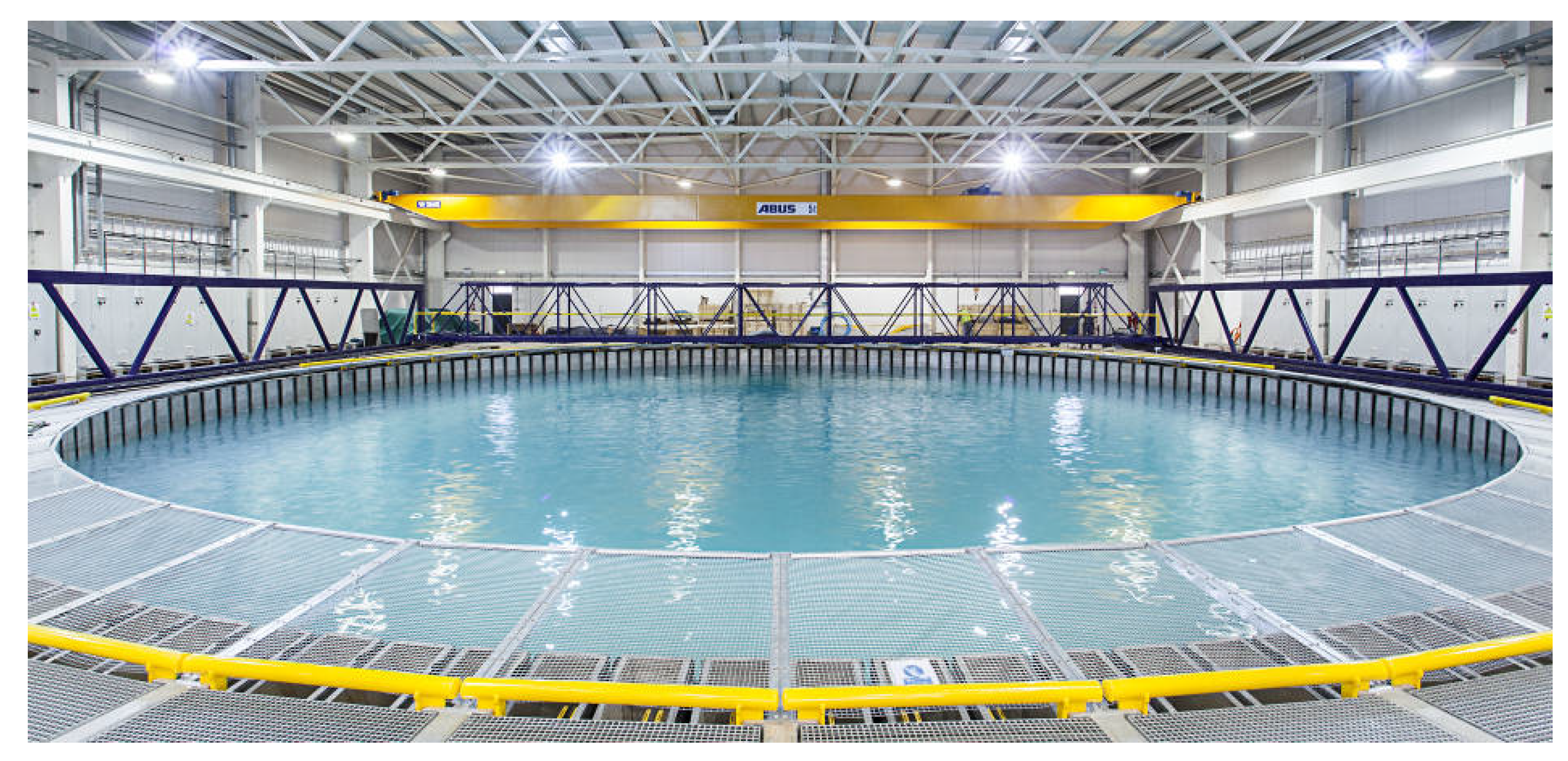
3.1. The FloWave Ocean Energy Research Facility

All experimental measurements presented here were made at the FloWave Ocean Energy Research Facility (Figure 2), based at the University of Edinburgh, U.K. [11]. The facility is a 25 m-diameter, circular, combined wave and current basin. Wave generation consists of 168 active-absorbing force-feedback wavemakers, with a nominal water depth of 2.0 m. A re-circulating flow system is implemented using 28 impeller units mounted in the plenum chamber beneath the floor [19]. These enable the creation of a predominantly straight flow in any direction across the central test area [20], where waves can also be added to the current field at any relative angle. A detailed drawing of the wave and current generation systems can be found in Sutherland et al. [13].

The nature of creating straight flow in a circular basin means that there is some inherent spatial variability [20]. Despite this, as a straight and uniform flow is largely achieved in the central test area, long-crested waves interacting co-linearly with the current field are still well approximated as long-crested. The same, however, cannot be said for the reflected waves. As shown in Draycott et al. [21], reflected waves are curved even without the presence of current due to the shape of the basin. Reflected waves are therefore only truly opposing the incident, as implied in Equation (9), along a centreline about the propagation direction. For this work, measurements are taken very close to this relative centreline (see Section 3.2.1 and Figure 3) where the influence of reflected wave curvature is negligible. As such, no modification to the theory presented has been implemented before application to data obtained from the FloWave tank.

3.2. Experimental Design

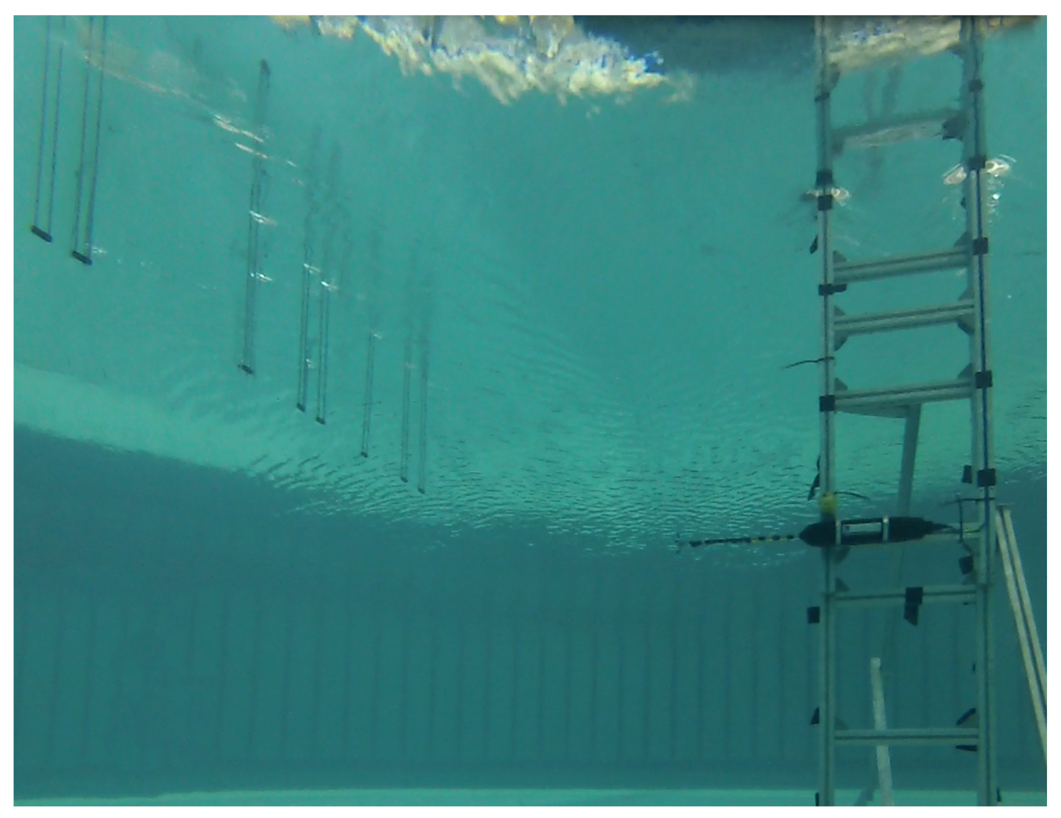
3.2.1. Instrument Configuration

Waves were measured using a linear array of seven multiplexed resistance-type wave gauges sampled at 128 Hz. Relative spacings were chosen to optimise reflection analysis performance and are detailed in

Table 1. Gauge x-positions.

Gauge Number	x Position (m)
1	2.016
2	1.854
3	1.583
4	1.258
5	1.150
6	0.879
7	0.338

. A Nortek “Vectrino” Acoustic Doppler Velocimeter (ADV) sampled at 100 Hz has been used to measure current velocity, which was mounted on a stiff slidable ladder structure. The two measurement systems are synchronised using a 5-V Transistor-Transistor-Logic (TTL) pulse from the tank generation software. The ability to slide the ADV enabled various z positions to be obtained and, hence, the assessment of the vertical decay of wave effects. The z-positions for the measurement volume of the ADV can be found in

Table 2. Acoustic Doppler Velocimeter (ADV) z-positions.

Position	z Position from Tank Floor (m)
1	1.77
2	1.57
3	1.27
4	0.97
5	0.37

.

Current velocity and wave spectra in current are spatially variable at FloWave, and as such, it is ideal to have the wave gauges and ADV in the same location. Due to installation constraints, this is not easily achievable, and so, an alternative approach was utilised. For collinear wave-current conditions, mirror symmetry is approximately observed at FloWave and, despite not providing time-domain equivalence due to turbulence, will provide equivalent average and spectral values between the two locations. The wave gauges and ADV were therefore placed at the same (but opposing) separation, S = 0.590 m, from the tank centreline. This is depicted in Figure 3, with an image from a video-camera installed on the tank floor presented in Figure 4.

3.2.2. Test Plan

In order to ensure the specified test conditions are realistic, site data have been utilised to identify common H-T-$\overrightarrow{U}$ (wave height-period-current velocity) combinations. For this work, data from the ReDAPT project (The Reliable Data Acquisition Platform for Tidal (ReDAPT) project was commissioned and co-funded by the Energy Technologies Institute (ETI), Loughborough, UK) [22,23,24,25] were utilised, which were obtained from the European Marine Energy Centre’s (EMEC) “Fall of Warness” grid-connected tidal test site. Full-scale equivalent velocities of 1.2, 1.8 and 2.4 m/s have been used with aligned waves of around 1-m significant wave height, $H_{m0}$. All sea states are defined using Pierson–Moskowitz (PM) spectra [26], as equivalent JONSWAP [27] peak-enhancement factors for the defined conditions were typically found to be close to unity.

The Mean Water Level (MWL) at the reference site is 45 m, and the tank is 2 m in depth; as such, a scale of 1:22.5 has been used throughout. Combined wave-current conditions have been Froude scaled to ensure full-scale similitude for the inertial and gravitational forces dominant in ocean waves. This results in tank-scale velocities of 0.25, 0.38 and 0.51 m/s. The Froude-scaled wave-current test conditions, reproduced at FloWave, are shown in

Table 3. Wave-current test plan for generation at FloWave. The 1:22.5 Froude scale compared with the Fall of Warness tidal test site. Each sea state is generated five times to measure at different depths with the ADV. Note that Reg. and Irreg. correspond to regular and irregular wave conditions respectively.

Sea State	Type	$\overline{\mathit{U}}$ (m/s)	${\mathit{H}}_{\mathit{in}}$ (m) (Reg.) or ${\mathit{H}}_{\mathit{m}0,\mathit{desired}}$ (m) (Irreg.)	T (s) (Reg.) or ${\mathit{T}}_{\mathit{p}}$ (s) (Irreg.)	Repeat Time, ${\mathit{T}}_{\mathit{R}}$ (s)	Run Time, ${\mathit{T}}_{\mathit{run}}$ (s)
1	Regular	0	0.049	1.6	8	64
2	Regular	0.25	0.049	1.6	8	64
3	Regular	0.38	0.049	1.6	8	64
4	Regular	0.51	0.049	1.6	8	64
5	Irregular	0.25	0.046	1.50	512	545
6	Irregular	0.38	0.049	1.50	512	545
7	Irregular	0.51	0.043	1.58	512	545

, noting that each sea state has been repeated five times to obtain the z-positions defined in Table 2. It is worth mentioning that there is no control over turbulence metrics or vertical profiles at the facility, and as such, only mean bulk flow is emulated. Turbulence Intensities (TI) at FloWave are typically between 5 and 10% [13]. For the three velocities used, 0.25, 0.38 and 0.51 m/s, the depth averaged TI values are 8.3%, 7.1% and 7.0%, respectively. Further specifics of the ADV analysis procedure, along with baseline (no waves) velocity and turbulence measurements, are given in detail in Sutherland et al. [13].

In order to have some simpler cases for analysis, regular waves (monochromatic) have been included in the test plan with comparable H and T values to the irregular sea states. Regular waves are not ‘corrected’ in current, and in Table 3, $H_{in}$ refers to regular wave heights input to the tank rather than what is produced at the measurement location, i.e., after interaction with the current field. For irregular seas, the spectra have been corrected in the presence of current to allow like-for-like comparisons with site data for other parts of the FloWTurb project. $H_{m0,desired}$ is the target significant wave height, where actual measured $H_{m0}$ values are very close to desired, as demonstrated in Section 4.1 (Figure 5).

4. Results and Discussion

This section details and discusses the results of the experiments. The corrected irregular sea states are briefly shown in Section 4.1. The effect of current on waves is explored in Section 4.2, where wave height modification by current and the current influence on the stationarity and repeatability of wave conditions is assessed. Section 4.3 shows outputs of the wave reflection analysis procedure. Section 4.4 compares the predicted wave-induced particle velocities from the reflection analysis to the ADV measurements and shows the decay of wave-induced current effects with depth.

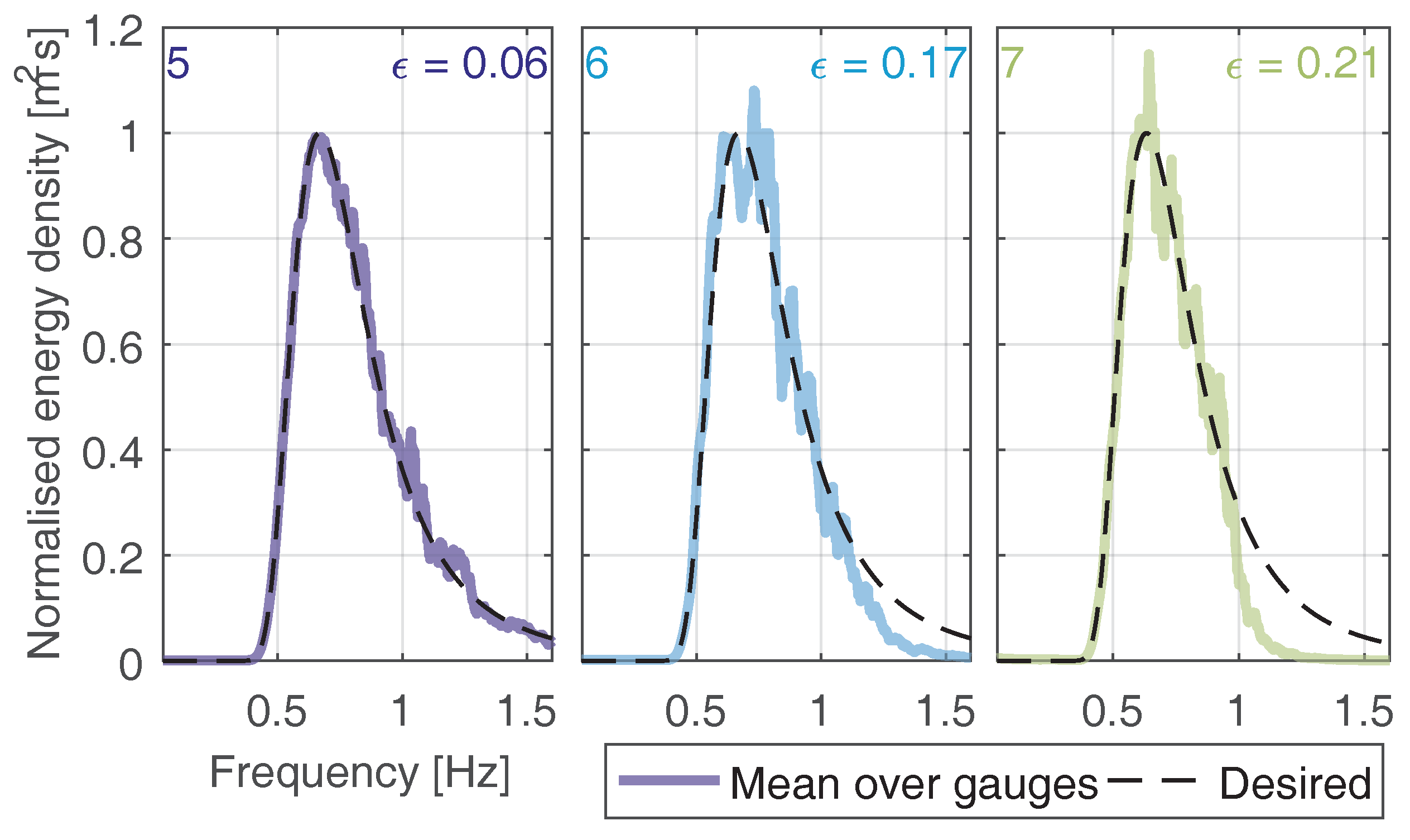
4.1. Corrected Irregular Sea States

As mentioned in Section 3.2.2, it was desired to obtain ‘corrected’ wave spectra for the irregular sea states defined in Table 3. Due to the interaction with the current field, wave amplitudes are not as specified and require correction. Linear frequency-dependent correction factors are calculated via Equation (18). In this case, $A_{i,measured}$ is defined as the mean spectrum over the gauges obtained from an FFT. The error between target spectrum and measured is calculated from Equation (19).

$$CF(f_i,{\theta }_i)=\frac{A_{i,desired}}{A_{i,measured}}$$

(18)

$$\epsilon =\frac{{\sum }_{i=1}^{N_f}\left|S_{measured}\left(f_i\right)-S_{desired}\left(f_i\right)\right|}{{\sum }_{i=1}^{N_f}{S}_{desired}\left(f_i\right)}$$

(19)

The linear correction factors were applied iteratively to the input amplitudes (compounded) up to a maximum of three iterations. The final corrected mean spectra are shown in Figure 5 with corresponding resulting errors. Note that there was some difficulty in generating large enough high frequency wave components in the higher current velocities. This is a combination of frequency-dependent paddle limits and the larger following currents reducing wave amplitudes significantly. Despite this, it is evident that the mean spectra are very close to the desired. This is especially true for regions around the peak frequency, where the higher energy components of greater interest lie. As discussed in Section 4.3, however, point measurements and incident spectra can differ significantly.

To ensure the correct current velocity, previous depth averaged calibrations have been used to set tank flow-generation motor RPM (as presented in [13]). These were verified with the ADV in situ to ensure that they were still valid at the measurement location. As mentioned in Section 3.2.2, it is only possible to control the flow speed and direction, and as such, the resulting turbulence statistics and depth profiles will differ from full-scale site equivalents. Details of flow characteristics can be found in Sutherland et al. [13].

4.2. Effect of Current on Waves

The outputs of the tests allow some assessment of the influence of current on the waves at FloWave. This includes modification of the key wave parameters themselves, in addition to the effect of turbulence on wave repeatability and the assumption of stationarity.

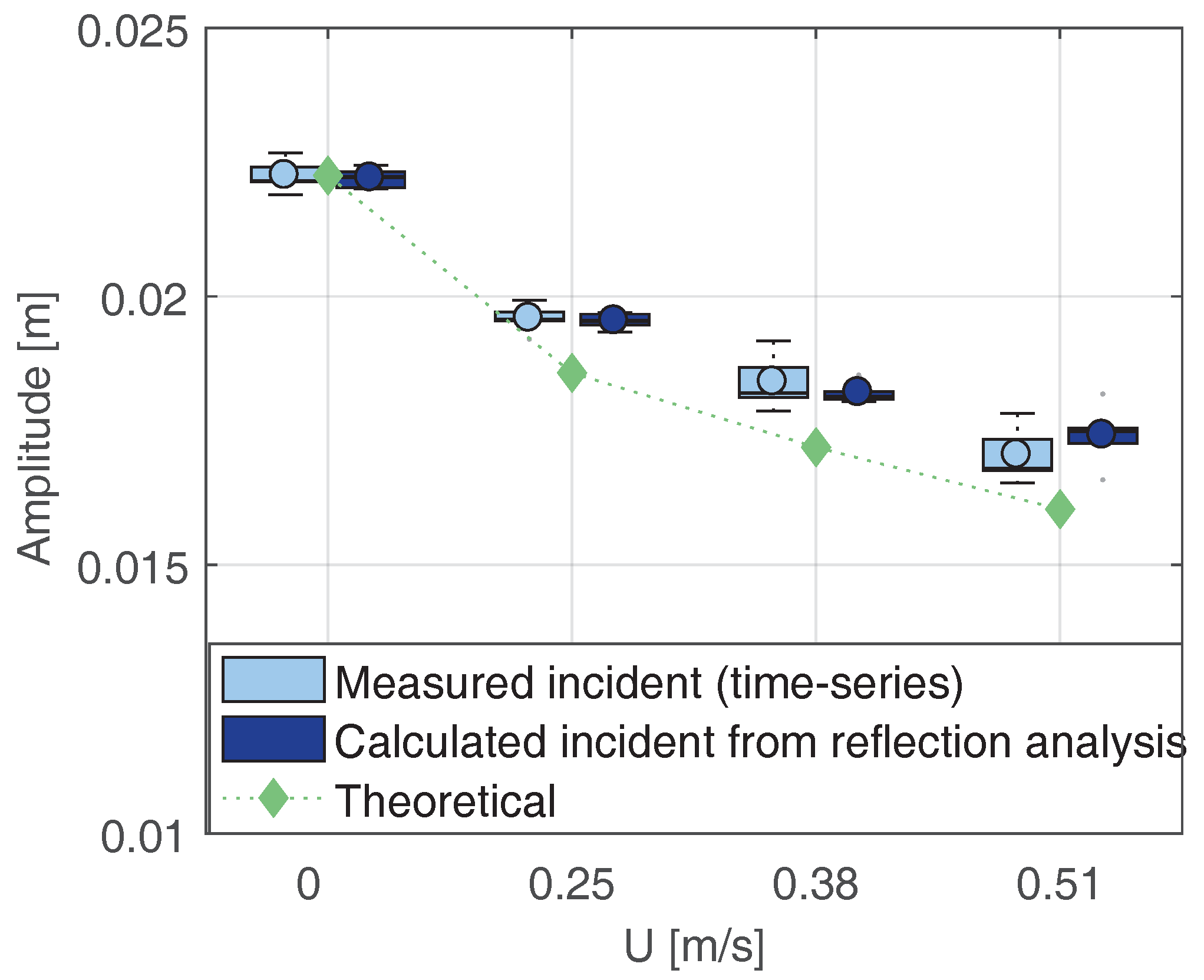
4.2.1. Wave Height Modification by Current

The modification of wave height by current can be approximated by Equation (5). All regular wave cases generated had the same input H and T values, and as such, the influence of current on wave properties at FloWave can be easily isolated. Figure 6 shows the incident regular wave amplitude compared with the theoretical change computed using Equation (5). This has been calculated in two ways: using the frequency-domain reflection analysis procedure described in Section 2.2.1 and utilising a time-domain approach. The time-domain method only uses the first portion of the time series, unaffected by reflection, and applies a zero down-crossing analysis to obtain an estimate of the incident wave amplitude. The frequency-domain method presented (Section 2.2.1) is applied to the last section of the data where reflections are built up and stationarity is a reasonable assumption. For this work, the last 16 s of data were used, which represents an apparent period of stationarity for all current velocities. An example time series is shown in Section 4.2.2 (Figure 7), which serves as a good example for why this is required.

From Figure 6, it is evident that the two approaches of estimating the incident wave amplitudes agree well with each other. This serves as a good proof of the reflection analysis method in combined wave-current and gives confidence in the application to irregular sea states. It is also clear that decreased repeatability is observed in higher current conditions, indicated by the larger inner quartile range of the box plots. This is discussed further in Section 4.2.2.

The theoretical modification of wave height by current in these conditions, re-produced at FloWave, seems to slightly over-estimate the influence of current on the wave height. However, in Draycott et al. [17], it is suggested that the tank wave generation may respond to the presence of current and as such may be a tank-specific effect, rather than inaccuracies in the theory. It is also noted that wavelength predictions for waves in current appear to be correctly predicted in FloWave by Equation (2) [17], which will also be true for other facilities. Additionally, it is likely that other tanks will experience n analogous response from wavemakers to the direct and indirect effects of the current generation. Importantly, for the method presented in Section 2, incident and reflected wave amplitudes are solved for, and as such, any facility-specific wavemaker response to current will not affect the accuracy of results.

4.2.2. Repeatability and Stationarity

Fluctuations in the current velocity introduced by turbulence cause temporally-variable wave modification by the current. This causes a decrease in the repeatability of the wave measurements and introduces uncertainty in the assumption of stationarity inherent to spectral analysis methods. The other cause of non-stationarity is the presence of reflections, which are not present at the start of a test, but appear some time, $t_{refl}$, during the measurement. $t_{refl}$ is a function of the wave frequency and current velocity.

Both the repeatability issue from turbulence and stationarity issues with reflections are well demonstrated for both regular and irregular waves in Figure 7 and Figure 8, respectively. In Figure 7, five repeats are overlaid for Sea State 2, and two gauges, 2 and 7, are shown. The time at which amplitude readings for Gauges 2 and 7 diverge shows the point where reflections are present at the array location, causing spatially-dependent interference. It is evident that despite the non-stationarity for the overall test, there is a period of stationarity with just the incident wave train (approximately 15–35 s) and a period of stationarity where reflections have built up beyond $t_{refl}$ (approximately 40–64 s). These correspond to the two different regions used in Section 4.2.1 to obtain time- and frequency-domain estimates for the incident wave amplitudes.

For the regular wave case (Sea State 3) shown in Figure 7, it is evident that the repeatability is high. However, for the equivalent example in irregular waves (Sea State 6), Figure 8, this is not the case, and the repeatability is significantly worse. This is a result of the presence of high frequency components. The higher frequency waves, with lower $C_g$, are significantly more affected by the current velocity and associated turbulent fluctuations. A summary of the repeatability is shown in

Table 4. Repeatability of waves and current. Mean coefficient of determination, $r^2$, shown for each test. Averaged over all repeats compared to all other repeats and over all gauges. Sea state references correspond to those defined in Table 3.

Sea State	1	2	3	4	5	6	7
$r^2$	0.994	0.993	0.988	0.931	0.691	0.592	0.522

. The coefficient of determination, $r^2$, is used as the repeatability metric. $r^2$ values are computed between all repeats, and the mean value over all gauges is presented. It is apparent from Table 4 that high repeatability is observed for all the regular wave cases, yet relatively poor repeatability is associated with the irregular sea states. As expected, the repeatability worsens significantly in increased current conditions.

4.3. Separating Incident and Reflected Waves

This section presents the results of the wave reflection analysis procedure described in Section 2.2.1. The incident and reflected wave spectra are presented in Section 4.3.1, which demonstrates the reflection method and shows how reflection characteristics at FloWave differ in current. In Section 4.3.2, time series of wave surface elevations are estimated from the method and compared with gauge data. This is carried out to demonstrate that wave elevations at various positions can be estimated from the isolated wave systems, which means that wave-induced velocities should also be possible to predict.

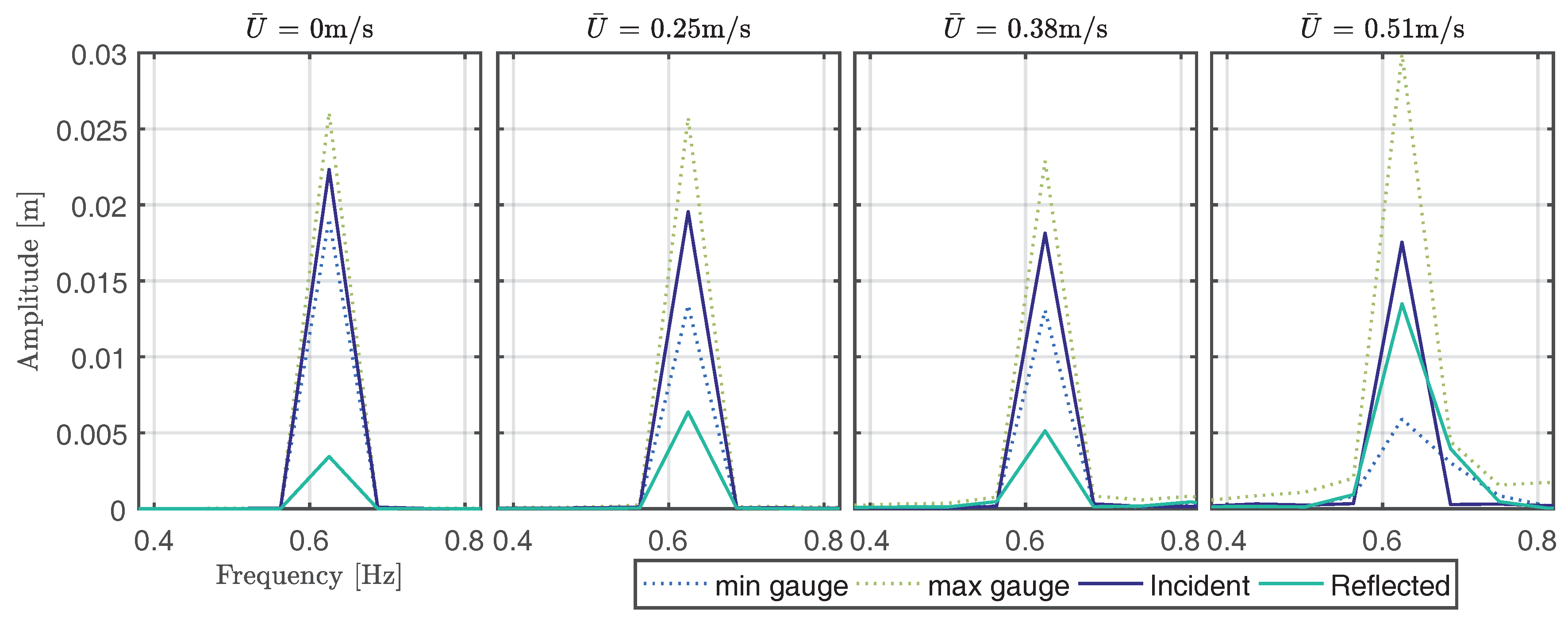
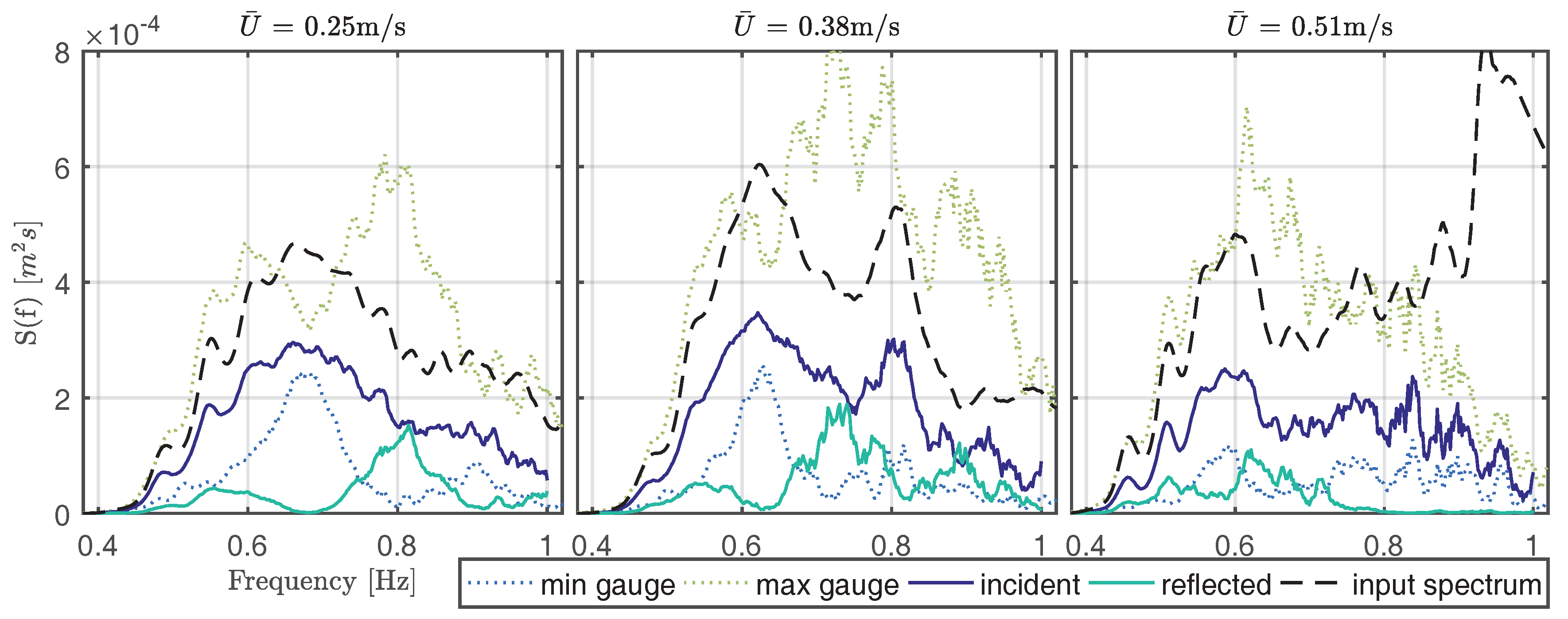
4.3.1. Isolation of Incident and Reflected Spectra

The reflection analysis procedure (Section 2.2.1) has been applied to the sea states defined in Table 3. Only the final 16 s of regular wave cases and final 512 s of irregular wave cases were used to ensure that the assumption of stationarity is as reasonable as possible (see Section 4.2.2). These correspond to integer multiples of the repeat time (see Table 3), in order to have output frequencies from an FFT that correspond to tank generation frequencies.

The resulting incident and reflected spectra for the regular wave cases (Sea States 1–4) are shown in Figure 9. It is noticeable from this figure that the reflections are larger in increased following currents at FloWave. This is partly a result of reflected waves interacting with a larger opposing current, hence increasing in amplitude. It is also known, however, from Draycott et al. [17] to be partly a result of poorer absorption performance of the force-feedback wave paddles in current. The minimum and maximum amplitudes measured over the wave gauge array are also shown in the Figure 9, and it is clear that reflections introduce significant spatial variability in the wave field in high current conditions.

The isolated incident and reflected amplitude spectra for the irregular wave cases (Sea States 5–7) are shown in Figure 10. In order to obtain the corrected mean spectra over the array, Figure 5, it is clear that input, and resulting incident wave spectra, are not characteristic of Pierson–Moskowitz-defined sea states. The input spectrum, also shown on the graphs, shows that the calculated incident spectrum is as expected, containing the details defined in the input spectrum. This demonstrates the effectiveness of the reflection analysis methodology. The incident spectra appear as a scaled-down version of the input spectrum due to interaction with the following current field.

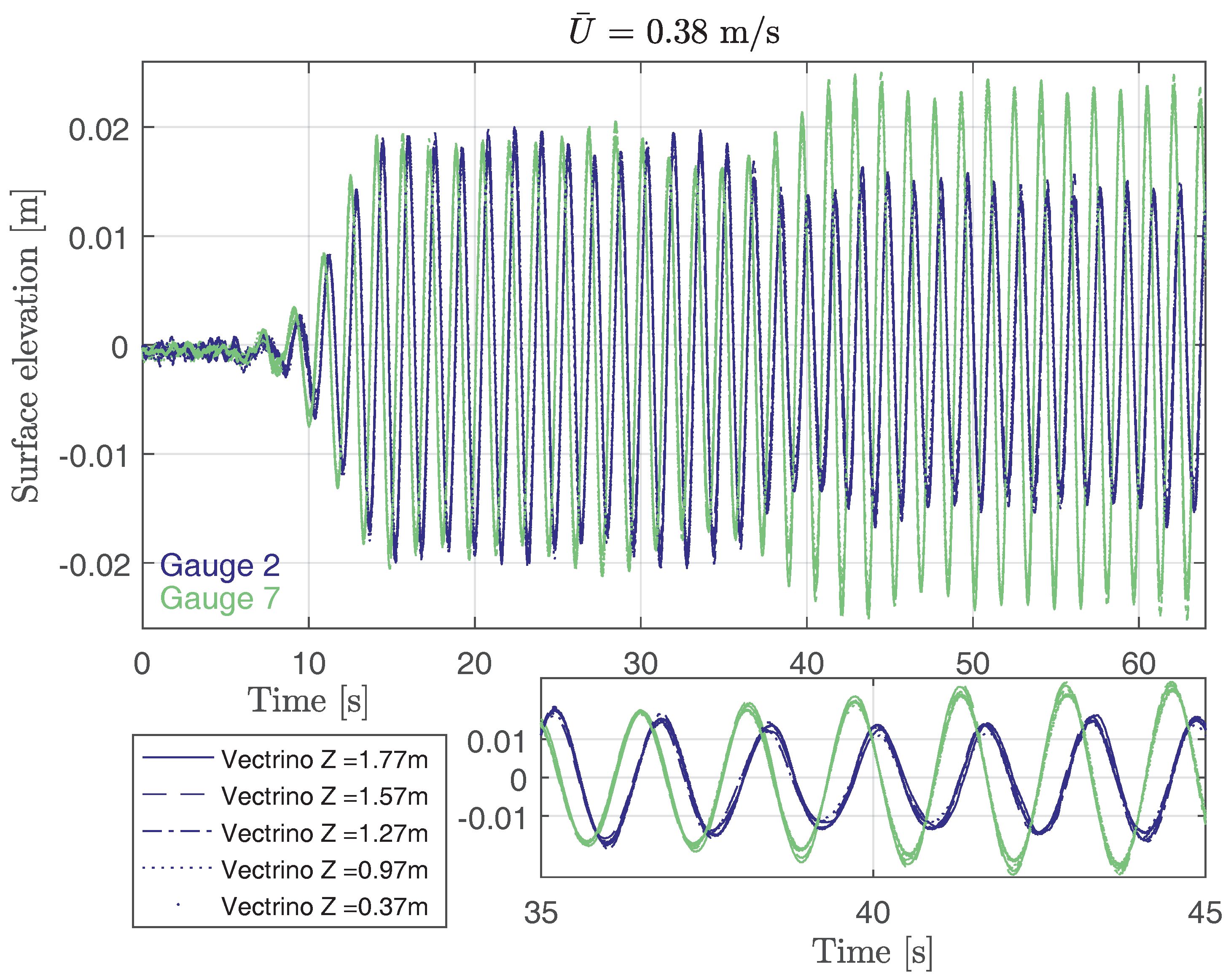
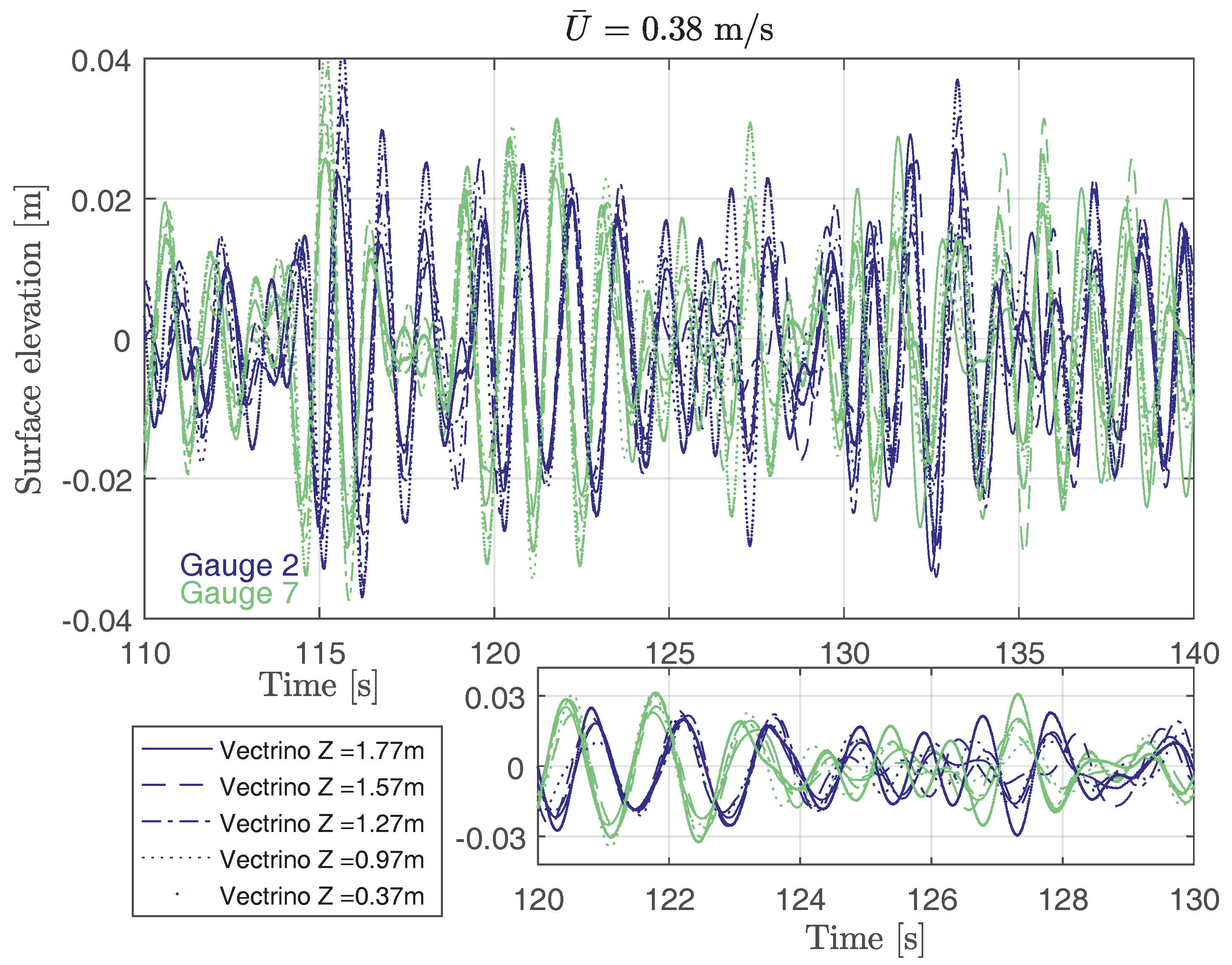
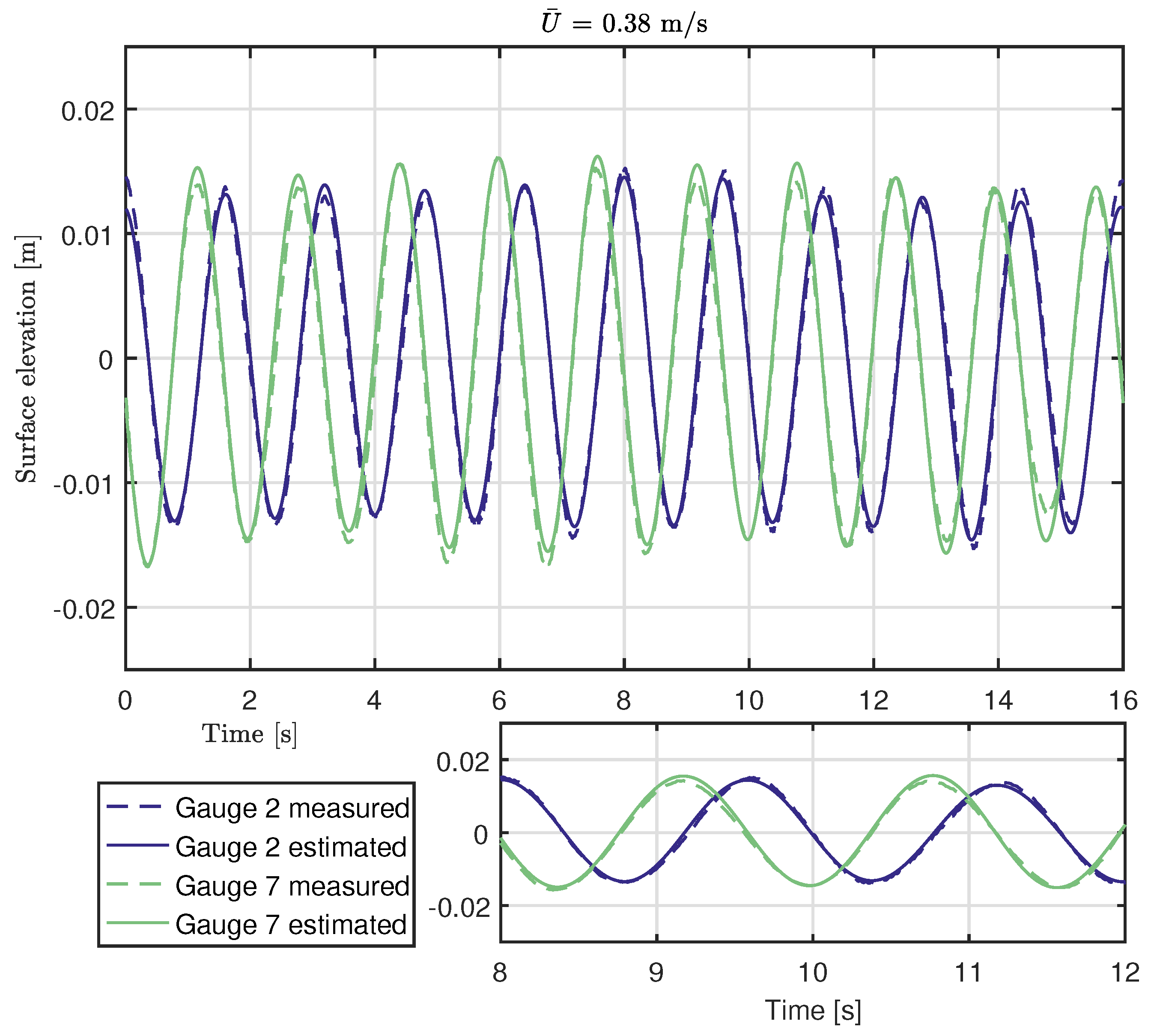
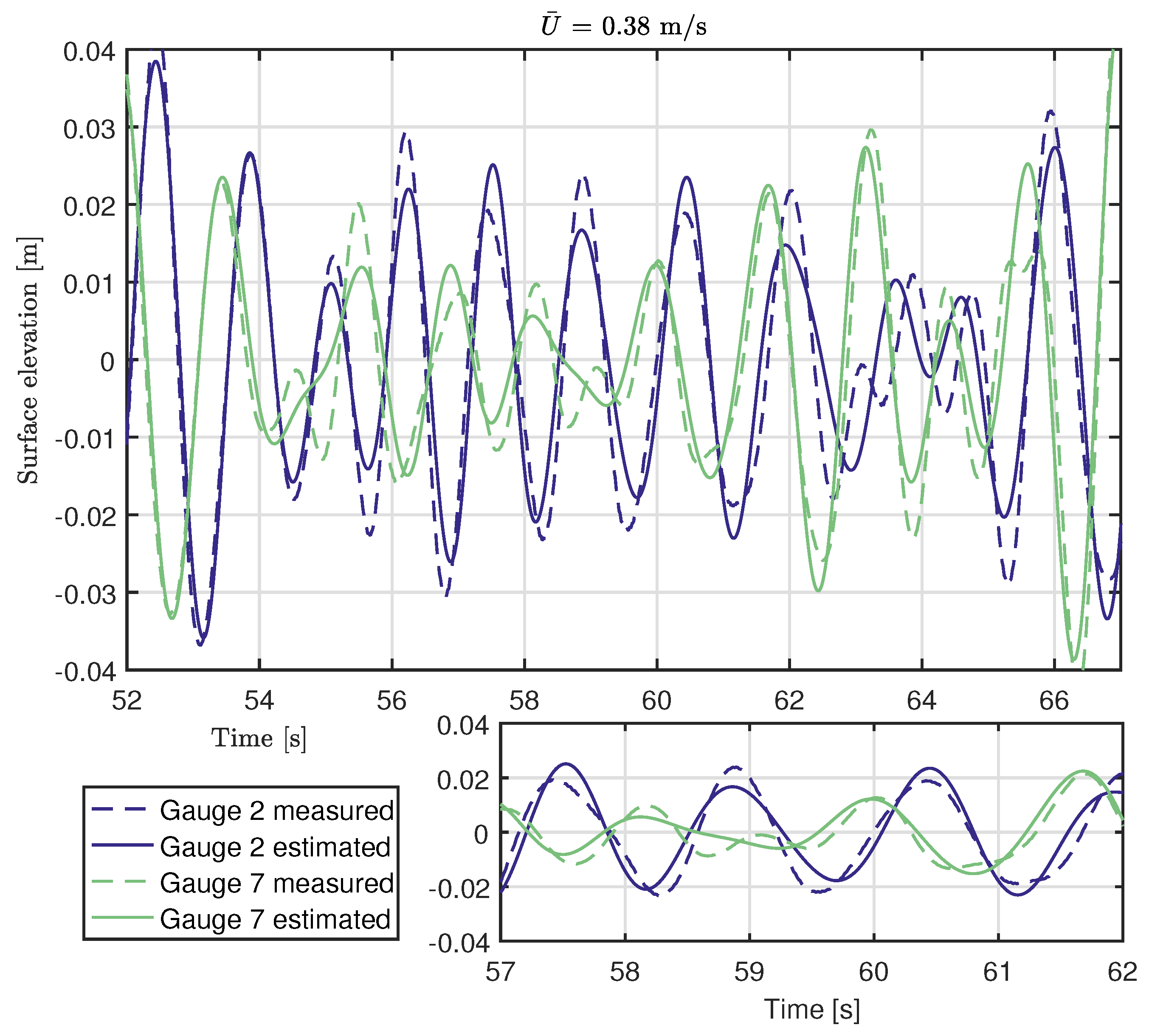
4.3.2. Prediction of Time Series

The outputs of the reflection analysis procedure (Section 2.2.1) essentially provide complex incident and reflected amplitude spectra, $a_{inc}$ and $a_{ref}$. As the phase is preserved, it is possible to simulate the expected total time series at any x-position and, hence, validate against the measured data at the various gauge positions. In each case, the phase that is incorporated into the complex values is relative to x = 0 m, and as such, they need to be shifted to the gauge x-positions defined in Table 1 for comparison. This can be done in a similar manner as is described for velocity spectra in Equations (16) and (17). Applying an Inverse Fast Fourier Transform (IFFT) to the transformed spectra provides the expected time series at the gauge positions. Examples for regular and irregular sea states are displayed in Figure 11 and Figure 12, respectively. As in previous examples, the 0.38-m/s current cases are used, and Gauges 2 and 7 are displayed. Repeat 3 is shown; however, the results are extremely similar for each of the five repeats (ADV z-positions).

From Figure 11 and Figure 12, it is clear that the reflection analysis methodology has worked well, and the incorporated and transformed phases are good approximations despite the non-stationarity introduced by turbulence. It can be further confirmed from this that the estimations of wavenumber in current are reasonable, Equation (2). A summary of the time series estimation performance for all sea states, and averaged over all gauges, is shown in

Table 5. Time series simulation from reflection analysis vs. measured time series. Mean coefficient of determination, $r^2$, shown for each test. Averaged over all gauges and all repeats. Sea state references refer to those defined in Table 3.

Sea State	1	2	3	4	5	6	7
$r^2$	0.994	0.996	0.984	0.914	0.781	0.816	0.884

. Reasonably good estimations are found for all sea states. Regular wave cases display the expected trend, with the estimations becoming worse in higher current; however, the opposite is observed for the irregular sea states. This is likely due to phase errors in the high frequency components, whereby a smaller proportion of the high frequency content is present in the higher velocity conditions, as shown in Figure 5. Overall, however, confidence is gained in the procedure for isolating incident and reflected wave spectra and predicting observations at a given location. This gives confidence that the same will be true for predicting water particle motions, as described in Section 2.2.2. Results of this are shown in Section 4.4.

4.4. Wave-Induced Particle Velocities in Combined Wave-Current Fields

Without knowledge of the incident and reflected wave spectra, and a frequency-dependent phase relationship between them at a given position, it is not possible to estimate the wave-induced velocities. Once the two systems are well defined, it is possible to estimate the horizontal and vertical particle velocities through Equations (14)–(17) and compare with measurements. The results of this are shown for the regular and irregular sea states in Section 4.4.1 and Section 4.4.2, respectively.

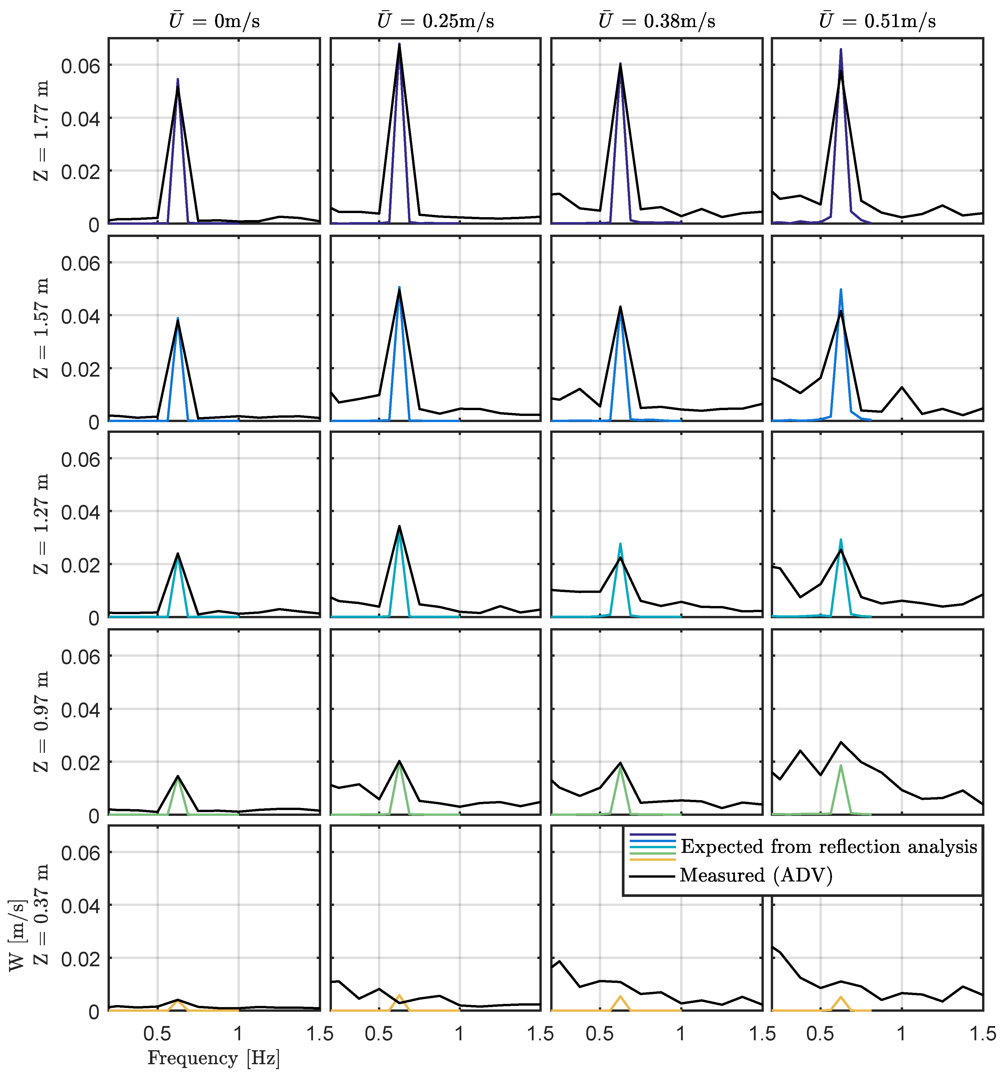
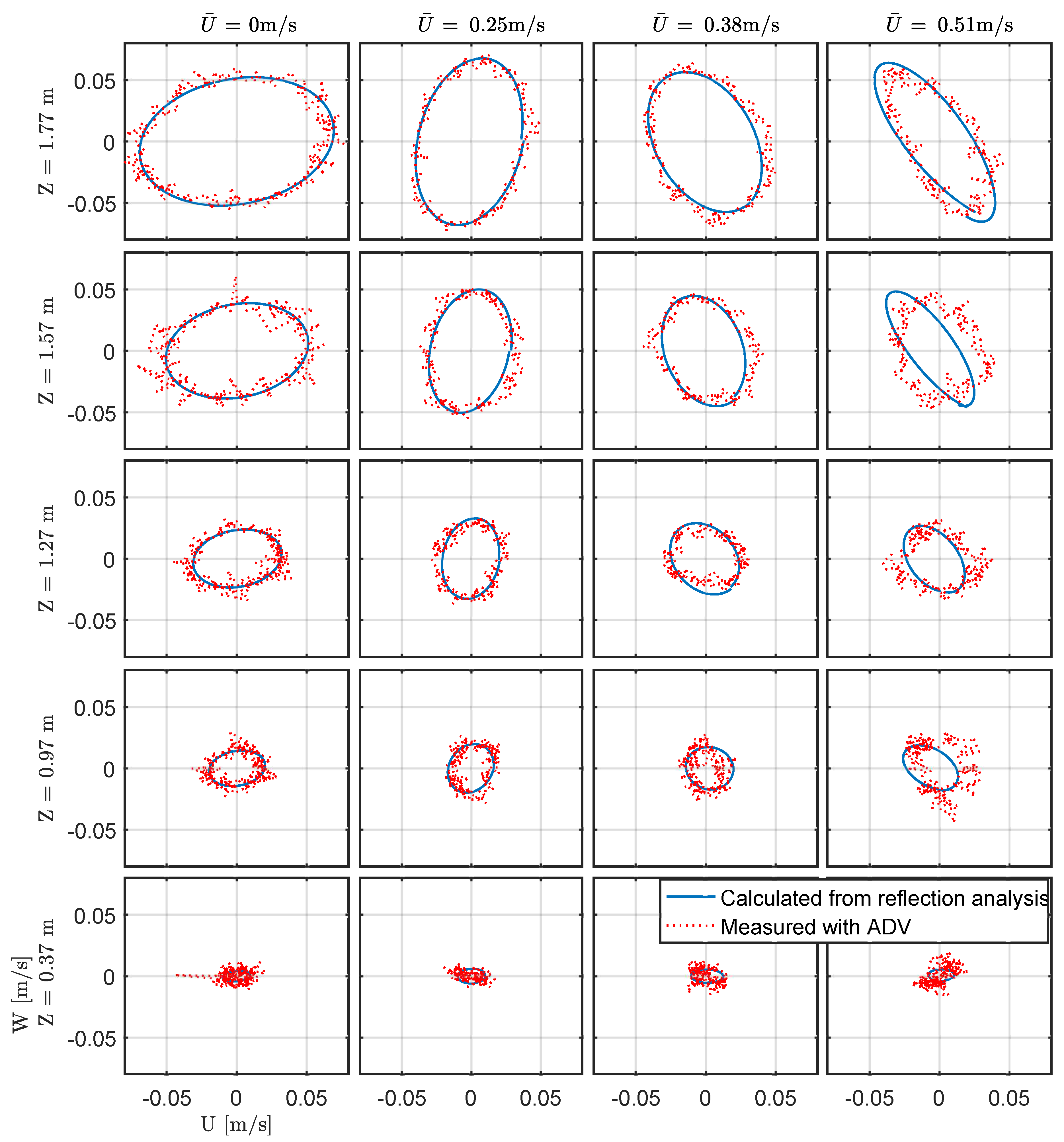
4.4.1. Regular

The predicted horizontal U, and vertical, W, velocity spectra compared with the measured equivalents from the ADV are shown in Figure 13 and Figure 14, for Sea States 1–4 at each of the five depths. As these are monochromatic sea states, the FFT has been applied so that the wave energy all lies within a single frequency bin. This allows for fair comparison. It is evident that the estimates are overall very good, with slightly larger deviations observed in higher velocity conditions further down in the water column.

Without obtaining the correct phase relationship between the incident and reflected spectra, the estimated velocity magnitudes would display large deviations from the measured equivalents. This would make it difficult to validate the application of linear wave theory in these sea states. The spatially-variable relationship between incident and reflected waves also causes deviations from the typically expected wave orbital motions, which are shown via the relationship between U and W velocities. This can be predicted by simulating time series of U and W over an individual wave period. This is shown in Figure 15 compared with the measured equivalent. With the aim to remove the influence of turbulence, the measured equivalent is taken as the average ‘orbital’ over the last 16 s, i.e., the mean of exactly 10 wave cycles at T = 1.6 s.

It is discernible from Figure 15 that reflections are greatly altering the wave orbitals and that this change is largely predictable from the theory detailed in Section 2.2.1 and Section 2.2.2. The exception may be the 0.51 m/s case, where for 1.57 m, there is clear disagreement. Interestingly, for most predictions at 0.51 m/s, expected orbitals are also not a closed loop, which is attributed to the effect of unexpected frequency components present in the wave analysis. Nevertheless, this diagram therefore serves as a nice proof of the method and shows that some of the complexities in wave-induced particle velocities with reflection are predicable with linear wave theory. Importantly, this ability to include tank reflection also gives the possibility to remove its influence from the results if trying to assess full-scale behaviour (without tank reflection).

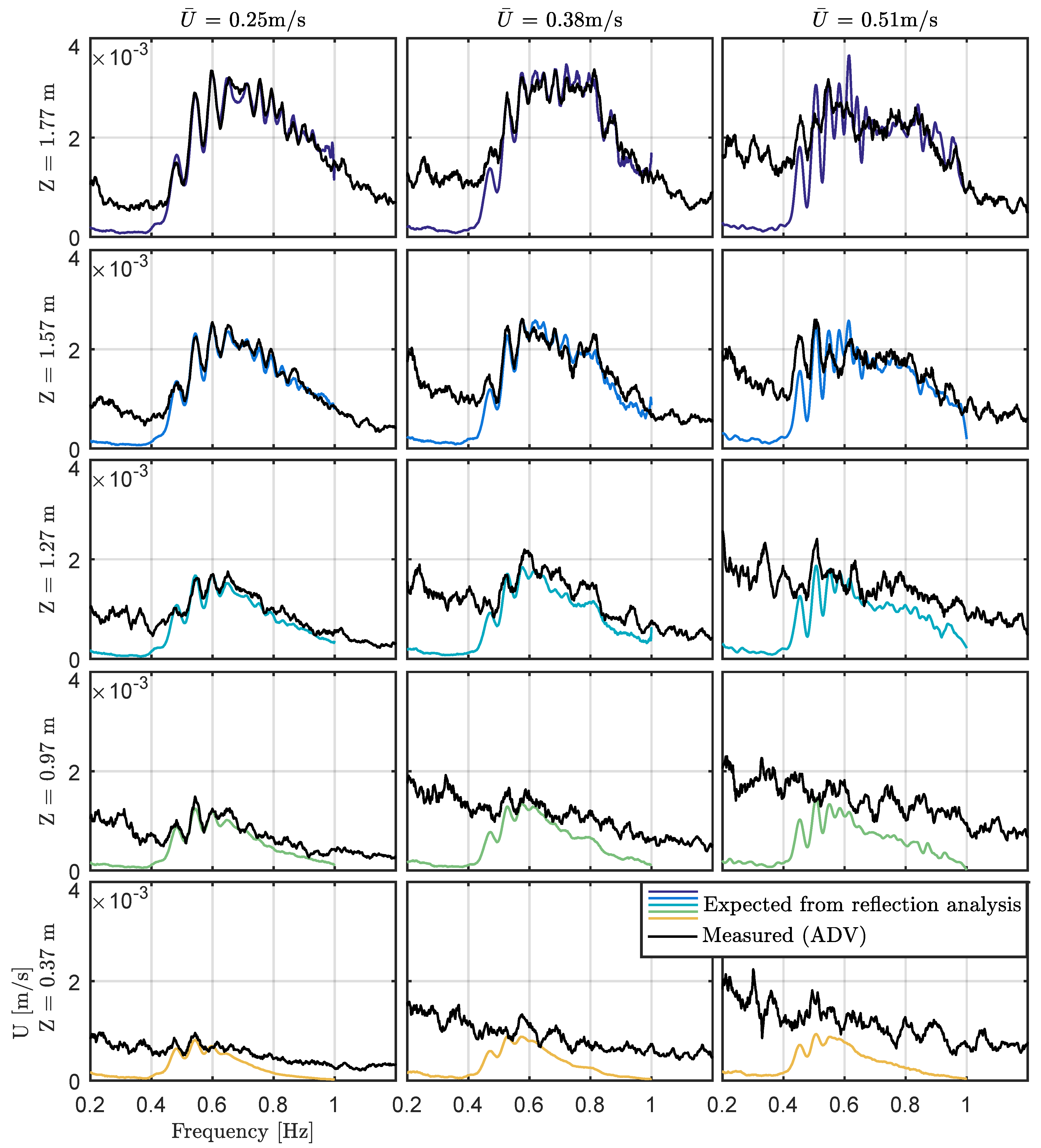
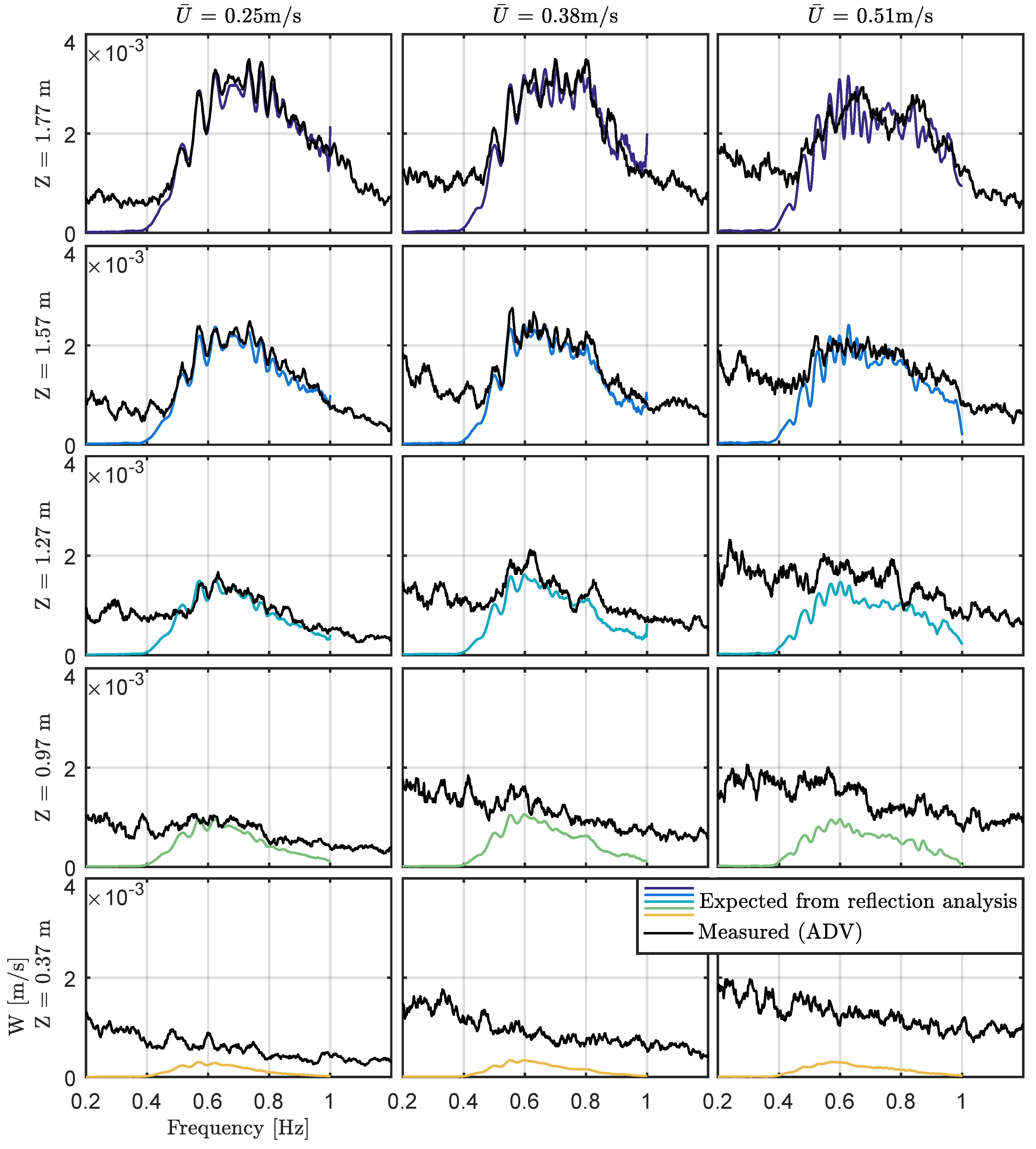
4.4.2. Irregular

The velocity spectra for irregular waves, compared with those expected from the wave analysis, are shown in Figure 16 and Figure 17. Similarly, it is observed that the estimates are very close to the measured spectra, with slightly worse results detectable for the 0.51-m/s case. The ‘spiky’ variation observed is due to the ADV being at constructive and destructive interference locations, which is a function of frequency. A destructive location in U for a given frequency is a constructive point for W and vice versa, i.e., partial standing waves are formed. The estimated wave-induced velocity spectra are extremely similar to the measured and describe the interference-induced variations very well. Interestingly, for both the regular and irregular sea states, it appears that the wave surface elevations alone can be used to predict the velocities across the relevant wave frequencies. This is particularly true for low to medium-high current velocities and reasonably valid for high current velocities higher up in the water column. This suggests that wave effects are dominant in these conditions.

5. Implications of Findings

As there are a variety of interesting elements to the results, a summary of the main findings is presented here in relation to the four areas detailed in the Introduction (Section 1):

• Ability of linear wave theory, with reflection analysis, to predict wave-induced particle velocities:
  It is clear that the theory presented in Section 2 is able to predict the wave-induced velocities for low to medium-high current velocities, including the accurate prediction of wave orbital motions. This is applied to the 0.25-m/s and 0.38-m/s cases corresponding to 1.2 m/s and 1.8 m/s full scale. For waves in very large currents, 0.51 m/s tank scale (2.4 m/s full scale), the theory still provides useful estimates, but is notably less accurate. This is likely due to calculations being carried out in the frequency-domain and the inherent assumption of stationarity no longer being a good approximation.
  This ability to predict the wave-induced velocities for the more complex situation of having significant wave reflection present gives confidence that it can be applied when there is no reflection, e.g., in numerical models or when analysing site data. It also enables the attribution of velocities induced by wave reflection and gives the ability to compensate or remove these components from key test outcomes that are dependent on velocity, e.g., turbine power fluctuations or blade bending moments.
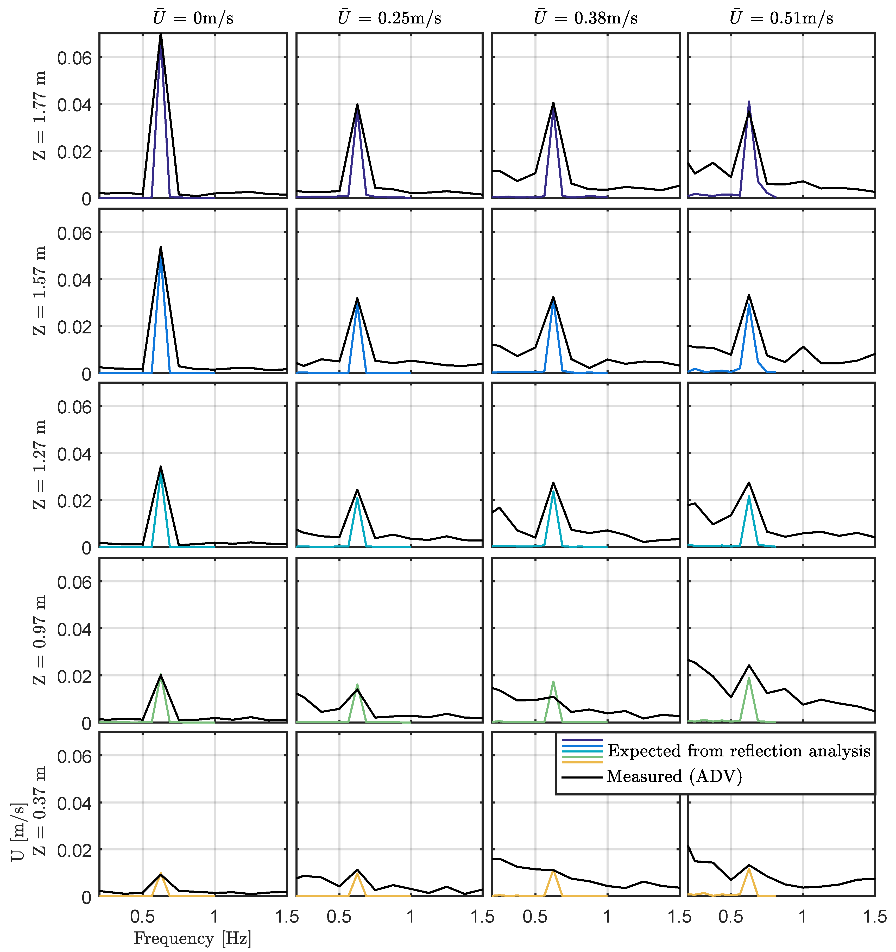
• Experimental results of wave-induced particle velocities with depth:
  The results of velocity spectra with depth reveal two essential points. First is that linear wave-current theory can be used to predict the decay of waves with depth fairly accurately, particularly for lower flow conditions. Second is that for low to medium-high current velocities, the wave effects completely dominate the velocity fluctuations in the upper region of the water column. Expected wave-induced velocities alone can be used to predict the energy content, and it appears that underlying turbulence at these frequencies becomes insignificant. There is a limitation to this, which is evident in the data: for waves that are higher frequency, lower amplitude and measured lower in the water column, this statement will be less appropriate. In addition, turbulence will dominate at the bottom boundary due to the significance of turbulence-generating mechanisms relative to the influence of highly attenuated waves.
• Effect of current on the wave field:
  The current is found to affect the wave field in a number of ways. Current alters the form of the waves, including wave height and wavenumbers, but also alters a number of other aspects of wave statistics. Turbulent fluctuations cause a significant decrease in stationarity, as the changes in velocity alter the amplitudes and phases of measured wave components. For tank tests, this decreases repeatability, which is worsened in larger currents and when there is significant high frequency wave content. At FloWave, the presence of current also increases wave reflection, which is time-varying and further reduces the assumptions of stationarity. This aspect, however, can be overcome by choosing a time-section when reflections are both present and stable.
• Issues with re-creating combined wave-current conditions in test tanks:
  In addition to the issues of stationarity and repeatability summarised in point 3 (above), there are other issues with re-creating site wave-current conditions in test tanks. One such issue is dealing with the presence of reflections, discussed in detail in this paper. Reflections cause mean spectra over an array of gauges to differ significantly from the incident spectra. Mean spectra were used for corrections in this case; yet, even if incident spectra were corrected, the vertical and horizontal velocities will differ notably from site data due to the presence of reflections. This is evident from Figure 16 and Figure 17 where essentially this ‘spiky’ variation in the spectra is unavoidable.
  Another issue, touched upon in Section 3.2.2 and Section 4.1, is that there is not much control over the nature of the current other than its principal direction and speed. Matching turbulence statistics or depth profiles to site equivalents was not possible at FloWave and is typically not achievable in any of the larger test facilities. The nature of the turbulence will have significant implications of TST loads and performance [28] and as such remains a major challenge if true similitude to site wave-current conditions is to be attained. It is, in certain facilities, possible to deploy turbulence-modifying grids as detailed and discussed in [29,30,31], and this approach has been used to vary turbulence in test conditions for TSTs [28,32]. This, however, is typically much easier to achieve in small tanks and flumes. For larger facilities, the potential size of grids poses a practical challenge, along with the effect of flow diversion if only locally deployed. For FloWave, a large basin of circular geometry, a system has yet to be developed.
  The results presented in this paper are all for uni-directional waves in collinear following currents. In the real world, however, wave conditions may be significantly directionally spread and may propagate at various angles to the current field. This directionality has the potential to significantly alter the loading on a device and as such is an important aspect to consider. At present, however, in order to accurately reproduce and characterise these more complicated directional wave-current conditions, additional measurement and analysis techniques are required. It is necessary to resolve incident and reflected component wave angles in addition to amplitudes, which is thought possible through the extension of the least-squares approach presented. At present, however, this remains an element for further work.

6. Conclusions

Waves are a major contributor to unsteady loads on tidal turbines, and as such, the wave-current environment is important to understand and test tidal turbines within. To this end, a variety of high current conditions, ranging from 1.2–2.4 m/s full-scale equivalents, have been specified and re-produced with selected wave cases at FloWave. The ability of linear wave theory to predict the wave effects in large currents is tested, along with focussing on the effect current has on the wave field in the tank and the issues this introduces.

It is found through the tank tests that linear wave theory, combined with reflection analysis, is able to predict the wave-induced velocities well for low to medium-high currents and provides reasonable estimates for high current velocities. Stationarity and repeatability are significantly worsened when current is increased, and the validity of spectral analysis methods at high velocities becomes questionable. It is concluded that this is a result of increased turbulent fluctuations at higher current introducing a temporally-variable and unpredictable wave-current interaction.

The results presented further understanding on testing in the complex wave-current environment, along with the validity and limitations of linear wave theory. In addition, the analysis tools presented will enable more effective understanding of complex wave-current conditions in the tank environment and will help in the isolation of tank effects from identified full-scale conditions.

References

- Carbon Trust. UK Tidal Current Resource and Economics Study. 2011. Available online: https://www.carbontrust.com/media/77264/ctc799_uk_tidal_current_resource_and_economics.pdf (accessed on 27 September 2017).
- Black&Veach. Technical Report: Phase II. UK Tidal Stream Energy Resource Assessment. Available online: https://www.carbontrust.com/media/174041/phaseiitidalstreamresourcereport2005.pdf (accessed on 27 September 2017).
- Atlantis. MeyGen | Tidal Projects | Atlantis Resources. Available online: https://www.atlantisresourcesltd.com/projects/meygen/ (accessed on 1 August 2017).
- Milne, I.A.; Sharma, R.N.; Flay, R.G.J.; Bickerton, S. The Role of Waves on Tidal Turbine Unsteady Blade Loading. In Proceedings of the 3rd International Conference on Ocean Energy, Bilbao, Spain, 6–8 October 2010; pp. 1–6. [Google Scholar]
- Faudot, C.; Dahlhaug, O.G. Prediction of wave loads on tidal turbine blades. Energy Procedia 2012, 20, 116–133. [Google Scholar] [CrossRef]
- Luznik, L.; Flack, K.A.; Lust, E.E.; Taylor, K. The effect of surface waves on the performance characteristics of a model tidal turbine. Renew. Energy 2013, 58, 108–114. [Google Scholar] [CrossRef]
- Fulton, J.; Luznik, L.; Flack, K.; Lust, E. Effects of waves on BEM theory in a marine tidal turbine environment. In Proceedings of the OCEANS’15 MTS/IEEE, Washington, DC, USA, 19–22 October 2015. [Google Scholar]
- Tatum, S.C.; Frost, C.H.; Allmark, M.; O’Doherty, D.M.; Mason-Jones, A.; Prickett, P.W.; Grosvenor, R.I.; Byrne, C.B.; O’Doherty, T. Wave-current interaction effects on tidal stream turbine performance and loading characteristics. Int. J. Mar. Energy 2016, 14, 161–179. [Google Scholar] [CrossRef]
- EPSRC. FloWTurb: Response of Tidal Energy Converters to Combined Tidal Flow, Waves, and Turbulence. Available online: http://gow.epsrc.ac.uk/NGBOViewGrant.aspx?GrantRef=EP/N021487/1 (accessed on 15 August 2017).
- FloWTurb. FloWTurb Research Group Home page | FloWTurb Research Group. Available online: http://www.flowturb.eng.ed.ac.uk/ (accessed on 1 August 2017).
- Ingram, D.; Wallace, R.; Robinson, A.; Bryden, I. The design and commissioning of the first, circular, combined current and wave test basin. In Proceedings of the Oceans 2014, Taipei, Taiwan, 7–10 April 2014. [Google Scholar]
- Holmes, B. Tank Testing of Wave Energy Conversion Systems. Available online: http://www.emec.org.uk/tank-testing-of-wave-energy-conversion-systems/ (accessed on 27 September 2017).
- Sutherland, D.R.J.; Noble, D.R.; Steynor, J.; Davey, T.A.D.; Bruce, T. Characterisation of Current and Turbulence in the FloWave Ocean Energy Research Facility. Ocean Eng. 2017, 139, 103–115. [Google Scholar] [CrossRef]
- Jonsson, I.G. Wave-current Interactions. In The Sea, Ocean Engineering Science; LeMehaute, B., Hanes, D.M., Eds.; Wiley-Interscience Publications: New York, NY, USA, 1990; Volume 9, pp. 65–120. [Google Scholar]
- Smith, J.M. One-Dimensional Wave-Current Interaction. Available online: http://www.dtic.mil/dtic/tr/fulltext/u2/a588666.pdf (accessed on 27 September 2017).
- Baddour, R.E.; Song, S. On the interaction between waves and currents. Ocean Eng. 1990, 17, 1–21. [Google Scholar] [CrossRef]
- Draycott, S.; Steynor, J.; Davey, T.; Ingram, D.M. Isolating Incident and Reflected Wave Spectra in the Presence of Current. Coast. Eng. J. 2017, submitted. [Google Scholar]
- Zelt, J.A.; Skjelbreia, J. Estimating Incident and Reflected Wave Fields Using an Arbitrary Number of Wave Gauges. Coast. Eng. Proc. 1992, 1, 777–789. [Google Scholar]
- Robinson, A.; Ingram, D.; Bryden, I.; Bruce, T. The generation of 3D flows in a combined current and wave tank. Ocean Eng. 2015, 93, 1–10. [Google Scholar] [CrossRef]
- Noble, D.R.; Davey, T.; Smith, H.C.M.; Kaklis, P.; Robinson, A.; Bruce, T. Characterisation of spatial variation in currents generated in the FloWave Ocean Energy Research Facility. In Proceedings of the 11th European Wave and Tidal Energy Conference, Nantes, France, 6–11 September 2015; pp. 1–8. [Google Scholar]
- Draycott, S.; Davey, T.; Ingram, D.M.; Day, A.; Johanning, L. The SPAIR method: Isolating incident and reflected directional wave spectra in multidirectional wave basins. Coast. Eng. 2016, 114, 265–283. [Google Scholar] [CrossRef]
- Sellar, B.; Harding, S.; Richmond, M. High-resolution velocimetry in energetic tidal currents using a convergent-beam acoustic Doppler profiler. Meas. Sci. Technol. 2015, 26. [Google Scholar] [CrossRef]
- Sellar, B. Metocean Data Set from the ReDAPT Tidal Project: Part 2 of 7, 2011–2014; Technical report; University of Edinburgh: Edinburgh, Scotland, 2016. [Google Scholar]
- Sellar, B. Metocean Data Set from the ReDAPT Tidal Project: Part 1 of 7, 2011–2014 [dataset]; Technical Report; University of Edinburgh: Edinburgh, UK, 2016. [Google Scholar]
- Sutherland, D.R.J.; Sellar, B.G.; Bryden, I. The use of Doppler Sensor Arrays to Characterise Turbulence at Tidal Energy Sites. In Proceedings of the 4th International Conference on Ocean Energy, Dublin, Ireland, 17–19 October 2012. [Google Scholar]
- Pierson, W.J.J.; Moskowitz, L. A Proposed Spectral Form for Fully Developed Wind Seas Based on the Similarity Theory of S. A. Kitaigorodskii. J. Geophys. Res. 1964, 69, 5181–5190. [Google Scholar] [CrossRef]
- Hasselmann, K.; Barnett, T.P.; Bouws, E.; Carlson, H.; Cartwright, D.E.; Enke, K.; Ewing, J.A.; Gienapp, H.; Hasselmann, D.E.; Kruseman, P.; et al. Measurements of Wind-Wave Growth and Swell Decay during the Joint North Sea Wave Project (JONSWAP). Ergnzungsheft zur Deutschen Hydrographischen Zeitschrift Reihe 1973, A(8), 95. [Google Scholar]
- Blackmore, T.; Myers, L.E.; Bahaj, A.S. Effects of turbulence on tidal turbines: Implications to performance, blade loads, and condition monitoring. Int. J. Mar. Energy 2016, 14, 1–26. [Google Scholar] [CrossRef]
- Blackmore, T.; Batten, W.M.J.; Muller, G.U.; Bahaj, A.S. Influence of turbulence on the drag of solid discs and turbine simulators in a water current. Exp. Fluids 2014, 55, 1637. [Google Scholar] [CrossRef]
- Fransson, T.K.; M, J.H. Grid-generated turbulence revisited. Fluid Dyn. Res. 2009, 41, 21403. [Google Scholar]
- Hearst, R.J. Fractal, Classical, and Active Grid Turbulence: From Production to Decay. Ph.D. Thesis, University of Toronto, Toronto, ON, Canada, 2015. [Google Scholar]
- Myers, L.E.; Shah, K.; Galloway, P.W. Design, commissioning and performance of a device to vary the turbulence in a recirculating flume. In Proceedings of the 10th European Wave and Tidal Energy Conference, Aalborg, Denmark, 2–5 September 2013. [Google Scholar]