Universal Generating Function Based Probabilistic Production Simulation Approach Considering Wind Speed Correlation

Abstract

Due to the volatile and correlated nature of wind speed, a high share of wind power penetration poses challenges to power system production simulation. Existing power system probabilistic production simulation approaches are in short of considering the time-varying characteristics of wind power and load, as well as the correlation between wind speeds at the same time, which brings about some problems in planning and analysis for the power system with high wind power penetration. Based on universal generating function (UGF), this paper proposes a novel probabilistic production simulation approach considering wind speed correlation. UGF is utilized to develop the chronological models of wind power that characterizes wind speed correlation simultaneously, as well as the chronological models of conventional generation sources and load. The supply and demand are matched chronologically to not only obtain generation schedules, but also reliability indices both at each simulation interval and the whole period. The proposed approach has been tested on the improved IEEE-RTS 79 test system and is compared with the Monte Carlo approach and the sequence operation theory approach. The results verified the proposed approach with the merits of computation simplicity and accuracy.

1. Introduction

With the gradual depletion of fossil fuels and the awakening of environmental awareness, renewable resources, especially wind power, have experienced a rapid development on global scale. Wind power penetration has increased significantly. Therefore, it is necessary to estimate the economic and environmental benefits of wind power in replacing fossil fuels generation on one hand, as well as to analyze the impact of wind power on power system reliability on the other. Since the daily output pattern of wind power is variable, power system short term simulation could hardly assess the impact that is brought by wind power integration on the system’s economics and reliability accurately. Consequently long-term simulation tools, power system probabilistic production simulation, for example, are required to ensure effective research.

With consideration of random fluctuation of load and stochastic outages of generators, power system probabilistic production simulation (PPS) is able to optimize the allocation of load among units, and to provide production cost as well as the system reliability indices in long term [1], which is widely used in generation planning, reliability analysis, etc. Classic algorithms of PPS transform chronological load curve into equivalent load duration curve (ELDC), and continually correct this curve by convolution to reflect the influence of units’ random outage [2]. The integration of renewable resources with strong randomness and volatility, such as wind power, brings two additional requirements for the PPS algorithm. Firstly, the algorithm should be able to address time-varying characteristics of wind power as well as load. Secondly, the correlation between wind farms needed to be properly captured in the algorithm.

Conventional algorithms, like Fourier series method [3], semi-invariant method [4], piecewise linear approximation method [5], and equivalent energy function method [6], are all based on ELDC and its transformation. However, ELDC methods omit the chronological information of system, thus these approaches are not suitable for strong time-varying and random system like wind power integrated systems. Besides, processing ELDC for a large-scale power system could be quite time-consuming and not appropriate for computer arithmetic. To deal with the time-varying characteristics of power system, References [7,8] presented an equivalent energy frequency method, combining equivalent energy function with frequency-time duration method. Time-varying characteristics of load are preserved by the load frequency curve in this method, but that of wind power is ignored. Chronological load curve and effective capacity distribution function were used to model load and generator, respectively, in [9], but those models are not suitable for long-term simulation. References [10,11] introduced Sequence Operation Theory (SOT) into PPS. In the SOT based methods, generation output, and load were matched in a certain order, and system reliability and economic indices during the matching progress are calculated using SOT. The constraints that are associated with time are properly considered in the chronological matching progress. A universal generating function (UGF) based PPS is proposed in [12], it realizes the processing of chronological information.

Besides the time-varying characteristic, wind power correlation among adjacent multiple wind farms should be paid more attention in PPS for power systems with high share of wind power. Until now, there are several approaches modelling wind power correlation. Reference [13] uses the cluster mean to represent average output of wind turbine generators (WTGs) from the same wind farm in a wind farm reliability model. This method only considers the correlation of WTGs’ outputs in the same wind farm and could not be applied to a complex situation. In [14], Nataf transformation and Latin hypercube sampling were combined to present a novel method for probabilistic load flow problem while considering wind power correlation. This method achieves a highly accurate solution with less computation. Dynamic spatial correlations between wind farms were modelled by the covariance matrix of wind farms’ outputs in [15]. However, this method lacks accuracy in long-term simulation and is not suitable for power system planning. The Copula function is widely used in modelling the correlation between random wind speeds, where a copula is a multivariate probability distribution for which the marginal probability distribution of each variable is uniform. The authors of [16] applied the Copula function to reflect the correlation between wind speeds, in which a correction factor is used in SOT to correct the results. However, the wind speed simulated by the Copula function lost the fluctuation characteristics of adjacent moments. In References [17,18,19,20], stochastic time series models of wind speed or wind power are developed. The time series generated by those models respects both the chronological persistence structures of the individual variables as well as the spatial dependencies between them. A meteorological re-analysis model is proposed in [21], it takes into account the characteristics of different plants technologies and spatial distribution.

The temporal fluctuation and spatial correlation characteristics of wind power makes conventional convolution based probabilistic production simulation approach no longer applicable. PPS based on basic universal generating function method preserves chronological information, but it cannot handle dependent variables. Deterministic sequences that are generated by traditional stochastic time series approaches cannot be applied to PPS method directly. To fully address the spatial-temporal dependence of the system with wind power, a novel power system UGF based probabilistic production simulation approach is proposed in this paper, which could take both time-varying characteristic of the system and correlation of wind speeds into consideration. The contributions of this paper are twofold.

(1)

Chronological multi-state wind power model considering correlation is built based on a Markov process by combining the chronological features and the transition probability of adjacent moments. In view of the computation efficiency, one reference wind farm is selected first, then the correlation between other wind farm and this reference wind farm is modelled by the joint probabilistic distribution. Based on these joint probabilistic distributions, chronological wind power models are developed. This model could take wind power correlation into consideration and reserve time-varying information of wind power at the same time. This kind of multi-state form makes the method applicable to the UGF based PPS method.

(2)

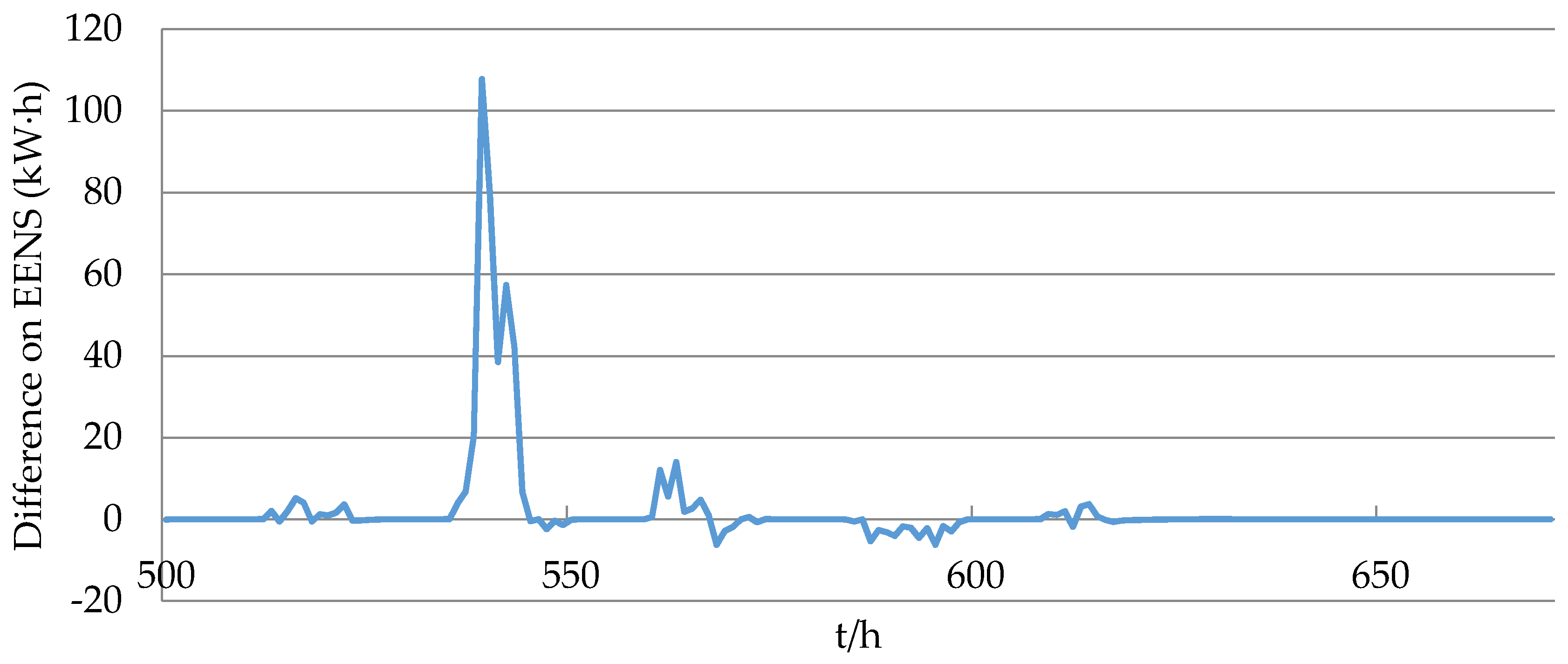
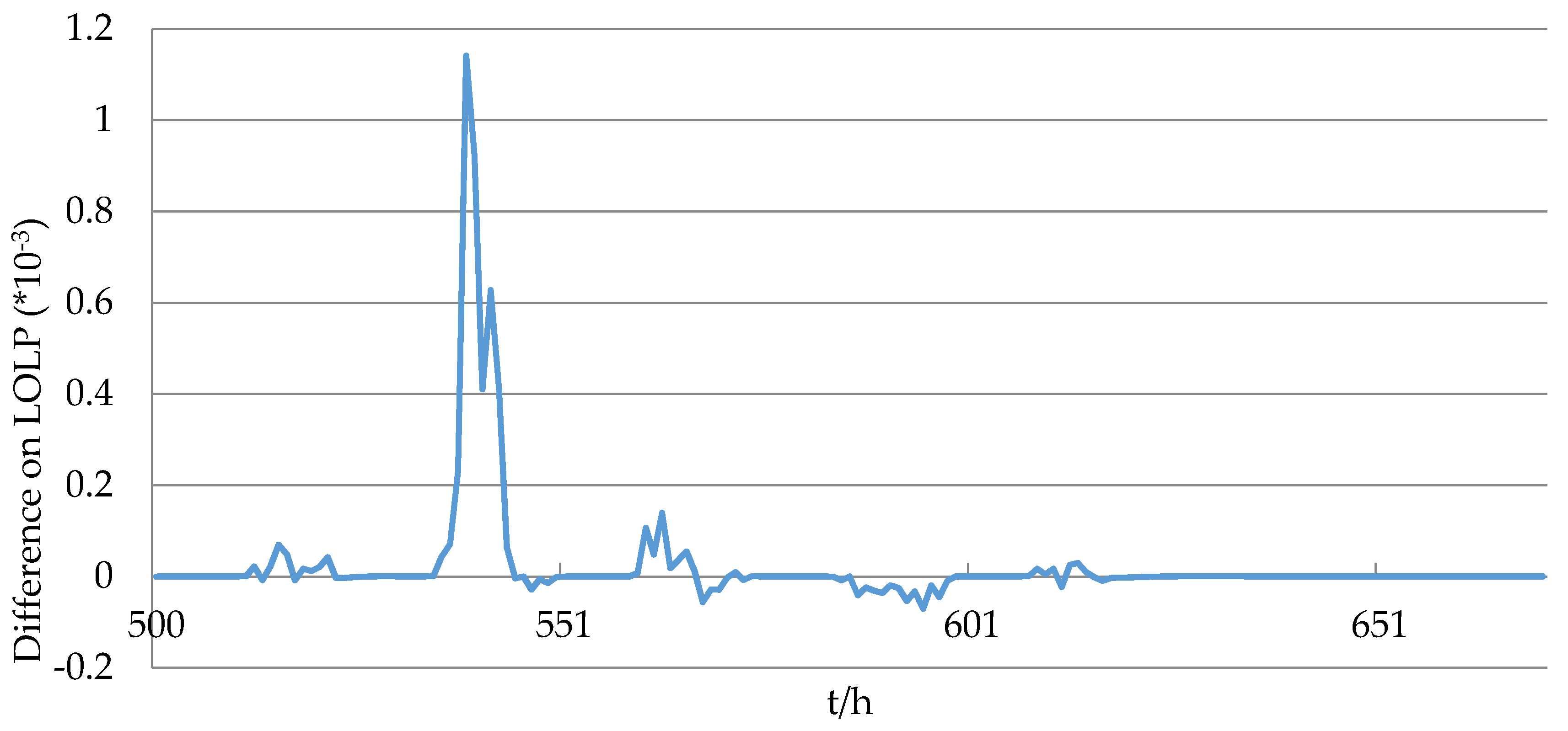
By aid of the introduced UGF algorithm for dependent element and the chronological multi-state wind power model, the proposed UGF based PPS method is applicable for the power system with highly correlated wind power. When compared to the ELDC based approaches, it is more suitable for computer programming when addressing large-scale power system stochastic simulation. While conventional PPS approaches only provide reliability indices for whole simulation period, such as the expected production energy of each generator, expected energy not supplied (EENS), and loss of load probability (LOLP), UGF based probabilistic production simulation could also provide these indices at each moment.

The remainder of the paper is arranged as follows. Chronological multi-state wind power model considering the correlation between wind farms is developed in Section 2. The UGF based PPS considering correlated wind power is introduced in Section 3. Section 4 presents case studies, followed by the conclusion in Section 5.

2. Chronological Wind Power Modelling Considering Correlation

Stochastic time series models of wind speed or wind power built in [17,18,19,20,21] consider both temporal and spatial dependency structures in detail. The data generated by those models restore the correlation between wind farms. But those models could not transform into UGF form. Thus, those approaches cannot be applied to UGF based PPS methods directly. Therefore, the following model is developed.

2.1. Ideology of Chronologically Modeling of Wind Power Considering Correlation

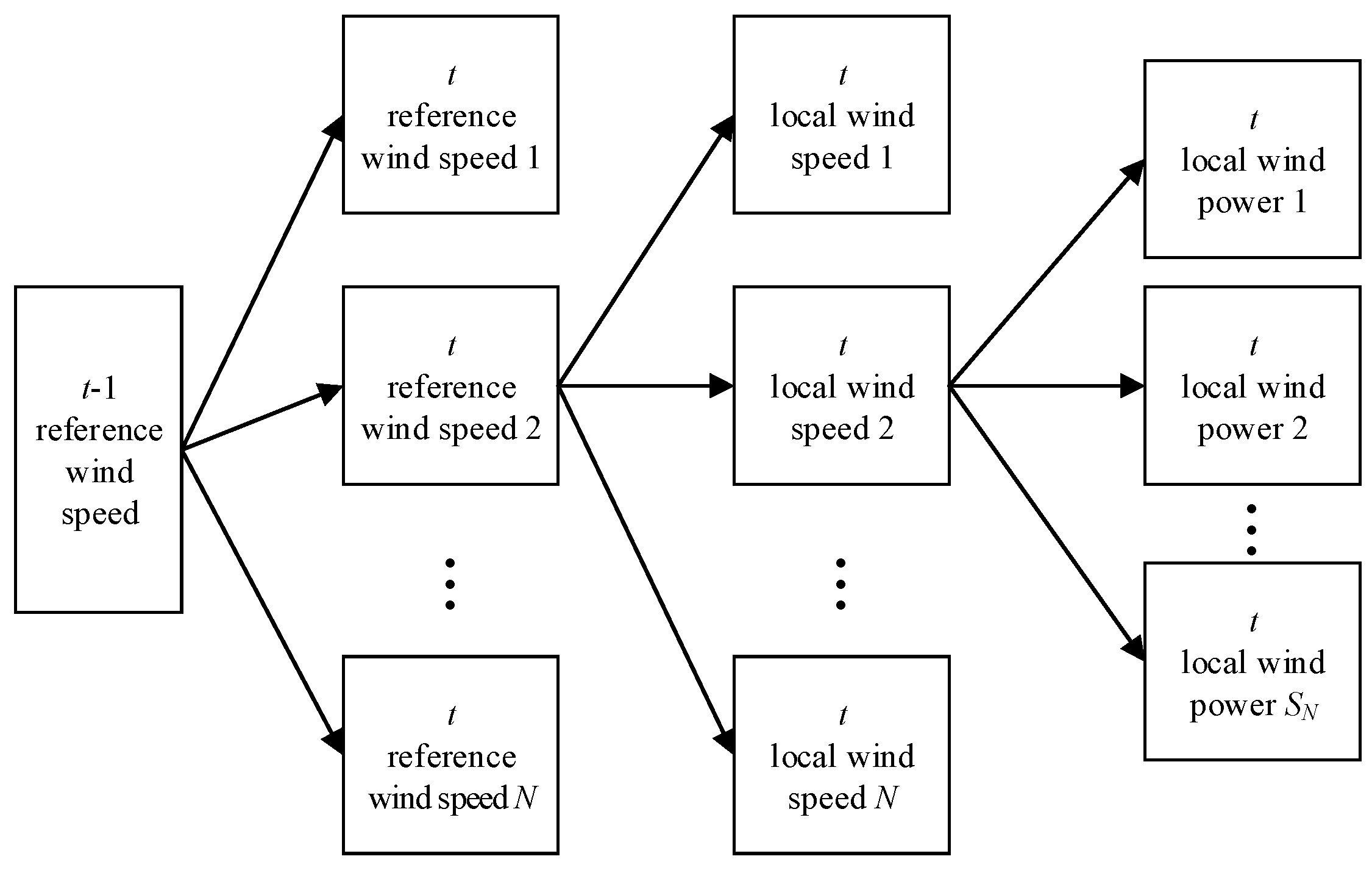
Geographically close wind farms are affected by the same wind source. Therefore their outputs are often highly correlated. But literatures on long-term wind power modeling seldom take both time-varying characteristics and the correlation of wind power into account at the same time. Inspired by the ideology of Markov Process, this paper develops a multi-state wind farm output time series model considering wind speed correlation, which is applicable for the UGF method.

When several wind farms are involved, the following assumptions are posed for simplicity: wind farms could be clustered into several groups; wind farms within one group show an evident correlation, while wind farms from different groups are regarded as independent. Thus, models of wind farms’ output could be developed for each group, and each group’s model has nothing to do with others. In each group, a reference wind farm is chosen out. Other wind farms’ outputs within this group are modelled based on this reference wind speed.

Firstly, a reference wind speed chronological probabilistic model is built by combining the chronologically generated wind speed data and wind speed transition probability of adjacent moments. Secondly, according to the joint distribution of reference wind speed and wind farms’ output, wind power conditional probabilities on different wind speed states are obtained. Finally, wind power chronologically probabilistic models are developed based on the wind speed model and the achieved conditional probabilities.

2.2. Reference Wind Speed Chronologically Probabilistic Model

To ensure an accurate reflection of wind source, the generated reference wind speed should meet three requirements: (a) the probabilistic distribution characteristic of wind speed; (b) diurnal characteristic of wind speed; and, (c) variation characteristic of wind speed. The wind speed generation method in [22] is adopted in this paper. Wind speed simulation data that satisfy unimodal Weibull distribution characteristics of wind speed of the reference wind farm are generated by Probability Measurement Change Method, and the diurnal characteristic is realized by generating daytime and nighttime wind speed, respectively. To satisfy the variation characteristic, the frequency of difference between wind speed values on two adjacent time points is calculated, and based on this statistical frequency, certain simulation data are chosen from the original generated ones as final chronological wind speed data. Detailed procedures refer to [22], not be discussed in detail here.

To reduce the calculation amount, wind speed in a certain interval is taken as one wind speed state and represented by one certain value. For example, wind speed between 0 and 1 m/s is taken as state 1 and represented by 1 m/s when calculating. Chronological wind speed simulation data are generated and are represented as,

$$WS=\{ws(t)\},t=0,1,\dots ,T-1$$

(1)

where ws(t) = 1, 2, …, N, and N is the total number of wind speed states, t is time period, and T is the total number of time period.

Based on historical wind speed data of the reference wind farm, wind speed state transition matrix of adjacent moments is calculated and represented as,

$$P_{tran}=\left[\begin{array}{ccc}{p}_{1,1}& \cdots & p_{1,N}\\ ⋮& \ddots & ⋮\\ p_{N,1}& \cdots & p_{N,N}\end{array}\right]=\left[\begin{array}{c}{p}_1\\ ⋮\\ p_N\end{array}\right]$$

(2)

where p_i,j is the possibility for wind speed transit from state i to state j, and p_i is the ith row of the matrix.

The temporal correlation of wind speed is modelled by those transition probability. If the wind speed state at moment t is ws(t), then at moment t + 1 the probability of each wind speed state wsp(t + 1) is the ws(t)th row of matrix P_tran, namely

$$wsp(t+1)=(p_{ws(t),1},p_{ws(t),2},\dots ,p_{ws(t),N})=p_{ws(t)}$$

(3)

From the above, one can obtain the chronologically probabilistic model of wind speed state as showed in (4). p_ws(t−1),i in this model represents the probability that wind speed is on state i at moment t.

$$WSP=\{wsp(t)\}=\text{{}{p}_{ws(t-1)}\text{}},t=1,2,\dots ,T$$

(4)

2.3. Conditional Probability of Wind Power on Reference Wind Speed

In each group, joint distribution between reference wind speed and wind power’s output is generated by historical data statistics. Then wind power conditional probability of this wind farm under reference wind speed is obtained through joint distribution. The spatial correlation between wind farms is properly modelled in those conditional probability. Referring to the analysis of historical data, wind power is divided into M status by reasonable intervals. The joint distribution is showed in

Table 1. Joint distribution of wind speed states and wind power states.

Wind Speed States	Wind Power States
	1	2	…	M
1	p1,1	p2,1	…	pM,1
2	p1,2	p2,2	…	pM,2
…	…	…	…	…
N	p1,N	p2,N	…	pM,N

where p_i,j is the possibility for wind power state j at wind speed state i.

.

From Table 1, conditional probability of wind power on state j when wind speed is on state i is calculated as follows.

$$p_{j|i}=\frac{p_{j,i}}{{\displaystyle \sum _{k=1}^M{p}_{k,i}}},i=1,2,\dots ,N;j=1,2,\dots ,M$$

(5)

For a group with H dependent wind farms, the conditional probabilities of each wind farm’s output under reference wind speed are obtained by repeating this process, namely $p_{j|i}^1$, $p_{j|i}^2$, …, $p_{j|i}^H$.

2.4. Chronological Multi-State Wind Power Model Considering Correlation

Based on the methods mentioned above, the reference wind speed chronological probability model of reference wind farm and the conditional probability of dependent wind farms is obtained. The probability of reference wind speed on state i at moment t is expressed as p_ws(t−1),i, the probability that wind power of the hth wind farm on state j is $p_{j|i}^h$ when the reference wind speed is on state i. Then, according to the total probability formula, the wind power probability of the hth wind farm on state j at moment t can be expressed as:

$$p_j^h(t)={\displaystyle \sum _{i=1}^N{p}_{ws(t-1),i}\cdot }{p}_{j|i}^h,j=1,2,\dots ,M$$

(6)

Equations (1), (2), (5), and (6) constitute the chronological multi-state wind power models considering correlation, and using these models one can obtain the probability of wind power on a certain state when studying dependent wind farms.

Above all, the logic flow chart of wind power multi-state models can be summarized as Figure 1.

3. Probabilistic Production Simulation Based on Universal Generating Function

Universal generating function is an intuitively simple, efficient expression, and operational tool for discrete random variable, proposed by Professor Ushakov in 1986 [23], and was then applied to reliability assessment of multi-state systems [24,25,26,27]. In the UGF theory, a discrete random variable is expressed in polynomial form, and the polynomial operator is defined according to the operational rule of the variables. The main advantage of UGF is that it offers a systematically recursive computation method for complex composition computation, which is very suitable for computer programming in this regard.

The u-function is the core of the UGF technique. Although it uses a polynomial form, the u-function is essentially different from the polynomial: (a) the coefficients and indices of variables in the u-function are not necessarily scalar, but also other math objects; (b) operator of the u-function is different from the polynomial operator, and its specific calculation requires further analysis. But the UGF operator holds the nature of recursive. Thus, a good adaptability for large-scale computer arithmetic is guaranteed.

3.1. Modeling Conventional Generation Unit’s Output

In the UGF based PPS method, the stochastic characteristics of power sources in the system are modelled by UGF in multi-state elements, then the whole system is seen as an equivalent multiple state system. The output of generation source is regarded as a discrete random variable with a certain p.m.f. The model of equivalent generation source is obtained by modeling each generation source and integrating these models into one. Then, this model is used to match with the load on each moment to realize the supply and demand balance during a certain simulation period [12].

Suppose that conventional generation units in a power system are put into operation in a planned order (which is generally determined by the unit’s economic or environmental characteristics), and at moment t, N independent conventional units have been put into operation. When considering the random failure of units, the UGF model of the nth unit at moment t is,

$$u_n(z,t)={\displaystyle \sum _{i_n=1}^{S_n}{p}_{i_n}^n(t)\cdot z^{P_{t_n}^n(t)}},n=1,2,\dots ,N$$

(7)

where S_n is the total number of the nth unit’s state; $P_{i_n}^n$(t) is the output of the nth unit on state i_n at moment t; $p_{i_n}^n$(t) is the corresponding probability.

Then the UGF model of the equivalent multi-state system comprising of N units is as follows,

$$u_{S_N}(z,t)=\otimes (u_1(z,t),u_2(z,t),\cdots ,u_N(z,t))={\displaystyle \sum _{j_{S_N}=1}^{S_{S_N}}{p}_{j_{S_N}}^{S_N}(t)\cdot z^{P_{j_{S_N}}^{S_N}(t)}}$$

(8)

where $S_{S_N}$ is total number of the equivalent system’s state after N units put into operation; $P_{j_{S_N}}^{S_N}$(t) is the output of the equivalent system on state $j_{S_N}$ at moment t; $p_{j_{S_N}}^{S_N}$(t) is the corresponding probability.

3.2. Modeling Wind Farm Outputs Considering Correlation

The models mentioned above are based on the premise that each generator is independent of each other. In this section, UGF algorithm for dependent random variables is adopted [24,25]. Wind farms are divided into groups, and the UGF model of each group is developed while considering correlation. Eventually, each group is equivalent to one generation unit.

Supposing that wind farm A, B, and C show an evident correlation, but are independent from other wind farms. They could be clustered into one group to develop a UGF model. Choose A as the reference wind farm and its wind speed as the conditional random variable, and use the method in Section 2.4 to obtain the conditional probabilities of these three wind farms’ outputs regarding to wind speed of wind farm A. the UGF models are developed as follows.

The UGF model of wind farm A’s output at moment t is:

$$\begin{array}{l}{\overline{u}}_A(z,t)={\displaystyle \sum _{i=1}^{S_A}{\overline{p}}_i^A(t)z^{P_i^A(t)}}\\ {\overline{p}}_i^A(t)=(p_{i|1}^A(t),p_{i|2}^A(t),\dots ,p_{i|N}^A(t))\end{array}$$

(9)

where $P_i^A$(t) is the output of wind farm A on state i; ${\overline{p}}_i^A(t)$ is the conditional probability vector of $P_i^A$(t), and $p_{i|s}^A$(t) is the corresponding conditional probability under the condition that wind speed is on state s; N is the total number of the wind speed state; S_A is the total number of wind farm A’s output state.

Similarly, UGF models of wind farm B and C, respectively, at moment t are:

$$\begin{array}{l}{\overline{u}}_B(z,t)={\displaystyle \sum _{j=1}^{S_B}{\overline{p}}_j^B(t)z^{P_j^B(t)}}\\ {\overline{p}}_j^B(t)=(p_{j|1}^B(t),p_{j|2}^B(t),\dots ,p_{j|N}^B(t))\end{array}$$

(10)

$$\begin{array}{l}{\overline{u}}_C(z,t)={\displaystyle \sum _{k=1}^{S_C}{\overline{p}}_k^C(t)z^{P_k^C(t)}}\\ {\overline{p}}_k^C(t)=(p_{k|1}^C(t),p_{k|2}^C(t),\dots ,p_{k|N}^C(t))\end{array}$$

(11)

The outputs of those three wind farm are all related to wind speed A. According to the UGF computing approach for dependent random variables, the UGF models of these three wind farms are integrated and computed as follows (the variable t is omitted for simplicity).

$$\begin{array}{c}{\overline{u}}_{eq}(z)=\otimes ({\overline{u}}_A(z),{\overline{u}}_B(z),{\overline{u}}_C(z))={\displaystyle \sum _{i=1}^{S_A}{\overline{p}}_i^A{z}^{P_i^A}}\otimes {\displaystyle \sum _{j=1}^{S_B}{\overline{p}}_j^B{z}^{P_j^B}}\otimes {\displaystyle \sum _{k=1}^{S_C}{\overline{p}}_k^C{z}^{P_k^C}}\\ ={\displaystyle \sum _{i=1}^{S_A}{\displaystyle \sum _{j=1}^{S_B}{\displaystyle \sum _{k=1}^{S_C}{\overline{p}}_i^A\circ {\overline{p}}_j^B\circ {\overline{p}}_k^C{z}^{P_i^A+P_j^B+P_k^C}}}}\end{array}$$

(12)

where

$${\overline{p}}_i^A\circ {\overline{p}}_j^B\circ {\overline{p}}_k^C=(p_{i|1}^A\cdot p_{j|1}^B\cdot p_{k|1}^C,p_{i|2}^A\cdot p_{j|2}^B\cdot p_{k|2}^C,\dots ,p_{i|N}^A\cdot p_{j|N}^B\cdot p_{k|N}^C)$$

(13)

The final computation result, conditional probability model of equivalent wind farm, is expressed in (14). This model means that A, B, and C are equivalent to one wind farm containing S_eq output states, and under the condition that wind speed A is on its state n, the conditional probability of this unit on its state m is $p_{m|n}^{eq}$.

$${\overline{u}}_{eq}(z)={\displaystyle \sum _{m=1}^{S_{eq}}{\overline{p}}_m^{eq}}{z}^{P_m^{eq}},{\overline{p}}_m^{eq}=(p_{m|1}^{eq},p_{m|2}^{eq},\dots ,p_{m|N}^{eq})$$

(14)

According to the model in Section 2, wind speed probabilistic time series of wind farm A is generated and expressed as (4), then the UGF model of wind speed A at moment t is as follows.

$$u_{WS}(z,t)={\displaystyle \sum _{s=1}^N{p}_{ws(t-1),s}{z}^s}$$

(15)

The equivalent UGF model of these three wind farms is,

$$U(z)=\otimes (u_{WS}(z),{\overline{u}}_{eq}(z))={\displaystyle \sum _{s=1}^N{p}_{ws(t-1),s}{\displaystyle \sum _{m=1}^{S_{eq}}{p}_{m|s}^{eq}{z}^{P_m^{eq}}}}={\displaystyle \sum _{m=1}^{S_{eq}}\left({\displaystyle \sum _{s=1}^N{p}_{ws\left(t-1\right),s}\cdot }{p}_{m|s}^{eq}\right)z^{P_m^{eq}}}$$

(16)

For other groups, their equivalent UGF models are developed by repeating this progress. In this way, all of the wind farms in the system are equalized into several independent units. Their UGF models are developed. Along with the conventional units’ models, these models could be utilized to conduct PPS based on the UGF operation.

3.3. UGF Based PPS Approach

Load of the system at moment t is expressed as L(t). To supply this load, generation units are put into operation in planned order (for example in the order of descending incremental production cost), and the arrangement is done until the capacity of the equivalent unit for N units put into operation is equal or greater than L(t), or all of the units have been put into operation. After N units have been scheduled, the loss of load probability (LOLP), expected energy not supplied (EENS) of the system, and the expected power generation of each unit could be calculated as follows.

Supposing that the system outputs on different states are $P_1^{S_N}$, $P_2^{S_N}$, …, $P_{S_N}^{S_N}$ (sorted in an ascending order), and the corresponding probability is $P_1^{S_N}$, $P_2^{S_N}$, …, $P_{S_N}^{S_N}$. If there is a number d that satisfies $P_d^{S_N}<L\left(t\right)<P_{d+1}^{S_N}$, then the index LOLP of the system with N units on operation at moment t is equal to the sum of the probabilities of which the system output is less than L(t), namely

$$LOL{P}_N(t)={\displaystyle \sum _{j_{S_N}=1}^d{p}_{j_{S_N}}^{S_N}(t)}$$

(17)

When the system generation output is less than L(t), the energy not supplied can be obtained by multiplying the difference between the output and L(t) with the time interval (one hour in this paper). Multiply this energy with the corresponding probability, and sum up all of the results, then the index EENS of the system with N units on operation at moment t is obtained, namely

$$EEN{S}_N(t)={\displaystyle \sum _{j_{S_N}=1}^d[L(t)-P_{j_{S_N}}^{S_N}(t)]\cdot 1\cdot p_{j_{S_N}}^{S_N}}$$

(18)

The expected generated energy of the Nth unit at moment t is the difference of EENS when N − 1 units and N units are put into operation, namely

$$E_N(t)=EEN{S}_{N-1}(t)-EEN{S}_N(t)$$

(19)

For every moment in simulation period, units could be put into operation by certain order and use the proposed approach above to calculate these three indices. After the simulation for each period, the total power generation of each unit, and LOLP, EENS of the whole system during the whole simulation period could be worked out. Taking two indices: LOLP(t) and EENS(t) as example after all units have been arranged, the index LOLP during the whole period is calculated like,

$$LOLP=\frac{1}{T}{\displaystyle \sum _{t=1}^{T}LOLP(t)}$$

(20)

The index EENS during the whole period is calculated like,

$$EENS={\displaystyle \sum _{t=1}^{T}EENS(t)}$$

(21)

The expected generation of each unit during the whole period is calculated as follows,

$$E_N={\displaystyle \sum _{t=1}^T{E}_N(t)}$$

(22)

Here T refers to the simulation period. The flowchart of this approach is shown in Figure 2.

4. Case Studies

Four cases are implemented and discussed in this part. Case one is used to verify the correctness of the adopted correlation model. The other three cases are based on the modified IEEE-RTS 79 system. The second one includes no wind farm, aiming to verify the proposed approach by comparing it with conventional approaches. The third one with two dependent wind farms is used to analyze the impact whether considering their correlation or not on simulation results. The fourth one, also with two wind farms but with a variety of correlation characteristics, is used to analyze the influence of different correlations on the results. The former three cases demonstrate the correctness of the proposed method. The third and fourth cases demonstrate the necessity of correlation modeling. The original data can be referred to [28]. Conventional units are arranged by the order of descending full load average cost (that is the unit’s average cost at its maximum output), and wind power has the highest priority.

4.1. Verification of the Correctness of the Proposed Approach

Wind speed generation method in [22] guarantees the simulation data of wind speed in accordance with the historical characteristics. Thus, the first case mainly tests the proposed wind speed correlation modeling method. Some adjustments are made to make the results more intuitive. Since wind farm’s power output can be obtained easily from its wind speed, so this case only focuses on the comparison of the generated wind speeds considering the correlation with the historical wind speeds. This case reproduces the first two steps of Figure 1, the multi-state model of wind speed is obtained. Then, the simulation data were generated by the Monte Carlo method. Five years of historical data of a certain month of highly correlated wind farm A and B is taken as raw data. Select wind speed of wind farm A as the reference one, and then wind speed of wind farm B is generated through reference wind speed A by the proposed method. The comparison of historical and generated wind speed of wind farm B is done on the Weibull parameters, spatial correlation coefficient with wind farm A and autocorrelation function at lag 1, the results are shown in

Table 2. Comparison on generated wind speed simulation data.

Data	Weibull Scale Parameters	Weibull Shape Parameters	Spatial Correlation Coefficient with A	Autocorrelation Function at Lag 1
Historical Data	9.361	1.574	0.673	0.845
This paper	9.322	1.596	0.668	0.732

.

The Weibull parameters of generated data are basically consistent with the historical data. The spatial correlation coefficient between generated data and the reference wind speed (wind speed of A) is close to the spatial correlation coefficient between historical data and the reference wind speed (the difference is less than 1%). The autocorrelation function at lag 1 of generated data is also close to historical one. This shows the validity of the proposed correlation modeling algorithm. When compared with other correlation modelling approaches, the correlation model proposed in this paper is simple but with high accuracy, and it is applicable for the UGF based PPS approach.

Based on the IEEE-RTS79 system, the proposed approach is used to conduct the simulation. The simulation period is 8760 h with 1 h resolution. The comparison among the results given by the proposed approach in this paper, precise results by analytical method in [29], and the results obtained by the serialized PPS approach in [11] is shown in

Table 3. Comparison on simulation results without wind farms.

Indices	Ref. [29]	Ref. [11]	This Paper
EENS (GWh)	1.176	1.175	1.176
LOLE (hour/year)	9.394	9.367	9.394
Total Supplied Energy (GWh)	15,295.898	15,295.867	15,295.898

.

As is shown in Table 3, as for the indices EENS, LOLP, and total energy generation, the proposed approach is as accurate as that in [29], and more accurate than serialized PPS approach. This result verifies the correctness and the effectiveness of the proposed approach. In comparison to the serialized PPS approach [11], the proposed approach is advantageous on its brief expression, recursive operation in nature, which is more suitable for computer arithmetic. Thus, a more precise result is obtained.

4.2. Influence of Correlation Degree on the Results

Two wind farms are added to the IEEE-RTS79 system, whose capacities are 200 MW and 100 MW, respectively. The scale parameter and shape parameter of wind speed Weibull distribution for 200 MW wind farm are 13.3694 and 1.9945, respectively, and those of 100 MW wind farm are 7.7439 and 1.5823, respectively. The correlation coefficient is assumed to be 0.7081. The simulation period lasts from the 19th week to the 22nd week. The proposed approach is applied to conduct the simulations for two scenarios. One is considering the correlation between two wind farms; the other one is ignoring the correlation between these two wind farms. Two systems without wind farm and with equal additional conventional units are taken as the reference ones. The simulation results are shown in

Table 4. Comparison on simulation results containing wind farms.

Indices	w/o Wind Farm	Considering Correlation	Not Considering Correlation	with Additional Conventional Units
EENS (MWh)	62.737	23.082	21.481	3.682
LOLP (×10−4)	8.43	3.25	3.06	0.622
Wind Power Supplied Energy (GWh)	0	103.374	100.998	0
Standard Deviation	-	49.9	48.4	-

.

When compared to the scenario without wind farm, EENS and LOLP drop evidently when two wind farms are integrated in, which implies that two wind farms integration improves the system reliability. But, those indices are not as good as the system with equivalent conventional capacity. This is because an extra power source of 300 MW is integrated in the system, leading to a rise in generation capacity while the load remains unchanged. Naturally, the system becomes more reliable. Due to the reliability of wind power is worse than conventional units, reliability indices of the system with equal conventional capacity are better than the system with wind power.

If the correlation of two dependent wind farms is neglected, wind power supplied energy is almost the same when compared to the scenario when correlation is considered (only 2% less), but EENS and LOLP of the whole simulation period are evidently reduced. For further analysis, the differences in EENS and LOLP (between the results with and without the correlation into account) in each simulation period are computed. They are partly illustrated in Figure 3 and Figure 4, respectively. As is shown in the figures, when the load is low and the generation capacity is rather abundant, the differences are quite small, that means whether considering the correlation or not does not exert an apparent influence on the system reliability; however, when the load is high and the generation capacity is relatively short, EENS and LOLP become smaller if the correlation is not considered. This fact implies that the reliability analysis result might be too optimistic if the correlation is not considered.

Since two wind farms show a strong correlation (the correlation coefficient is 0.7081, near to 1), which means similar variations of two wind farms’ output, consequently the variations enhance each other, making the variation of total wind power output quite intensive. When correlation is not considered, this effect is not accurately reflected, making the reliability indices more optimistic than the actual situation. The last line of Table 3 is the standard deviation of wind power time series under the two different situations. The standard deviation is reduced when neglecting correlation, implying a relatively stationary wind power process.

To study the influence of different correlation degrees on the PPS results, two dependent wind farms are added to the IEEE-RTS79 system. The capacities are still 200 MW and 100 MW, respectively, with five correlation degrees of 0.7081, 0.4115, 0.0084, −0.3501, and −0.6507, respectively. The simulation period lasts from the 19th week to the 22nd week and the results are shown in

Table 5. Comparison on the results of the five cases.

Indices	Correlation Coefficient
	0.7081	0.4115	0.0084	−0.3501	−0.6507
EENS (MWh)	23.082	22.429	20.508	19.288	18.286
LOLP (×10−4)	3.25	3.18	2.94	2.78	2.64
Wind Power Supplied Energy (GWh)	103.375	104.132	101.922	102.355	103.757

.

These five scenarios represent five correlation situations: evidently positive correlation, positive correlation, uncorrelated, negative correlation, and evidently negative correlation. Wind power supplied energy of these cases are almost the same, with a difference of 2.16% between the maximum and the minimum. This shows that the correlation degree would not lead to an observable impact on wind power supplied energy. The reliability indices EENS and LOLP present a downward trend as the correlation varies from evidently positive to evidently negative. Meanwhile, from the standard deviation’s variation tendency given in Figure 5, it can be observed that wind power time series fluctuation is also becoming weaker. The analysis above implies that the correlation degree of wind power series would impact the reliability indices a lot: negatively correlated wind power leads to optimistic reliability indices, and the smaller the correlation coefficient, the more optimistic the indices would be, if correlation is not taken into account.

5. Conclusions

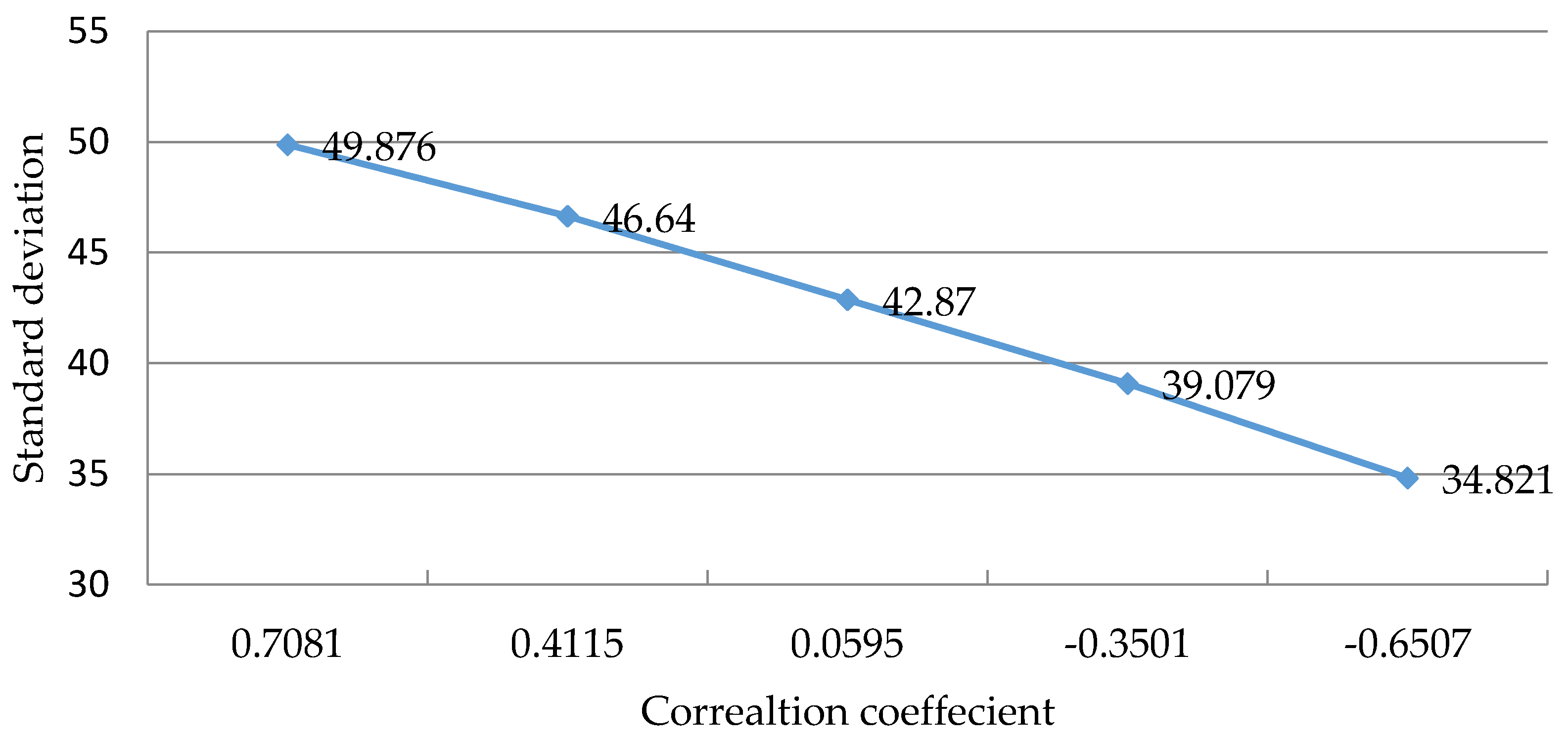
For the issue of stochastic production simulation of the system with high share of wind power, this paper proposed a universal generating function based probabilistic production simulation approach considering the spatial-temporal correlation simultaneously. (1) Wind speed is modeled by probability measurement change method, the temporal correlation between the same wind power series and the spatial correlation between the different wind power series are well described; (2) the technique that wind farms are clustered into different groups independent of each other by correlation is efficient in computation. The correlation is formulated as the conditional probability of each wind power under the reference wind speed, which is easy to integrate into the UGF operation; (3) by aid of the introduced UGF algorithm for dependent element, the proposed UGF based PPS is applicable for the power system with highly correlated wind power; (4) EENS, LOLP, unit supplied energy at each moment as well as the whole simulation period is calculated.

When compared to the traditional PPS methods, the proposed model takes both time-varying information of the system and wind power correlation into consideration. Unlike conventional ELDC based methods, a more accurate and detailed results in the aspects of production cost and reliability indices are provided by the proposed approach. When compared to the methods that are considering time-varying information, like the SOT approach, not only wind power correlation is addressed, but also the UGF operation shows a better adaptability for large scale systems than the conventional convolution operation.

As a whole, the proposed approach could be a useful tool for power generation planning, real-time electric power and electric energy balance analysis, and online reliability evaluation.