
Energy and Reserve under Distributed Energy Resources Management—Day-Ahead, Hour-Ahead and Real-Time


1
INESC Technology and Science (INESC TEC), 4200-465 Porto, Portugal
2
Department of Electrical Engineering, Research Group on Intelligent Engineering and Computing for Advanced Innovation and Development (GECAD), Institute of Engineering-Polytechnic of Porto (ISEP/IPP), 4249-015 Porto, Portugal
3
Department of Electrical Engineering, Technical University of Denmark, 2800 Kongens Lyngby, Denmark
*
Author to whom correspondence should be addressed.
Energies 2017, 10(11), 1778; https://doi.org/10.3390/en10111778
Submission received: 25 September 2017
/
Revised: 17 October 2017
/
Accepted: 27 October 2017
/
Published: 4 November 2017
(This article belongs to the Section F: Electrical Engineering)
Abstract
:The increasing penetration of distributed energy resources based on renewable energy sources in distribution systems leads to a more complex management of power systems. Consequently, ancillary services become even more important to maintain the system security and reliability. This paper proposes and evaluates a generic model for day-ahead, intraday (hour-ahead) and real-time scheduling, considering the joint optimization of energy and reserve in the scope of the virtual power player concept. The model aims to minimize the operation costs in the point of view of one aggregator agent taking into account the balance of the distribution system. For each scheduling stage, previous scheduling results and updated forecasts are considered. An illustrative test case of a distribution network with 33 buses, considering a large penetration of distribution energy resources allows demonstrating the benefits of the proposed model.
1. Introduction
1.1. Background, Methodology and Aim
The increasing penetration of distributed energy resources (DERs), including distributed generation (DG), demand response (DR), energy storage systems (ESSs) and electric vehicles (EVs) leads to the need to develop new intelligent and hierarchical methods for power systems operation management [1]. As these resources are mostly connected to the distribution network, it is important to consider the introduction of these types of resources in the ancillary services (AS) delivery in order to achieve greater reliability and cost efficiency of power systems operation [2,3].
In this new paradigm of power systems operation, the independent system operator will consider the existence of virtual power players (VPPs) with capability to aggregate all type of small scale DERs, which are unable to individually engage themselves in the electricity market [4,5]. This implies that the AS procurement by the VPP is targeted to the distribution network [6]. Thus, VPP should consider the establishment of complex offers with the DERs in order to ensure reserves levels and quality of AS that suits the needs of the distribution network. In this context, the operation and control of future distribution network and smart grid are expected to engage in the following AS, provided by the distribution system operator or by the VPP [7]: frequency regulation; voltage regulation; congestion management; optimization of grid losses and fault-ride-through capability service. However, a better coordination between the transmission and distribution system operators is necessary to provide AS in the future power systems, namely at frequency regulation [8].
The role of VPPs, and other aggregator players in general, is not yet well established and the electricity markets are not adapted to this new reality [9]. In most of the present electricity markets, DERs cannot participate in AS. However, this reality will probably be different in a near future due to the high incentives to increase the use of renewable resources. This means that VPPs should manage their resources not only to participate in traditional services (sell energy) but also in other type of services.
Within this scope, this paper proposes a tool to joint schedule energy and reserve in a distribution network level considering the ability of the virtual power player to aggregate and manage DERs. The model considers primary frequency reserve, i.e., reserve down (RD) and reserve up (RU). Three different levels of RU are modeled to be used by this tool, considering different response times and prices. Other important aspect of the proposed tool is the joint optimization of energy and reserve in different time-horizons (day-ahead, hour-ahead and real-time), considering the different characteristics in each one. This tool is relevant in players managing local energy systems, such as part of distribution grid, micro-grid and community system. For instance, this tool can be used by a VPP that manages DERs and grid after substation to determine the amount of energy and reserve in case the whole energy system cannot support his reserve service.
1.2. Literature Review and Specific Contributions
For optimal integration of DERs in energy and ancillary services, new business models and scheduling processes should be thought of. The literature on the management of DERs considering day-ahead, hour-ahead and real-time scheduling processes has been growing over the last few years [5]. This includes a number of studies on day-ahead scheduling for DERs with impact on operation costs [10,11,12,13], optimal bidding [13], load shedding [10], carbon emissions [10,14], EVs with vehicle-to-grid ability [15,16], losses reduction [17] and service restoration [18], as well as ancillary services management [19,20], among others. An integrated day-ahead and hour-ahead (intraday) schedule for dealing with DERs uncertainty [21], maximizing the retailer’s profit under carbon emissions penalties [22], DERs scheduling with recourse to stochastic programming [23] and control strategies [24] has been studied. In [25], a simulator for hour-ahead and real-time scheduling of DERs is proposed, considering the minimization of operation costs. Furthermore, real-time adjustments of DERs taking into account the operation costs [26,27], DERs profit [28], ancillary services [19,29,30,31] and control strategies [24] are crucial to maintain the system balance. Integrated tools for simulation of DERs energy scheduling under day, hour-ahead and real-time has been developed, minimizing the operation costs [32]. Nevertheless, [33,34] proposed a day-ahead joint scheduling of energy and reserve taking into account the uncertain production of DERs under distribution systems and micro-grid management, respectively.
In general, the literature has paid little attention to the joint scheduling of energy and reserve for DERs, considering the different time-horizons. Such DERs joint optimization on day, hour-ahead and real-time is expected to bring additional revenues to DERs as well as to improve system stability, safety, quality, reliability and competitiveness of demand and supply.
In this context, a tool is developed to support the joint optimization of energy and reserve with large-scale penetration of DERs. Additional input variables include forecast of generation and demand resources for each time-horizons of simulation. The tool is applied and demonstrated on a 33-bus distribution network with high penetration of DERs (mainly, wind, photovoltaic, combined heat and power (CHP), fuel cell, biomass, small hydro, waste-to-energy units, ESSs, EVs with vehicle-to-grid ability, curtailment and reduce DR programs, and upstream providers).
1.3. Paper Organisation
The rest of this paper is organized as follows. Section 2 states the assumptions and features of the proposed model to manage energy and reserve at distribution level for different scheduling periods. Section 3 describes the mathematical details of the model for each scheduling period. Section 4 test and validate the operation of the model through a detailed case study. Section 5 assembles the most important conclusions and discussion.
2. Model Features
A methodology for the joint scheduling of the energy and reserve at distribution network level is proposed. The methodology includes different AS, such as RD and three levels of RU (RU_1. RU_2 and RU_3). Different response times and prices are associated to these three upward reserve levels. Thus, there is a hierarchy of deployment, where the RU_1 is the first service to be deployed and RU_3 the last one to be deployed. The model allows trading between DERs and VPPs based on special contracts, which may be favourable for small DERs that can participate in the schedule through the aggregation of a VPP, and therefore be beneficial for the VPP to ensure greater flexibility in its optimal management. The proposed model consists in three main stages represented in Figure 1. Each stage corresponds to a different time-horizon scheduling (day-ahead, intraday or hour-ahead, and real-time).
2.1. First Stage—Day-Ahead Scheduling
A day-ahead optimization model for the 24 h of the next day with the objective of minimizing the VPP operation costs for energy and reserve is proposed. Additionally, the forecast for DERs and reserve requirements needed to ensure the proper operation of power systems are considered.
2.2. Second Stage—Intraday Scheduling
An hourly schedule of resources for the overall period of 24 h based on the scheduling obtained in the first stage is performed. Furthermore, the model considers a more accurate forecast of the demand and generation availability, which is important when considering the generation of renewable sources and their uncertainty. At this point, the RD and RU requirements are updated, rescheduled and suited according to the system needs.
The use of an hourly forecast for consumption and generation is important for the proper optimization of the intraday scheduling. Thus, the developed tool becomes more comprehensive and easy for real applications. The intraday (hour-ahead) optimization process considers not only the forecast for demand and generation, but also the energy scheduled in the resources in the first stage (i.e., day-ahead scheduling). Thus, the minimum and maximum limits of generation resources for each hour are used according to the situation of energy balance constraint, i.e., when there is surplus of generated energy (overproduction) or when there is shortage of generated energy (overconsumption) in the energy balance constraint after the forecast, the generation limits for each resource are suitable to each simulation.
2.3. Third Stage—Real-Time Scheduling
An optimization every 5 min over a total period of 24 h based on the scheduling obtained in the second stage and on the real demand and generation is performed. In addition, the reserve that was scheduled in the second stage (intraday) is partially or totally used as energy to ensure the proper operation and reliability of the power system.
3. Model Formulation
This section provides the formulation of the optimization problem for each of the model stages.
3.1. Day-Ahead Model
The objective function has the main goal of minimizing the VPP operation costs including the energy and all AS (k) during the period T.
where represents the function for optimizing all resources that may participate in energy commodity, determined as
where the index k equal 5 corresponds to the energy service. , is the cost with external suppliers, is the cost with DG units, is the cost with storage discharge, is the cost with storage charge, is the cost with EV discharge, is the cost with EV charge, and are the cost with DR program for reduction and curtailment, respectively. is the cost with non-supplied demand and is the cost with generation curtailment power for DG units.
The function of AS costs is given by
where, the index k represents the four reserve services that go from 1 to 4 representing RD, RU_1, RU_2 and RU_3, respectively. and are relaxation variables that are activated to meet the difference between the service requirement and the power supported by market participants, if all participants in each service cannot satisfy the requirement of each service. Then, the VPP procures resources able of satisfying the variable through bilateral contracts. These variables allow the reserve dispatch to be feasible if market participants fail to meet the reserve requirements.
The active power balance in bus i for period t is defined as
such that is the total active power generation and is the total active power demand, while is the load demand. The reactive power balance in each bus i for each period t is given by
where is the total reactive power generation and is the total reactive power consumption. The bus voltage magnitude and angle limits are represented in (6) and (7). To the slack bus, the voltage angle and magnitude are fixed and defined by the VPP.
The power flow from bus i to bus j (8) and from bus j to bus i (9) must be lower than the line thermal limit, and is given by
such that is the voltage in polar form, is admittance of line and is the maximum apparent power (or thermal limit) in the line.
The minimum and maximum amount of active power generation provided by external suppliers (10) and DG units (11) for energy and reserve services is defined as
where is a binary variable of DG units.
For DG units with “take-or-pay” contracts established with VPP, mainly generators based on renewable sources, the following constraint is applied:
The sum of the active power generation from energy, RU_1, RU_2 and RU_3 services must be lower or equal then the power capacity of external suppliers (13) and DG (14), as given by
where, the index ke corresponds to the energy service.
The difference between the active power generation from energy and RD services must be higher or equal to a minimum power limit for external suppliers (15) and DG units (16), as
The reactive power generation limits for external suppliers (17) and DG units (18) are given by
The upper limits for DR programs of reduction and curtailment in day-ahead are defined by
The storage technical limits in each period t combine several distinct constraints (21) to (31). In each period t should be ensured non-simultaneity (21) of the storage charge and discharge ability for the energy and AS services, where there is binary variables for storage discharge and storage charge . The charge limit for each storage unit considering the battery charge rate is in (22). The storage discharge limit (23) based on the battery discharge rate is considered.
The maximum battery charge limit for upward reserve services (24) is related to the flexibility of the storage in the upward reserve services, in which the charge acquired in energy commodity can be reduced. The maximum battery discharge limit for upward reserve services is in (25). The battery balance at each period t needs to be between a lower and upper limit (26). The battery balance (27) for upward reserve services considering the remaining energy from precious period and the charge and discharge ability are performed, where is the energy stored for upward reserve services and the yield of charge and discharge process of the electricity network to the storage unit.
The technical constraints are defined as
The maximum charge and discharge limit of battery for energy and downward reserve services is detailed in Equations (28) and (29), respectively. The battery power balance for energy and downward reserve services is between a lower and upper limit (30). The battery power balance for energy and downward reserve services is determined in (31).
The model enables the integration of EV resources in the energy management, safeguarding each individual vehicle characteristics and needs. The non-simultaneity of the EV charge and discharge is in (32). The charge (33) and discharge (34) limit for EVs are also considered in this model. The minimum and maximum stored energy in the EV is in (35). The maximum limit corresponds to the battery’s capacity. On the other hand, the minimum limit will be informed by the EV user to the VPP that corresponds to the minimum amount of energy to guarantee at the end of that period. The energy balance of the battery is in (36), where is the energy consumption during a trip of the EV. This energy consumption can be sent by EV owner [35] or a forecast tool can be used [36] to predict EVs owners behavior.
The downward reserve service requirement can be provided by external suppliers, DG and ESS units, and is defined as
where is the reserve service requirement. The limits for the reserve requirements are constrained by
3.2. Intraday Model
The formulation of the intraday (hour-ahead) model is based on the first stage. The optimization process is performed every hour based on the new generation and demand forecast. During the optimization process is analysed the power imbalance on the system, where the resource limits are updated taking into account the sign of system imbalance (overproduction or underproduction) Figure 2.
In case of excess of generation (overproduction), the resources limits can be between the minimum and the scheduled value in first stage (day-ahead scheduling) obtained for the generation resources. On the other hand, when there is lack of generation, the generation resource limits are between the value obtained in the first stage and its maximum available power.
3.3. Real-Time Model
The real-time optimization is performed every five minutes for the entire time-horizon, considering the intraday scheduling and the forecast every 5 min. The optimization process analyzes the system imbalance where previous scheduled AS are used to balance the system. Thus, the real-time simulation model is slightly different from the model used in the first and second stage. Most of the equations remain the same, but with the introduction of different time dimension. The formulation is adapted to consider a simulation every five minutes in each hour, where the objective function is defined as
In this model, ancillary services are applied taking into account its hierarchy and the system imbalance. Thus, some constraints are added to the model depending on the system imbalance. In case of overproduction, downward reserve services are activated and DG variables are redefined as
where is the final energy scheduled in the simulation and used in the power flow, while is a binary variable to activate downward reserve service. This principle is applied for the remaining type of resources. On the other hand, when there is underproduction, upward reserve services are activated and DG resources are modeled as
where is the binary variable to activate upward reserve services. Following the same concept, DR resources are available to provide upward reserve services by decreasing the consumption.
Non-simultaneity between the activation of upward and downward reserve services is assumed as
4. Case Study
In this section, a case study is used to illustrate the main features of the proposed model and its consistent behaviour. Furthermore, this case study shows the appropriate performance and the practical relevance of the proposed model. The effectiveness of this model is validated comparing the outcomes of each stage of the model. The mixed integer nonlinear programming (MINLP) model described in the previous section is solved using the discrete and continuous optimizer (DICOPT) [37] under the general algebraic modeling system (GAMS) [38] on an Intel Zeon W5450 processor, with eight cores clocking at 3.0 GHz and 12 GB of RAM.
4.1. Case Characterization
A 33-bus distribution network is used as a test case considering a projection scenario of high penetration of distributed energy resources in 2040 [25], as shown in Figure 3. The network includes 66 DG units with different generation technologies, namely 32 PV systems, 15 CHP, 8 fuel cell systems, 5 wind turbines, 3 biomass plants, 2 small hydro, and 1 waste-to-energy. In addition, there are 7 ESSs and 2000 EVs able to charge and discharge energy.
One large scale wind farm is connected at bus 1. “Take-or-pay” contracts between the VPP and photovoltaic and wind units are considered. The network is connected to the transmission system through the bus 0, being connected at this point 10 external suppliers. There are 218 consumers distributed by the 32 buses throughout the network. DR programs (reduce and curtailment) are considered at each bus and not directly by each consumer. Technical data concerning network characteristics are the same used in [25]. Table 1 presents an overview of the data for energy bids for each type of resource in the system. In terms of storage devices (ESSs and EVs), the degradation cost has been incorporated in the price of discharge, considering a cost of 0.03 m.u./kWh based on the study in [39].
The resources bids for all AS change throughout the 24-h period. Thus, each resource bid for reserve participation take into account the resource owns strategy. It is assumed that bids for all reserve services are based on the energy bids. Table 2 presents the reserve bids for each of the resources. As referred before, this paper considers one RD service, and three RU services, i.e., RU level 1, 2 and 3. The hierarchy of these RU services is first to dispatch RU level 1 (RU_1), RU level 2 (RU_2) and RU level 3 (RU_3).
The reserve requirements for each scheduling stage are established according the forecast load for that stage. For RD and RU_1 the requirement is settled as 5% of the expected load, while 7% of the expected load is settled to RU_2 and RU_3.
4.2. Results
This section shows the results of the developed model under three different scheduling stages, day-ahead, intraday (hour-ahead) and real-time. The energy scheduling for day-ahead, hour-ahead and real-time is shown in Figure 4. One can see that the developed model performs the optimization concerning the generation and demand forecast in each stage (day-ahead, hour-ahead and real-time), as well as the power balance between previous and current stage. i.e., in the hour-ahead stage, it is made adjustments on the resources operating point (day-ahead scheduling results) following updated generation and demand forecasts of the hour-ahead stage.
The day-ahead scheduling for each type of reserve is illustrated in Figure 5. The reserve services levels depend on the expected load for the day-ahead stage. It is assumed that the RD service is related to the overproduction in the system, thereby the need for decrease the generation, which is represented with negative values on Figure 5. In contrast, RU_1, RU_2 and RU_3 are represented with positive values, since these services are needed for increase the generation.
The reserve scheduling at hour-ahead (intraday) stage is depicted by Figure 6. The reserve scheduling for hour-ahead is different of the day-ahead stage, since the reserve power requirements takes into account the level of expected demand on the hour-ahead stage. Additionally, the reserve rescheduling is performed in the best economic way (minimizing the cost) adapting the requirements of the system, as well as the available resources as needed.
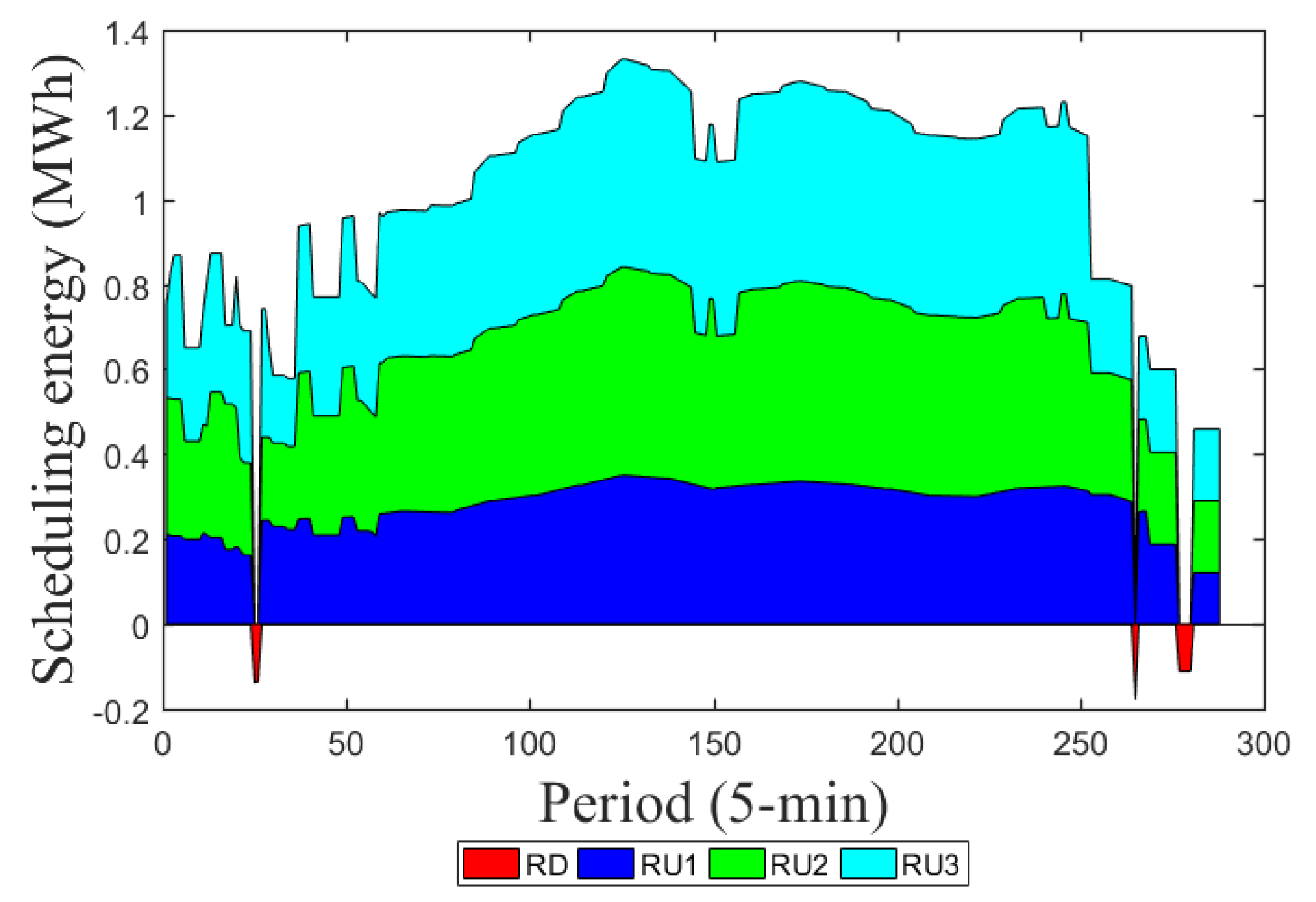
During the real-time stage, ancillary services are used to correct the imbalance that occurs in the system. At this stage, the resources deliver the power scheduled by the VPP according to the energy and reserve scheduling in the previous stage. Thus, the reserve power capacity required to balance the system is deployed in this stage. Figure 7 shows the scheduling of each type of reserve needed to balance the system. Analysing this figure, most of the periods require a need for upward reserve services, meaning more generation has been scheduled. Only a few periods used downward reserve, because the real-time demand reached a value lower to the one forecasted in intra-day. Thus, the most expensive generation resources have been reduced for matching with the real-time demand power.
The participation of each type of resource on energy and reserve for hour 10 is shown in Table 3 and Table 4. One can see that the resources scheduling changed in each stage, e.g., storage units only participate in the real-time. It is noteworthy, that the power losses in hour-ahead and real-time are lower than the day-ahead stage. This is due to the time to delivery of energy is closer, thereby forecast are more accurate allowing an improvement on the power losses. The increasing use of DER, especially ESSs, can also reduce the losses, since these resources are closer to the demand comparing to external suppliers.
5. Conclusions
The continuous large-scale penetration of distributed energy resources in electric power systems will lead to further integration of new operational and management schemes and tools for a proper operation and balance of the power system. DERs will be useful not only to participate in the energy market but also to contribute in the AS required by system operators to balance the system. For that purpose, aggregators and distributed system operators will eventually develop tools for joint optimization of energy and reserve services considering different time-horizons.
The main motivation behind this work was to formulate and to develop a tool able for simulating DER management under participation in energy and reserve services during day-ahead, hour-ahead and real-time stages of power system operation. DER participation in frequency control services, namely downward and upward reserve, were considered. These services help the VPP to balance the system. The participation of DERs in different services will help the network operators to manage the electric system under a scenario with very high penetration of renewable resources. This new paradigm represents an opportunity to the producers but also to the operators, because they can use resources with different characteristics and distributed in all network levels.
The simulation results show that the rescheduling of energy resources over the time-horizons ensures a proper operation of the power system. On one hand, the rescheduling of energy and reserve at hour-ahead stage allows the VPP to adjust the production considering the uncertainty of the resources and demand forecasts. In addition, the use of reserve to balance the system in real-time mitigates the energy deviations from hour-ahead to real-time stage. On the other hand, the use of better forecast at upstream stages could result in fewer adjustments on energy and reserve scheduling, thereby reducing the operation costs for the VPP.
Besides the main message, this work allows us to draw several conclusions. The most significant conclusions reflect that (i) most of the balance needs requires upward reserve services; (ii) energy and reserve scheduling strongly depends on uncertain generation and demand forecast; and (iii) good computer performance for simulation of large-scale management of distributed energy resources has been achieved.
Future work will focus on improving distinct factors of the developed tool. On one hand, stochastic programming may be used for dealing with uncertainty of the intermittent resources, such as wind, photovoltaic and EVs. On the other hand, the participation of DERs may be integrated in voltage control services to improve the power system reliability. In addition, different market structures considering additional constraints for DERs can be addressed. The inclusion of EVs in reserve participation is another point of interest. Finally, constrained and meshed distribution grids with high penetration of DERs can be tested and validated.
Acknowledgments
The authors would like to acknowledge Pierre Pinson for giving valuable suggestions for the paper. The post-doctoral grant of Tiago Soares was financed by the ERDF – European Regional Development Fund through the Operational Programme for Competitiveness and Internationalisation - COMPETE 2020 Programme, and by National Funds through the Portuguese funding agency, FCT - Fundação para a Ciência e a Tecnologia, within project ESGRIDS - Desenvolvimento Sustentável da Rede Elétrica Inteligente/SAICTPAC/0004/2015- POCI-01-0145-FEDER-016434. This work is partly supported by the Danish Innovation Fund through the projects ’5s’ - Future Electricity Markets (12-132636/DSF) and CITIES (DSF-1305-00027B). This work has received funding from the European Union's Horizon 2020 research and innovation programme under the Marie Sklodowska-Curie grant agreement No 641794 (project DREAM-GO) and from FEDER Funds through COMPETE program and from National Funds through FCT under the project UID/EEA/00760/2013.
Author Contributions
T. Soares, M. Silva, H. Morais and Z. Vale conceived the models presented in the paper. T. Soares and M. Silva implemented the optimization framework. T. Sousa and H. Morais performed the simulation work and analysis concerning the results. T. Soares, T. Sousa and H. Morais wrote the paper. Z. Vale proofread the paper.
Conflicts of Interest
The authors declare no conflict of interest.
Nomenclature
The main notation used throughout the paper is stated next for quick reference. Other symbols are defined as required.
Parameters
| Elementary period t duration (e.g., 15 min (0.25), 30 min (0.50)) | |
| Grid-to-Vehicle efficiency | |
| Vehicle-to-Grid efficiency | |
| Imaginary part in admittance matrix (S) | |
| Resource cost in period t (m.u./kWh) | |
| Stored energy in the battery of vehicle at the end of period t (kWh) | |
| Energy stored in the battery of vehicle at the beginning of period 1 (kWh) | |
| Energy consumption in the battery during a trip that occurs in period t (kWh) | |
| Real part in admittance matrix (S) | |
| Total number of resources | |
| Maximum apparent power (kVA) | |
| Total number of periods | |
| Set of lines connected to a certain bus | |
| Voltage in polar form (V) | |
| Penalization cost (m.u./kWh) | |
| Series admittance of line that connect two buses (S) | |
| Shunt admittance of line that connect two buses (S) |
Variables
| Voltage angle | |
| Active power (kW) | |
| Reactive power (kVAr) | |
| Relaxation variable for downward reserve (kW) | |
| Relaxation variable for upward reserve (kW) | |
| Voltage magnitude (V) | |
| Binary variable |
Indexes
| Downward reserve service | |
| Power requirement for the AS | |
| Upward reserve service | |
| Battery energy capacity | |
| Minimum stored energy to be guaranteed at the end of period t | |
| Bus | |
| Charge process | |
| Day-ahead stage | |
| Discharge process | |
| Battery degradation | |
| Distributed generation unit | |
| Forecast power of distributed generation unit in period t | |
| Demand response program for loads with continuous regulation | |
| Demand response program for loads with discrete regulation (on/off) | |
| Electric vehicle | |
| Generation curtailment power | |
| Bus i and Bus j | |
| Intraday stage | |
| Load | |
| Periods in the real-time stage | |
| Upper bound limit | |
| Lower bound limit | |
| Non-supplied demand | |
| Real-time stage | |
| Storage unit | |
| Stored energy in the battery of the vehicle for the energy and RD services | |
| Stored energy in the battery of the vehicle for the energy, RU, SP and NS services | |
| External supplier | |
| Line | |
| Total maximum limit for the resources considering the energy, RU, SP and NS services | |
| Total minimum limit for the resources considering the energy and RD services |
References
- Lund, H. Renewable Energy Systems: A Smart Energy Systems Approach to the Choice and Modeling of 100% Renewable Solutions, 2nd ed.; Elsevier: Boston, MA, USA, 2014. [Google Scholar]
- Jones, L. Renewable Energy Integration: Practical Management of Variability, Uncertainty and Flexibility in Power Grids, 1st ed.; Elsevier: Boston, MA, USA, 2014. [Google Scholar]
- Ela, E.; Kirby, B.; Navid, N.; Smith, J.C. Effective ancillary services market designs on high wind power penetration systems. In Proceedings of the 2012 IEEE Power and Energy Society General Meeting, San Diego, CA, USA, 22–26 July 2012; pp. 1–8. [Google Scholar]
- Morais, H.; Pinto, T.; Vale, Z.; Praca, I. Multilevel negotiation in smart grids for VPP management of distributed resources. IEEE Intell. Syst. 2012, 27, 8–16. [Google Scholar] [CrossRef]
- Nosratabadi, S.M.; Hooshmand, R.-A.; Gholipour, E. A comprehensive review on microgrid and virtual power plant concepts employed for distributed energy resources scheduling in power systems. Renew. Sustain. Energy Rev. 2017, 67, 341–363. [Google Scholar] [CrossRef]
- González, P.; Villar, J.; Díaz, C.A.; Campos, F.A. Joint energy and reserve markets: Current implementations and modeling trends. Electr. Power Syst. Res. 2014, 109, 101–111. [Google Scholar] [CrossRef]
- Cochran, J.; Miller, M.; Milligan, M.; Ela, E.G.; Arent, D.; Bloom, A.; Futch, M.; Kiviluoma, J.; Holttinen, H.; Orths, A. Market Evolution: Wholesale Electricity Market Design for 21st Century Power Systems; National Renewable Energy Laboratory: Washington, DC, USA, 2013.
- Soares, T.; Bessa, R.J.; Pinson, P.; Morais, H. Active Distribution Grid Management based on Robust AC Optimal Power Flow. IEEE Trans. Smart Grid 2017, PP, 1. [Google Scholar] [CrossRef]
- Burger, S.; Chaves-Ávila, J.P.; Batlle, C.; Pérez-Arriaga, I.J. The Value of Aggregators in Electricity Systems; MIT Center for Energy and Environment Policy Research: Cambridge, MA, USA, 2016. [Google Scholar]
- Morais, H.; Kádár, P.; Faria, P.; Vale, Z.A.; Khodr, H.M. Optimal scheduling of a renewable micro-grid in an isolated load area using mixed-integer linear programming. Renew. Energy 2010, 35, 151–156. [Google Scholar] [CrossRef]
- Tushar, W.; Chai, B.; Yuen, C.; Smith, D.B.; Wood, K.L.; Yang, Z.; Poor, H.V. Three-Party Energy Management With Distributed Energy Resources in Smart Grid. IEEE Trans. Ind. Electron. 2014, 62, 1–12. [Google Scholar] [CrossRef]
- Iqbal, M.; Azam, M.; Naeem, M.; Khwaja, A.S.; Anpalagan, A. Optimization classification, algorithms and tools for renewable energy: A review. Renew. Sustain. Energy Rev. 2014, 39, 640–654. [Google Scholar] [CrossRef]
- Guerrero-Mestre, V.; de la Nieta, A.A.S.; Contreras, J.; Catalão, J.P.S. Optimal Bidding of a Group of Wind Farms in Day-Ahead Markets Through an External Agent. IEEE Trans. Power Syst. 2016, 31, 2688–2700. [Google Scholar] [CrossRef]
- Haddadian, G.; Khalili, N.; Khodayar, M.; Shahidehpour, M. Optimal scheduling of distributed battery storage for enhancing the security and the economics of electric power systems with emission constraints. Electr. Power Syst. Res. 2015, 124, 152–159. [Google Scholar] [CrossRef]
- Arslan, O.; Karasan, O.E. Cost and emission impacts of virtual power plant formation in plug-in hybrid electric vehicle penetrated networks. Energy 2013, 60, 116–124. [Google Scholar] [CrossRef] [Green Version]
- Sousa, T.; Morais, H.; Castro, R.; Vale, Z. Evaluation of different initial solution algorithms to be used in the heuristics optimization to solve the energy resource scheduling in smart grids. Appl. Soft Comput. 2016, 48, 491–506. [Google Scholar] [CrossRef]
- Delfino, F.; Minciardi, R.; Pampararo, F.; Robba, M. A multilevel approach for the optimal control of distributed energy resources and storage. IEEE Trans. Smart Grid 2014, 5, 2155–2162. [Google Scholar] [CrossRef]
- Song, I.-K.; Jung, W.-W.; Kim, J.-Y.; Yun, S.-Y.; Choi, J.-H.; Ahn, S.-J. Operation Schemes of Smart Distribution Networks With Distributed Energy Resources for Loss Reduction and Service Restoration. IEEE Trans. Smart Grid 2013, 4, 367–374. [Google Scholar] [CrossRef]
- Ghafouri, A.; Milimonfared, J.; Gharehpetian, G.B. Coordinated Control of Distributed Energy Resources and Conventional Power Plants for Frequency Control of Power Systems. IEEE Trans. Smart Grid 2015, 6, 104–114. [Google Scholar] [CrossRef]
- Soares, T.; Pinson, P.; Jensen, T.V.; Morais, H. Optimal Offering Strategies for Wind Power in Energy and Primary Reserve Markets. IEEE Trans. Sustain. Energy 2016, 7, 1036–1045. [Google Scholar] [CrossRef]
- Yang, Y.; Zhai, Q.; Guan, X. An hour-ahead scheduling problem for a system with wind resource. In Proceedings of the 2012 IEEE Power and Energy Society General Meeting, San Diego, CA, USA, 22–26 July 2012; pp. 1–8. [Google Scholar]
- Ghadikolaei, H.M.; Tajik, E.; Aghaei, J.; Charwand, M. Integrated day-ahead and hour-ahead operation model of discos in retail electricity markets considering DGs and CO2 emission penalty cost. Appl. Energy 2012, 95, 174–185. [Google Scholar] [CrossRef]
- Liu, Y.; Nair, N.K.C. A Two-Stage Stochastic Dynamic Economic Dispatch Model Considering Wind Uncertainty. IEEE Trans. Sustain. Energy 2016, 7, 819–829. [Google Scholar] [CrossRef]
- Adinolfi, F.; Burt, G.M.; Crolla, P.; Agostino, F.D.; Saviozzi, M.; Silvestro, F. Distributed Energy Resources Management in a Low-Voltage Test Facility. IEEE Trans. Ind. Electron. 2015, 62, 2593–2603. [Google Scholar] [CrossRef]
- Silva, M.; Morais, H.; Vale, Z. An integrated approach for distributed energy resource short-term scheduling in smart grids considering realistic power system simulation. Energy Convers. Manag. 2012, 64, 273–288. [Google Scholar] [CrossRef]
- Salinas, S.; Li, M.; Li, P.; Fu, Y. Dynamic Energy Management for the Smart Grid with Distributed Energy Resources. IEEE Trans. Smart Grid 2013, 4, 2139–2151. [Google Scholar] [CrossRef]
- Rahbar, K.; Chai, C.C.; Zhang, R. Real-time energy management for cooperative microgrids with renewable energy integration. In Proceedings of the 2014 IEEE International Conference on Smart Grid Communications (SmartGridComm), Venice, Italy, 3–6 November 2014; pp. 25–30. [Google Scholar]
- Rahimiyan, M.; Baringo, L. Strategic Bidding for a Virtual Power Plant in the Day-Ahead and Real-Time Markets: A Price-Taker Robust Optimization Approach. IEEE Trans. Power Syst. 2016, 31, 2676–2687. [Google Scholar] [CrossRef]
- Li, H.; Li, F.; Xu, Y.; Rizy, D.T.; Adhikari, S. Autonomous and adaptive voltage control using multiple distributed energy resources. IEEE Trans. Power Syst. 2013, 28, 718–730. [Google Scholar] [CrossRef]
- Shahnia, F.; Chandrasena, R.P.S.; Rajakaruna, S.; Ghosh, A. Primary control level of parallel distributed energy resources converters in system of multiple interconnected autonomous microgrids within self-healing networks. Gener. Transm. Distrib. IET 2014, 8, 203–222. [Google Scholar] [CrossRef]
- Kulmala, A.; Repo, S.; Järventausta, P. Coordinated Voltage Control in Distribution Networks Including Several Distributed Energy Resources. IEEE Trans. Smart Grid 2014, 5, 1–11. [Google Scholar] [CrossRef]
- Silva, M.; Morais, H.; Sousa, T.; Vale, Z. Energy resources management in three distinct time horizons considering a large variation in wind power. In Proceedings of the European Wind Energy Conference & Exhibition 2013, Vienna, Austria, 4–7 February 2013. [Google Scholar]
- Zakariazadeh, A.; Jadid, S.; Siano, P. Economic-environmental energy and reserve scheduling of smart distribution systems: A multiobjective mathematical programming approach. Energy Convers. Manag. 2014, 78, 151–164. [Google Scholar] [CrossRef]
- Mohan, V.; Singh, J.G.; Ongsakul, W. An efficient two stage stochastic optimal energy and reserve management in a microgrid. Appl. Energy 2015, 160, 28–38. [Google Scholar] [CrossRef]
- Ferreira, J.; Monteiro, V.; Afonso, J. Vehicle-to-Anything Application (V2Anything App) for Electric Vehicles. IEEE Trans. Ind. Inform. 2013, 10, 1927–1937. [Google Scholar] [CrossRef]
- Soares, J.; Canizes, B.; Lobo, C.; Vale, Z.; Morais, H. Electric vehicle scenario simulator tool for smart grid operators. Energies 2012, 5, 1881–1899. [Google Scholar] [CrossRef]
- Vecchietti, A.; Grossmann, I.; Raman, R.; Kalvelagen, E. DICOPT Solver; Carnegie Mellon University, and GAMS Development Corporation: Pittsburgh, PA, USA, 2008. [Google Scholar]
- Rosenthal, R. GAMS—A User’s Guide; GAMS Development Corporation: Washington, DC, USA, 2008. [Google Scholar]
- Peterson, S.B.; Whitacre, J.F.; Apt, J. The economics of using plug-in hybrid electric vehicle battery packs for grid storage. J. Power Sources 2010, 195, 2377–2384. [Google Scholar] [CrossRef]
Figure 1.
Timeline optimization of the proposed model.
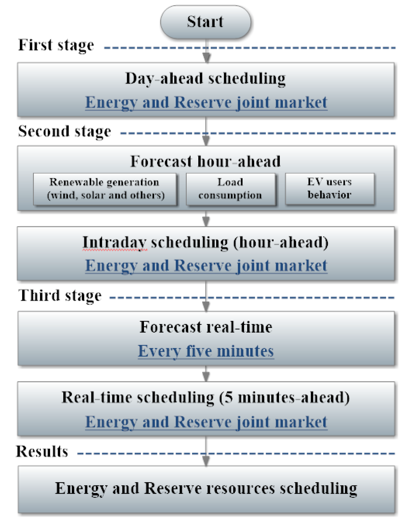
Figure 2.
Intraday (hour-ahead) scheduling diagram.
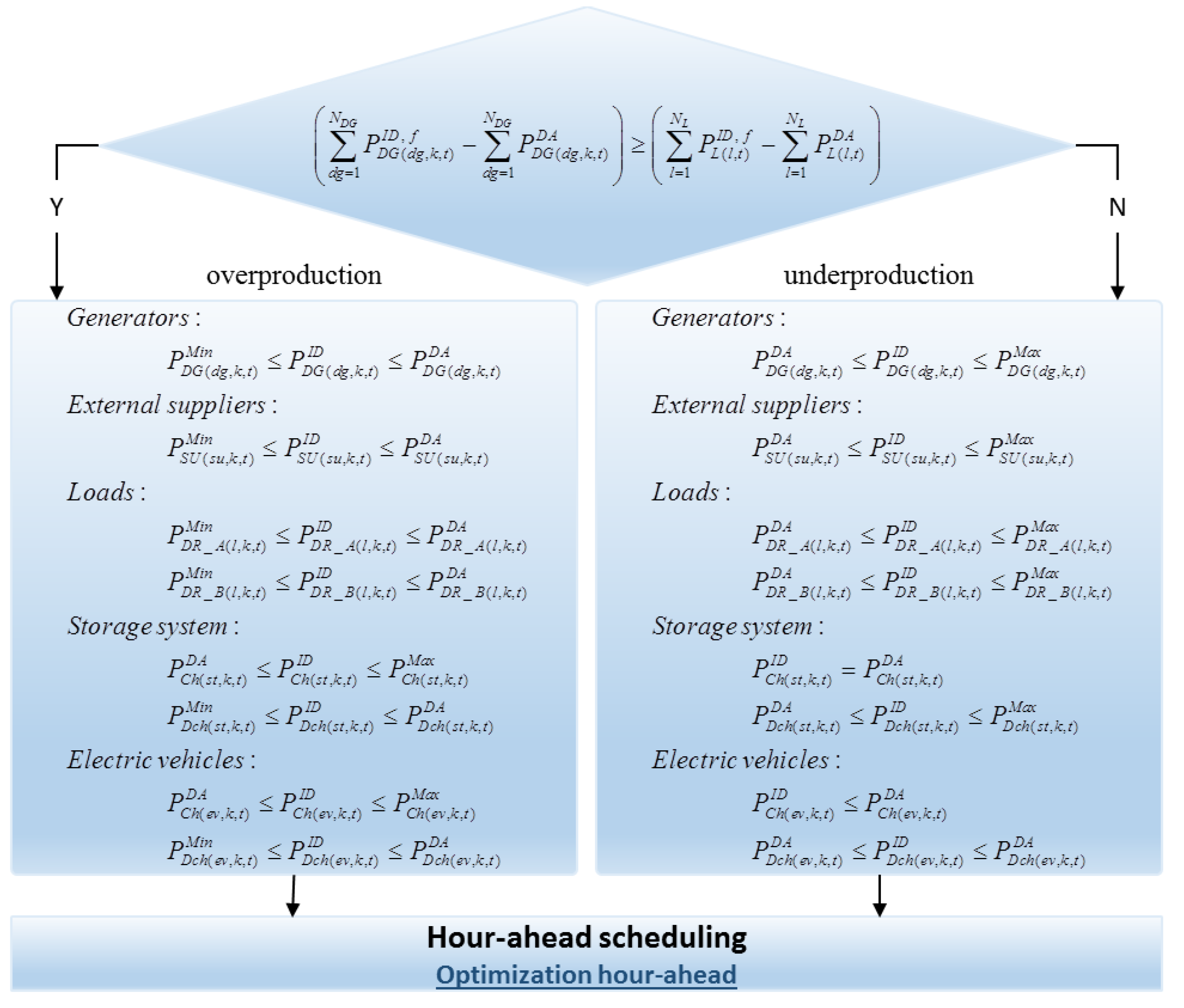
Figure 3.
Thirty-three-bus network configuration (reprint with permission [25]; 2012, Elsevier).
Figure 3.
Thirty-three-bus network configuration (reprint with permission [25]; 2012, Elsevier).
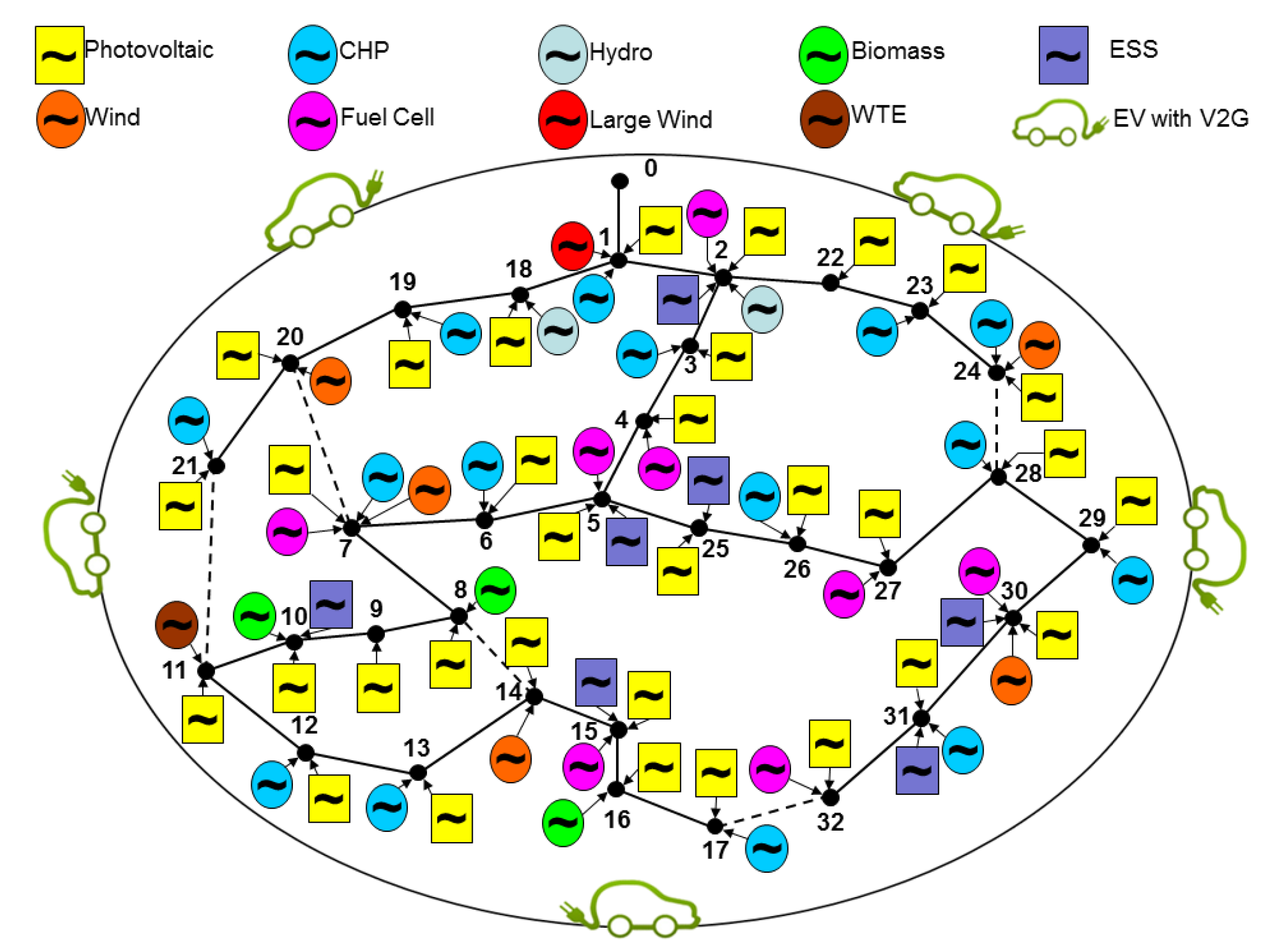
Figure 4.
Energy scheduling at day-ahead, hour-ahead and real-time stages.
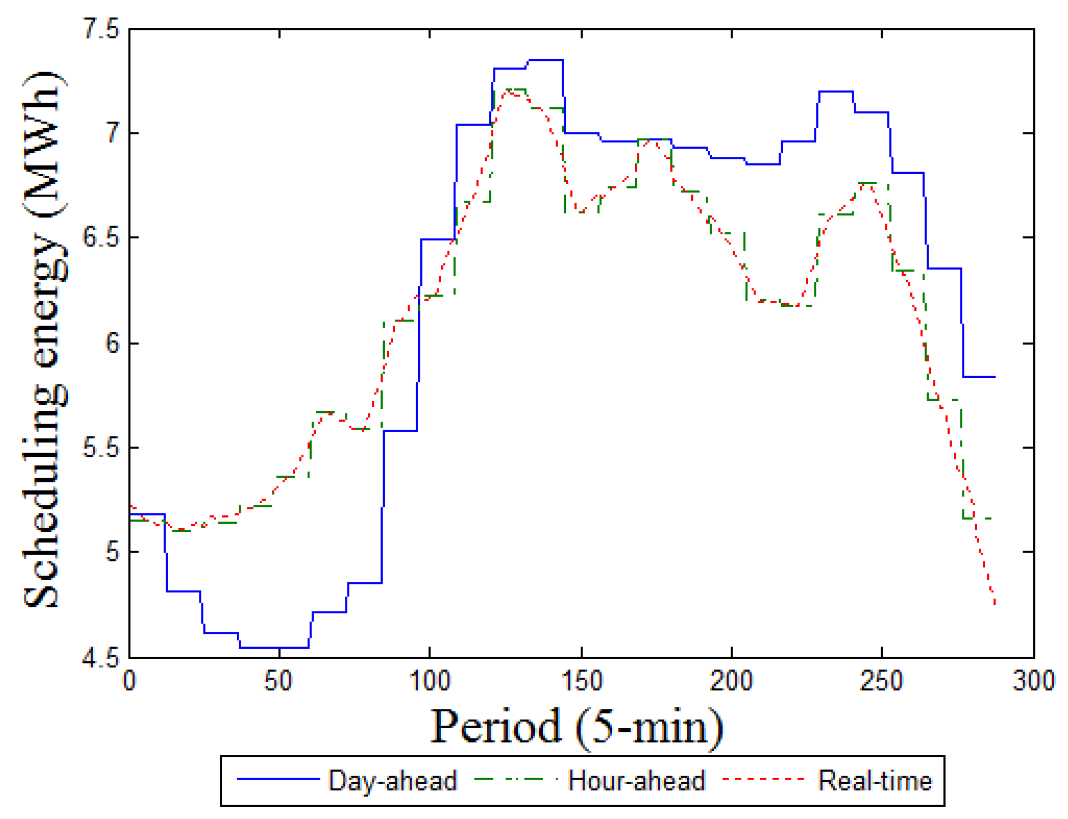
Figure 5.
Reserve capacity scheduling at day-ahead stage.

Figure 6.
Reserve capacity rescheduling at hour-ahead stage.
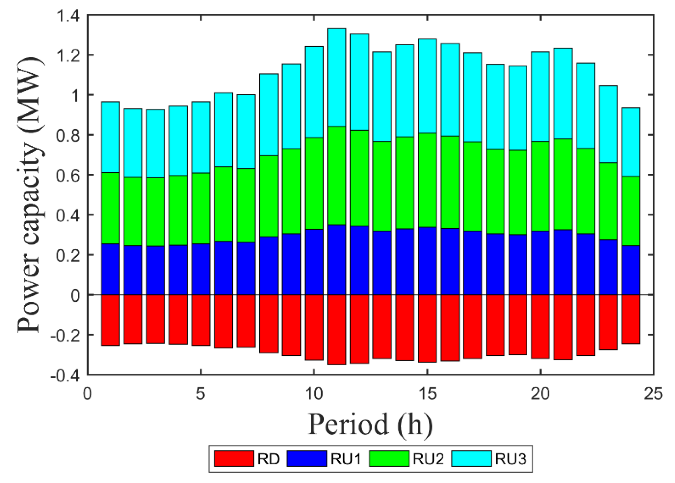
Figure 7.
Reserve services used to balance the system in real-time.

Table 1.
Energy resources data.
| Energy Resources | Availability (kW) Min–Max | Prices (m.u./kWh) | |
|---|---|---|---|
| Biomass | 0–375 | 0.09 | |
| CHP | 0–1150 | 0.06 | |
| Fuel cell | 0–210 | 0.09 | |
| Small hydro | 0–70 | 0.07 | |
| Photovoltaic | 0–837 | 0.20 | |
| Waste-to-energy | 0–10 | 0.10 | |
| Small wind | 182–891 | 0.15 | |
| Large wind | 2000–5000 | 0.07 | |
| External supplier | 0–6200 | 0.06–0.15 | |
| Storage | Charge | 0–1050 | 0.09–0.16 |
| Discharge | 0–700 | 0.11–0.18 | |
| Electric vehicle | Charge | 0–6305 | 0.09–0.16 |
| Discharge | 0–6616 | 0.20 | |
| Demand response | Red | 0–1731 | 0.150–0.160 |
| Cut | 0–831 | 0.160 | |
| Consumers demand | 4251–7451 | 0.14 | |
Table 2.
Resources data for all reserve services.
| Energy Resources | Power (kW) | Price (m.u./kWh) | ||||
|---|---|---|---|---|---|---|
| [RD, RU_1] | [RU_2, RU_3] | [RD, RU_1] | RU_2 | RU_3 | ||
| Biomass | 0–18.8 | 0–26.3 | 0.099 | 0.108 | 0.116 | |
| CHP | 0–57.5 | 0–80.5 | 0.066 | 0.072 | 0.078 | |
| Fuel cell | 0–10.5 | 0–14.7 | 0.099 | 0.108 | 0.116 | |
| Small hydro | 0–3.5 | 0–4.9 | 0.077 | 0.084 | 0.090 | |
| Photovoltaic | 0–41.9 | 0–58.6 | 0.220 | 0.240 | 0.260 | |
| Waste-to-energy | 0–0.5 | 0–0.7 | 0.110 | 0.120 | 0.130 | |
| Small wind | 9.1–44.6 | 12.7–62.4 | 0.165 | 0.180 | 0.194 | |
| Large wind | 100–250 | 140–350 | 0.077 | 0.084 | 0.090 | |
| External supplier | 0–310 | 0–434 | 0.115 | 0.126 | 0.136 | |
| Storage | Charge | 0–1050 | 0.145 | 0.158 | 0.172 | |
| Discharge | 0–700 | 0.168 | 0.183 | 0.198 | ||
| Demand response | Red | 0–173.1 | 0–121.2 | 0.168 | 0.183 | 0.198 |
| Cut | 0–41.6 | 0–58.2 | 0.176 | 0.192 | 0.208 | |
Table 3.
Energy and reserve scheduling on hour 10 for day-ahead and hour-ahead stage.
| Energy Resources | Day-Ahead (MW) | Hour-Ahead (MW) | |||||||||
|---|---|---|---|---|---|---|---|---|---|---|---|
| Energy | RD | RU_1 | RU_2 | RU_3 | Energy | RD | RU_1 | RU_2 | RU_3 | ||
| Biomass | 0.304 | 0.019 | 0.019 | 0.026 | 0.026 | 0.338 | 0.019 | 0 | 0.011 | 0.026 | |
| CHP | 0.932 | 0.058 | 0.058 | 0.081 | 0.081 | 0.951 | 0.058 | 0.038 | 0.080 | 0.081 | |
| Fuel cell | 0.077 | 0.011 | 0.002 | 0.001 | 0.006 | 0.210 | 0.011 | 0 | 0 | 0 | |
| Small hydro | 0.057 | 0.004 | 0.004 | 0.005 | 0.005 | 0.057 | 0.004 | 0.004 | 0.005 | 0.005 | |
| Photovoltaic | 0.180 | 0 | 0 | 0 | 0 | 0.144 | 0 | 0 | 0 | 0 | |
| Waste-to-energy | 0.008 | 0.001 | 0.001 | 0.001 | 0.001 | 0.009 | 0.001 | 0 | 0 | 0.001 | |
| Small wind | 0.182 | 0 | 0 | 0 | 0 | 0.146 | 0 | 0 | 0 | 0 | |
| Large wind | 4.500 | 0 | 0 | 0 | 0 | 1.350 | 0 | 0 | 0 | 0 | |
| External supplier | 2.450 | 0.246 | 0.190 | 0.358 | 0.267 | 3.534 | 0.236 | 0.193 | 0.266 | 0.266 | |
| Storage | Charge | 0 | 0 | 0 | 0 | 0 | 0 | 0 | 0 | 0 | 0 |
| Electric vehicles (EV) | Discharge | 0 | 0 | 0 | 0 | 0 | 0 | 0 | 0 | 0 | 0 |
| Charge | 1.771 | - | - | - | - | 1.771 | - | - | - | - | |
| Discharge | 0 | - | - | - | - | 0 | - | - | - | - | |
| Demand response (DR) | Red | 0.123 | 0 | 0.064 | 0 | 0.086 | 1.331 | 0 | 0.092 | 0.096 | 0.079 |
| Cut | 0 | 0 | 0 | 0 | 0 | 0.368 | 0 | 0 | 0 | 0 | |
| Consumers demand | 6.740 | 0 | 0 | 0 | 0 | 6.537 | 0 | 0 | 0 | 0 | |
| Power losses | 0.3018 | 0.131 | |||||||||
| AS requirement | - | 0.337 | 0.337 | 0.472 | 0.472 | - | 0.327 | 0.327 | 0.458 | 0.458 | |
Table 4.
Energy and reserve scheduling on hour 10 in real-time stage.
| Energy Resources | Real-Time (MW) | |||||
|---|---|---|---|---|---|---|
| Energy | RD | RU_1 | RU_2 | RU_3 | ||
| Biomass | 0.338 | 0 | 0 | 0.011 | 0.026 | |
| CHP | 0.951 | 0 | 0.014 | 0.078 | 0.078 | |
| Fuel cell | 0.210 | 0 | 0 | 0 | 0 | |
| Small hydro | 0.057 | 0 | 0.004 | 0.005 | 0.005 | |
| Photovoltaic | 0.229 | 0 | 0 | 0 | 0 | |
| Waste-to-energy | 0.009 | 0 | 0 | 0 | 0.001 | |
| Small wind | 0.147 | 0 | 0 | 0 | 0 | |
| Large wind | 1.566 | 0 | 0 | 0 | 0 | |
| External supplier | 3.478 | 0 | 0.178 | 0.266 | 0.266 | |
| Storage | Charge | 0.042 | 0 | 0.042 | 0 | 0 |
| Discharge | 0 | 0 | 0 | 0 | 0 | |
| EV | Charge | 1.771 | - | - | - | - |
| Discharge | 0 | - | - | - | - | |
| DR | Red | 1.354 | 0 | 0.092 | 0.092 | 0.079 |
| Cut | 0.187 | 0 | 0 | 0 | 0 | |
| Consumers demand | 6.577 | 0 | 0 | 0 | 0 | |
| Power losses | 0.137 | |||||
| AS requirement | - | 0 | 0.329 | 0.460 | 0.460 | |
© 2017 by the authors. Licensee MDPI, Basel, Switzerland. This article is an open access article distributed under the terms and conditions of the Creative Commons Attribution (CC BY) license (http://creativecommons.org/licenses/by/4.0/).
Share and Cite
MDPI and ACS Style
Soares, T.; Silva, M.; Sousa, T.; Morais, H.; Vale, Z. Energy and Reserve under Distributed Energy Resources Management—Day-Ahead, Hour-Ahead and Real-Time. Energies 2017, 10, 1778. https://doi.org/10.3390/en10111778
AMA Style
Soares T, Silva M, Sousa T, Morais H, Vale Z. Energy and Reserve under Distributed Energy Resources Management—Day-Ahead, Hour-Ahead and Real-Time. Energies. 2017; 10(11):1778. https://doi.org/10.3390/en10111778
Chicago/Turabian StyleSoares, Tiago, Marco Silva, Tiago Sousa, Hugo Morais, and Zita Vale. 2017. "Energy and Reserve under Distributed Energy Resources Management—Day-Ahead, Hour-Ahead and Real-Time" Energies 10, no. 11: 1778. https://doi.org/10.3390/en10111778
Note that from the first issue of 2016, this journal uses article numbers instead of page numbers. See further details here.