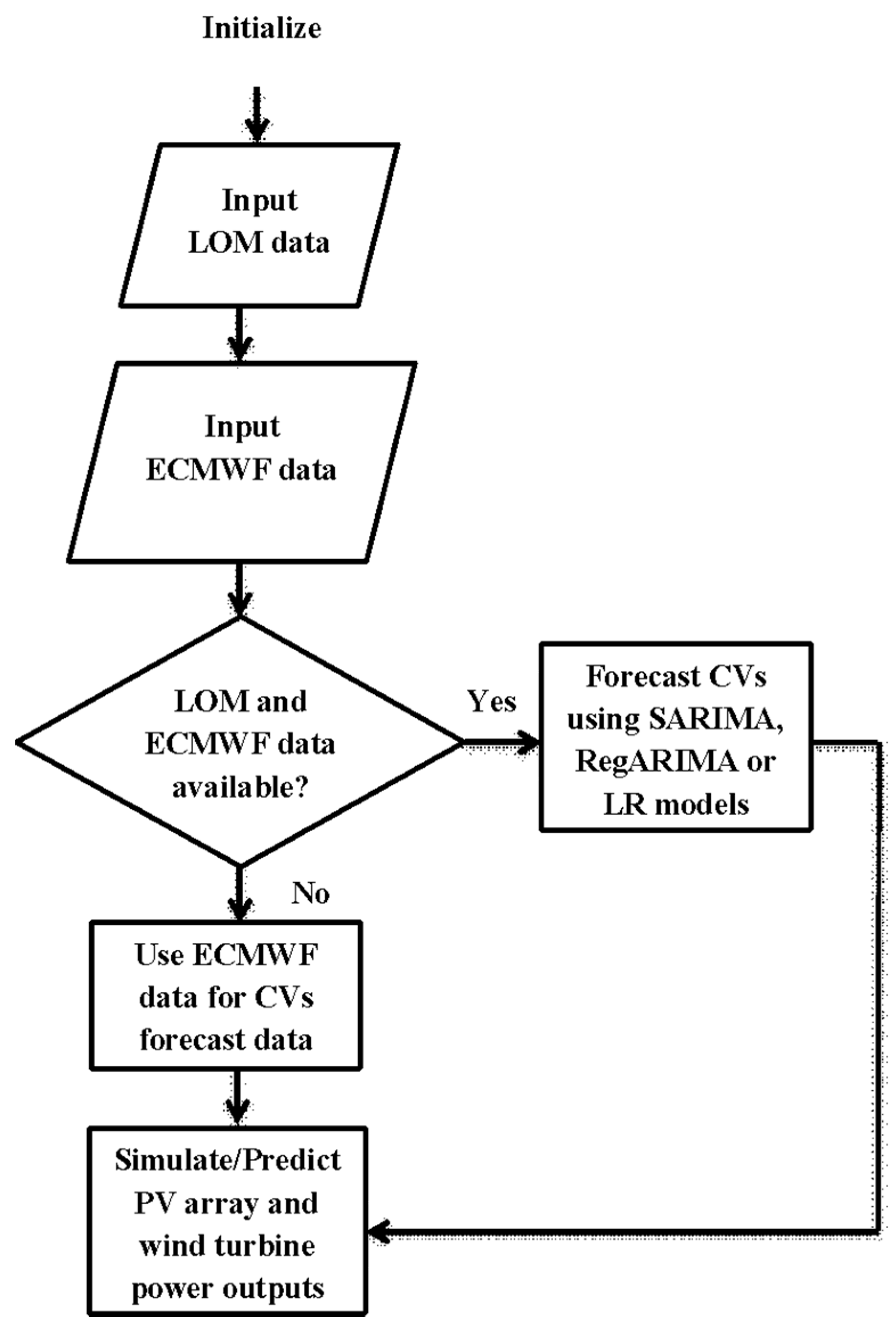
Article

A Decision Support Tool for Building Integrated Renewable Energy Microgrids Connected to a Smart Grid

Department of Process, Energy and Transport Engineering, Cork Institute of Technology, Co. Cork T12 P928, Ireland
*
Author to whom correspondence should be addressed.
Energies 2017, 10(11), 1765; https://doi.org/10.3390/en10111765
Submission received: 11 August 2017 / Revised: 15 October 2017 / Accepted: 23 October 2017 / Published: 2 November 2017
(This article belongs to the Section L: Energy Sources)

Abstract

:
The objective of this study was to create a tool that will enable renewable energy microgrid (REμG) facility users to make informed decisions on the utilization of electrical power output from a building integrated REμG connected to a smart grid. A decision support tool for renewable energy microgrids (DSTREM) capable of predicting photovoltaic array and wind turbine power outputs was developed. The tool simulated users’ daily electricity consumption costs, avoided CO2 emissions and incurred monetary income relative to the usage of the building integrated REμG connected to the national electricity smart grid. DSTREM forecasted climate variables, which were used to predict REμG power output over a period of seven days. Control logic was used to prioritize supply of electricity to consumers from the renewable energy sources and the national smart grid. Across the evaluated REμG electricity supply options and during working days, electricity exported by the REμG to the national smart grid ranged from 0% to 61% of total daily generation. The results demonstrated that both monetary saving and CO2 offsets can be substantially improved through the application of DSTREM to a REμG connected to a building.

1. Introduction

The use of building integrated renewable energy microgrids (REμG) has in recent years become an effective means of providing renewable energy while offsetting greenhouse gas emissions for residential and commercial consumers. Optimizing the energy utilization from REμGs has become an area of significant research interest. The creation of a decision support tool would be useful for REμG users to optimize their energy utilization from renewable sources, taking into account REμG power output, building electricity consumption, electricity tariff (ET) structures, feed-in tariff (FIT) structures, and CO2 emissions.
One important consideration in the creation of such a decision support tool is the fact that accurate predictions of climatic variables are required to simulate REμG power output. Several studies have been carried out regarding the prediction of climatic variables and simulation of renewable energy output power. REμG electricity consumption, electricity pricing structures, FIT structures and associated CO2 emissions have also been modeled and analyzed in previous research. Soshinskaya et al. [1] utilized measured wind speed, solar irradiation and real time manufacturer’s data to model a REμG serving a water treatment plant in the Netherlands. Li et al. [2] used autoregressive integrated moving average with exogenous input (ARIMAX) modeling to forecast PV power. The study showed that the forecasting accuracy of PV power output was greatly improved by the ARIMAX model when compared with an autoregressive integrated moving average model without exogenous inputs (ARIMA). Murphy et al. [3] used weather predictions from the European Centre for Medium-Range Weather Forecasts (ECMWF) and corresponding onsite empirical temperature data to generate a rolling onsite temperature forecast with a one-hour resolution. This was accomplished by using a Non-linear Auto Regressive with eXogenous input (NARX) recurrent dynamic neural network model. A significant increase in localized temperature forecast accuracy was found, which enabled the optimization of cold energy storage in a smart grid environment. A model for electricity consumption on dairy farms was created by Upton et al. [4]. This model was used to simulate annual electricity consumption along with related CO2 emissions and electricity costs on dairy farms. The model demonstrated that moving from a day and night ET structure to a flat ET structure for a dairy farm resulted in significant electricity cost increases. Impacts of electricity pricing structures on REμGs have also been studied in [5,6,7,8,9,10,11,12,13,14,15,16,17] and it has generally been found that exposing electricity consumers to variable ET structures encourages demand response and promotes demand side management. FIT policies have proven successful in the growth of renewable energy implementations [8,16,17,18,19,20]. Li et al. [21] developed and validated energy forecasting models for a building cluster with multiple buildings and distributed energy systems, while also creating a collaborative operation framework to determine the optimal operation strategies of said building cluster. Several studies have focused on smart grids and REμGs for the purpose of reducing energy consumption, costs and carbon footprint. Stamatescu et al. [22] applied a rule based control system to a microgrid under two scenarios: a domestic dwelling with low energy demand and an office building with high energy demand. In both scenarios introducing the control system resulted in improved energy efficiency and improved renewable energy utilization. Pascual et al. [23] proposed an energy management strategy for a residential REμG comprised of PV panels and a wind turbine. The proposed control strategy used battery state of charge, power at each REμG node, electrical load and renewable generation forecasts as inputs. By using forecasted data and correcting any forecasting errors according to the state of the battery, the strategy resulted in a better grid power profile when compared with other state-of-the-art strategies.
While previous studies have focused on the operations and analysis of specific renewable energy systems, localized weather forecasting, demand side management and multiple tariff based smart grids, this study focuses on developing a holistic decision support tool that may be applied to any building in any location with a standard REμG and grid connection. It is clear from the studies listed above that a holistic decision support tool for optimizing the utilization of a REμG connected to a building and the smart grid, with multiple ET structures and FITs available, may yield both monetary savings and CO2 offsets. To achieve this, scalable REμG and building models are required to allow application of the decision support tool to various building and REμG sizes. A portable weather forecasting tool is necessary to enable localized REμG power output predictions for specific building locations. A smart grid model to simulate dynamic pricing structures and FITs would enable the selection of the optimum operating strategy relative to the building load and REμG power output. A control system to manage the flow of electricity between the REμG, building and smart grid would also be required. The combination of the above sub-systems would provide a comprehensive decision support tool for optimizing energy utilization in REμGs.
The objective of this study was to develop and demonstrate a Decision Support Tool for Renewable Energy Microgrids (DSTREM). DSTREM enables the users of buildings with integrated REμGs and smart grid connections to compare different ETs, FITs, monetary income and associated CO2 emissions under different renewable energy system scenarios. To simulate the power output of the REμG, scalable mechanistic models of the PV array, wind turbine and building load profile were constructed. Three time series modeling techniques for the prediction of climate variables were simulated and validated using ECMWF forecasts and localized historical recording as training inputs. Control logic was then applied to the REμG, this creating the decision support tool. Section 2 details the construction of the weather and REμG modes, while Section 3 demonstrates the use of the model by applying it to a low energy building with an integrated REμG and a smart grid connection. Electricity costs, monetary income and avoided CO2 were further evaluated using three ET structures, three FITs and a dynamic CO2 intensity profile.

2. Materials and Methods

2.1. Climate Model Data

In this study, hourly temperature (°C) and wind speed (m/s) data were obtained from Cork airport meteorological station for seven months (January, February, March, April, May, July, and September) in the year 2013. According to the Irish calendar, winter, spring, summer and autumn begin in November, February, May and August, respectively. Hence, the climate data for the months listed took into account the climatic variations associated with each season. The seven months were selected based on the availability of data for the case study year. Corresponding hourly irradiance (W/m2) data were obtained from the National Build Energy Retrofit Test-bed (NBERT) meteorological station for the seven months mentioned. ECMWF historical temperature, wind speed and irradiance forecasts were extracted from the ECMWF database (NWP model) for the nearest grid point to Cork Institute of Technology (CIT), approximately 2.58 km north of the base point. The data obtained from NBERT meteorological station in a resolution of one hour were split into two groups; one for model training and the other for validation and demonstration purposes. Seven weeks of climatic data, each representing one of the seven months listed above, were employed for validation while one of the seven weeks was selected as a demonstration week for DSTREM analysis. As the forecast horizon was based on a typical working week, the last seven days of each month were selected as the demonstration dataset and were used for model validation. Simulating over a longer period was beyond the scope of this study. ECMWF forecasts for temperature, irradiance and wind speed were based on a three-hour resolution. These forecasts were separated into hourly intervals through interpolation in order to synchronize with the corresponding observed data.
The last seven days of each month were selected as the target periods for all three weather variables. Twenty-one days of preceding data were used to train the models for each weather variable. This training duration (21 days) was found to yield the optimal results. The 21 days of input data contained hourly records for each weather parameter (temperature (°C), wind speed (m/s) and irradiance (W/m2)) and the corresponding ECMWF forecast values for each parameter. Therefore, the regression models (see Section 2.2) were trained based on the forecast error of the ECMWF relative to the actual values (local empirical records) of the weather parameters at a specific time (hourly) over the preceding 21 days. This input data arrangement allowed the regression models to map the relationship between the ECMWF forecast and the actual recorded parameters at specific times of the day. Therefore, if there were reoccurring errors in the ECMWF forecast the regression models could be applied as calibration tools to reduce the magnitude of the ECMWF error. This methodology has been successfully employed in cognate studies [3,24,25]. The DSTREM seven-day forecast was then generated by receiving the ECMWF forecast for the seven-day period and feeding this information into the regressions models to generate a calibrated forecast. In situations where ECMWF forecasts could not be obtained, actual values (local empirical records) alone were used to generate the DSTREM forecast (see Figure 1). The improvement in weather parameter prediction accuracy is displayed in Section 3.1.

2.2. Climatic Variables Prediction Models

2.2.1. Seasonal Autoregressive Integrated Moving Average Model

The ARIMA model is a forecasting technique that simulates future values of a time series based on historic data. The application of the ARIMA methodology for the study of time series analysis was proposed by Box and Jenkins [26]. Its main assumption is that a time series’ own past values can be used to predict its current value.
In this paper, a variation of the standard ARIMA model, the seasonal ARIMA model (SARIMA), was used to account for the inherent seasonal (24 h) effect of the analyzed climatic variables. The model is generally referred to as SARIMA (p d q) x (P D Q)s, where p, d, q and P, D, Q are non-negative integers that refer to the polynomial order of the autoregressive, integrated, and moving average parts of the non-seasonal and seasonal components of the model, respectively, while s represents the seasonality factor of the variable [27].
The SARIMA model is represented mathematically as:
φ p ( B )   Φ P ( B s ) d   s D y t = θ q ( B )   Θ Q ( B s ) ε t ,
where y t is the forecast variable (temperature, irradiance or wind speed), s defines the seasonal period of the time series, φ p ( B ) and θ q ( B ) represent the regular autoregressive and moving average polynomial components of order p and q respectively, Φ P ( B s ) and Θ Q ( B s ) represent the seasonal autoregressive and moving average polynomial components of order P and Q, respectively. The differentiating operator d and the seasonal differentiating operator s D eliminate the non-seasonal and seasonal non-stationarity, respectively. B is the backshift operator, which operates on the observation y t by shifting it one point in time and term ϵ t follows a white noise process. The expressions are defined mathematically as follows:
φ p ( B ) = 1 φ 1 B φ 2 B 2 φ p B p ,
Φ P ( B ) = 1 Φ 1 B s Φ 2 B 2 s Φ P B P s ,
θ q ( B ) = 1 + θ 1 B + θ 2 B 2 + + θ q B q ,
Θ Q ( B ) = 1 + Θ 1 B s + Θ 2 B 2 s + + Θ Q B Q s ,
d = ( 1 B ) d ,
s D = ( 1 B s ) D ,
B k ( y t ) = y t k , .
The model’s development consisted of four iterative steps: Identification, estimation, diagnostic checking and forecasting [26]. The models were created in MATLAB (Version 8.1, MathWorks, Inc., Natick, MA, USA) which uses a maximum likelihood estimation method, while the selection of the most appropriate model for each simulation was based on automatically selecting a model with the minimum Bayesian information criterion [26].

2.2.2. Linear Regression Model

The standard linear regression (LR) model is of the form:
y = b x + ϵ ,
where y is the forecast variable (observed data), x is the independent or explanatory variable (ECMWF data in this study), b is the regression coefficient and ϵ is the error term.

2.2.3. Regression Model with ARIMA Errors

Regression model with ARIMA errors (RegARIMA) is a time series modeling technique with two components: a regression model and an error model. The regression coefficients are automatically generated based on the input training data. More details on the modeling technique can be found in [28]. RegARIMA explains the behavior of a response using a linear regression model with predictor data, though the errors have autocorrelation indicative of an ARIMA process. The model is of the form:
y t = c + X t β + u t ,
a ( L )   A ( L ) ( 1 L ) D ( 1 L s ) u t = b ( L )   B ( L ) ε t ,
where t = 1, …, T, yt is the forecast variable, Xt is the predictor data at time t, C is the regression model intercept, β is the regression coefficient, ut is the disturbance series, εt is the innovative series, (1 − L)D is the degree D non-seasonal integration polynomial, and (1 − Ls) is the degree s seasonal integration polynomial. The degree p non-seasonal autoregressive polynomial a(L) is expressed as follows:
a(L) = (1a1L − … − apLp).
The degree ps seasonal autoregressive polynomial A(L) is expressed as follows:
A(L) = (1A1L − … − ApsLps).
The degree q non-seasonal moving average polynomial b(L) is expressed as follows:
b(L) = (1 + b1L + … + bqLq).
The degree qs seasonal moving average polynomial B(L) is expressed as follows:
B(L) = (1 + B1L + … + BqsLqs).

2.2.4. Statistical Validation

To compare the forecast to the validation dataset and verify the prediction accuracy of the proposed time series models for prediction of temperature, irradiance and wind speed, three forecast statistical error measures were employed; Mean Week Error (MWE), Root Mean Square Error (RMSE) and Mean Absolute Percentage Error (MAPE).
When yt is the actual observation for a time period t and ft is the forecasted value for the same period, then the error e t , MWE, RMSE and MAPE are expressed as:
e t = y t f t ,
MWE = ( t = 1 N e t y t ) 100 ,
RMSE = t = 1 N ( e t ) 2 N ,
MAPE = t = 1 N | e t | / y t N ,
where N is the forecast time horizon (168 h in this study).

2.3. Climatic Variables Model Selection for Renewable Energy Microgrid Model

In this study, there were four different climatic variable forecast models: ECMWF, SARIMA, LR and RegARIMA. These forecast models were used to forecast climatic variables seven days ahead. Data configuration of the climatic variables is described in Section 2.1, while validation of the four forecast models were carried out using the statistical validation methods described in Section 2.2.4.
The climatic variables used as inputs for the REμG model selection process are such that in locations where there is no access to local meteorological data, the ECMWF forecasts will be solely utilized in the absence of a localized calibration technique (using close proximity empirical meteorological data). In locations where local meteorological data are available, DSTREM users can generate their own climatic variable forecast, solely using empirical data and SARIMA models, or using both ECMWF forecast and empirical data with LR or RegARIMA modeling techniques. A major characteristic of the regression models (LR and RegARIMA) is that they map the relationship between ECMWF forecasts and the corresponding local data, while the SARIMA model’s major characteristic is that it generates forecasts based on the historical patterns in the localized empirical data. Hence, the methodology described in this paper is portable and could potentially be used anywhere in the world. Figure 1 illustrates the REμG climate variable input selection process. Where CV denotes climate variable and LOM represents locally obtained meteorological data.

2.4. Renewable Energy Microgrid Models

Three renewable energy power supply scenarios were explored, namely PV, Wind and PV+Wind. In the PV scenario, REμG power output was only represented by PV power output predictions. In the Wind scenario, REμG power output was only represented by wind turbine power predictions. In the PV+Wind scenario, REμG power output was represented by the summation of PV power output and wind turbine power output predictions.

2.4.1. PV Model

This paper employed the simulation and validation methods proposed by Breen et al. [12] to model a 12 kW PV system. PV panel parameters and empirical data from the NBERT PV array were used in [12] for development and validation of the model. This model utilized the equivalent circuit of a PV cell [29,30,31,32,33,34,35] consisting of a current source and a single diode with no series or shunt resistances. It used the following expressions to determine voltage, current and power of a PV cell at maximum power point:
V m = n N s k B T q ln ( n N s k B T q I o I s c V o c ) ,
I m = I p h + I o ( n N s k B T q I s c V o c ) ,
P m = V m I m ,
where P m is the power at maximum power point (W), V m is voltage at maximum power point (V), I m is current at maximum power point (A), n is diode quality coefficient, N s is the number of cells in series in one module, k B is the Boltzmann constant (J/K), T is cell temperature (K), q is charge on the electron (C), Io is saturation current (A), Isc is short circuit current (A), Voc is open circuit voltage (V) and Iph is photocurrent (A).
Inputs to this model included specifications from the PV panel manufacturer’s datasheet [36]. For simulation purposes, temperature and irradiance inputs were obtained from the forecast results of climate variable prediction models described in Section 2.2.

2.4.2. Wind Turbine Model

For this study, the manufacturer’s power curve for a Bergey XL1 [37] was used to simulate wind turbine power output. A sixth order polynomial was fitted to the manufacturer’s data, represented in Equation (23) below:
Ƥ = f r 6 + g   r 5 + h r 4 + k r 3 + m r 2 + n r + w ,
where Ƥ is the wind turbine power output (W), r is wind speed (m/s), f, g, h, k, m, n, and w are regression coefficients equal to −0.000000711, 0.000005261, −0.001401, 0.01556, −0.05951, 0.07682 and −0.01172, respectively. The goodness of fit of the polynomial resulted in a SSE of 0.015, an R2 of 0.997 and a RMSE of 0.028 kW.
Hourly wind speed values were obtained from the climatic variable prediction model forecasts. These wind speed values were scaled to a height of 18 m using the Hellman exponential law [38] with a reference height of 10 m. This method is represented mathematically as:
r 2 = r 1 ( H 2 H 1 ) α ,
where H1 is the reference height (m), H2 is the height of the wind speed to be determined, r1 is the forecasted wind speed at height H1, r2 is the wind speed to be determined, and α is the Hellman exponent, which is a topographical function of the local site.
It should be noted that any wind turbine could be used for this analysis. Most wind turbine manufacturers publish their power curves online and thus only the regression coefficients are required for a wind turbine to be used for a similar analysis.

2.5. Microgrid Load Control

DSTREM used a load priority control algorithm on the REμG to prioritize supply of electricity to the office building. Grid priority control [7,39] was also evaluated to enable DSTREM users to make CO2 and monetary cost comparisons between usage of renewable energy supply and national smart grid power supply. Load priority dictated that electricity requirement of the office building’s occupants was prioritized to be met by the REμG power output (PV, Wind or PV+Wind scenarios), while excess electricity from the REμG was sold to the national smart grid at selected FITs (FITs described in Section 2.6.2 below). At periods when electricity production from the REμG was less than the electricity requirements of the office building, the additional required electricity was supplied by the national smart grid. The electricity requirement and the REμG power output at jth hour of the ith day of the analyzed seven days are denoted by E l o a d ( i , j ) and M G p ( i , j ) , respectively. Daily electricity supplied by the REμG is denoted by E S M G , daily electricity supplied by the national smart grid is denoted by E S G and daily electricity exported to the national smart grid is denoted by E e x . Daily electricity supplied by the REμG was computed as:
E S M G = ( j = 1 24 E m ( i , j ) ) PV , Wind , PV + Wind ,
where E m ( i , j ) is the electricity supplied by the REμG on Day i ( i = 1 7 ) and Hour j ( j = 1–24) and derived as follows:
E m ( i , j ) = { E l o a d ( i , j ) ,| M G p ( i , j ) E l o a d ( i , j ) M G p ( i , j ) ,| M G p ( i , j ) < E l o a d ( i , j ) .
Daily electricity supplied by the national smart grid was computed as:
E S G = ( j = 1 24 E g ( i , j ) ) PV , Wind , PV + Wind ,
where E g ( i , j ) is the electricity supplied by national smart grid on Day i and Hour j and derived as follows:
E g ( i , j ) = { E l o a d ( i , j ) M G p ( i , j ) ,| E l o a d > M G p 0 ,| E l o a d M G p .
Daily electricity exported to the national smart grid was computed as follows:
E E X = ( j = 1 24 E e x ( i , j ) ) PV , Wind , PV + Wind ,
where E e x ( i , j ) is the electricity exported by the REμG on Day i and Hour j , derived as follows:
E e x = { M G p E l o a d ,| E l o a d < M G p 0 ,| E l o a d M G p .
Daily avoided CO2 emission was denoted by C a v o i d e d and computed as follows:
C a v o i d e d = ( j = 1 24 c a v ( i , j ) ) PV , Wind , PV + Wind ,
where c a v ( i , j ) is CO2 emission avoided due to usage of REμG at a particular Day i and Hour j of the analyzed period. c a v ( i , j ) was derived as follows:
c a v ( i , j ) = ( C E F ( j ) ( E l o a d ( i , j ) E m ( i , j ) ) ) PV , Wind , PW + Wind ,
where C E F ( j ) is the average CO2 emission factor at a particular hour j for the case study year (2013), while E l o a d ( i , j ) is the electricity requirement and E m ( i , j ) is defined in Equation (26) above.
DSTREM also evaluated daily percentage reduction in cost of electricity by REμG, associated monetary income (€) and savings (€) relative to supplying all electricity requirements of the participants via the national smart grid. Daily percentage reduction in electricity cost denoted by % C o s t r e d u c was calculated as follows:
% C o s t r e d u c = ( ( G r i d c o s t ( i , j ) μ G c o s t ( i , j ) G r i d c o s t ( i , j ) ) 100 ) PV , Wind , PV + Wind ,
where G r i d c o s t ( i , j ) is the cost (€) of buying all electricity requirements of the participants from the national smart grid at jth hour of Day i . G r i d c o s t ( i , j ) was calculated as follows:
G r i d c o s t ( i , j ) = E l o a d ( i , j ) E T ( j ) ,
where μ G c o s t is the daily cost (€) acquired by using load priority REμG control method. μ G c o s t ( i , j ) was calculated as follows:
μ G c o s t = ( j = 1 24 ( E m ( i , j ) E T ( j ) ) ) PV , Wind , PV + Wind .
Daily REμG monetary income (€) was denoted by μ G i n c and calculated as follows:
μ G i n c = ( j = 1 24 ( E e x ( i , j ) F I T ( j ) ) ) PV , Wind , PV + Wind .
Daily monetary savings associated with the usage of REμG, denoted by μ G s a v i n g s , was calculated as follows:
μ G s a v i n g s = ( [ ( j = 1 24 G r i d c o s t ( i , j ) ) μ G c o s t ] + μ G i n c ) PV , Wind , PV + Wind .

2.6. Electricity Consumption

In this study, a seven-day electricity consumption profile for occupants of the NBERT located in the Zero2020 building at CIT was utilized for simulations. The NBERT contains offices and meeting rooms for lecturers, researchers, industry consultants, and visiting academics. The NBERT test-bed consists of a state of the art interior where occupants partake in a “living lab” environment for research into human dependent topics including thermal comfort and demand side management [39,40,41,42,43,44,45]. The hourly electricity requirement of each of the building’s occupants was recorded for five working days (Monday to Friday) and two non-working days (Saturday and Sunday). Hence, all analyses were computed as a seven-day by 24hour matrix (7 × 24). The simulation results in Section 3.3 were based on a seven-day electricity usage profile that was based on recorded empirical data for each occupant of the building. The daily electricity consumption patterns for each occupant were recorded for the year 2013 through the NBERT building management system (BMS). This BMS recorded data pertaining to heating lighting, and general services within the NBERT. Furthermore, all energy-consuming appliances used by each individual occupant of the NBERT were sub-metered, including desktops, monitors, laptops, fans, kettles, air heaters, printers, speakers and coffee machines. The information gathered by the BMS was used to generate a deterministic energy usage profile for each occupant of the building based on their weekly work schedule. To calculate the combined electricity usage profile for use with DSTREM, the electricity profiles for all occupants were aggregated and added to base loads which included heating, lighting and general services. The average daily electricity requirement of the NBERT occupants was 5.51 kWh, while the total seven-day electricity requirement of the occupants was 27.67 kWh.

2.6.1. ET and CO2 Calculations

Three ET structures were used: Day and Night (DN), Time of Use (TOU) and Real Time Pricing (RTP). The DN tariff is a commonly used ET structure representing an electricity price between the hours of 09:00 and 00:00 (Day), and a lower electricity price between the hours 0:00 and 09:00 (Night). In this study, €0.16/kWh and €0.08/kWh represented day and night electricity prices, respectively. The TOU ET structure is similar to the DN ET structure, with the addition of a third price band between 17:00 and 19:00, corresponding to the period during which the demand on the electricity grid is at its highest. The electricity prices used in the TOU tariff were as follows: €0.15/kWh between 09:00 and 00:00, €0.14/kWh between 00:00 and 09:00, and €0.22/kWh between 17:00 and 19:00. The electricity prices used for TOU and DN were within the range of electricity prices charged by electricity providers in Ireland [46]. The RTP ET represents a dynamic pricing structure based on the demand of the national smart grid, which varies depending on the hour of the day, day of the week and month of the year. The RTP ET contains a demand-dependent electricity price known as the system marginal price (SMP). This SMP does not however reflect the electricity price paid by the consumer, thus necessitating additional costs including transmission, balancing and distribution costs, as well as a retail margin [6,7,10,43]. Prices for the RTP ET were calculated for the year 2013 based on previous RTP studies [7,47]. Data pertaining to real-time CO2 (g/kWh), a byproduct of electricity generation, for the year 2013 in Ireland were provided by Eirgrid [48]. These data represent the dynamic CO2 production relative to the make-up of the electricity generation providers (wind, gas, coal, etc.). The obtained CO2 emission factor (CEF) was converted to kg/kWh to represent a dynamic hourly CEF for 2013. The above ET and CEF data were used in the DSTREM simulation in Section 3.3.

2.6.2. FITs

To compare the monetary benefits produced by different FITs to DSTREM users, the smart grid model explored three different FITs. Greater monetary benefits are achieved by dynamically varying FITs in a sequence that follows critical peak period and national electricity load demand [7], hence two dynamic FITs were explored in the DSTREM simulation (FIT1 and FIT2). In Ireland, renewable energy FITs range from €0/kWh to €0.15/kWh depending on the technology deployed [46,49]. Hence, a stationary FIT (FIT3) at a rate of €0.09/kWh was also used. Data provided by the Single Electricity Market Operator (SEMO) [50] were averaged over a period of one year to represent average hourly system load demand for the case study year (2013). The hourly averaged system load demand profile was divided into four periods (A, B, C and D). These periods were based on high demand (period B), critical demand (period C) and low demand (periods A and D) of the averaged profile, as shown in Figure 2. Period A represented from 00:00 to 09:00, period B from 09:00 to 17:00, period C from 17:00 to 19:00 and period D from 19:00 to 00:00. Detailed rules for the derivation of the four demand periods are further explained in [7]. The FIT margins for periods A to D were calculated relative to the cost of buying electricity from the national smart grid, as shown in Table 1 below. For FIT1, 90%, 100%, 110% and 100% of the cost of buying electricity from the national smart grid were used to calculate the FIT applied to periods A, B, C and D, respectively. For FIT2, 30%, 130%, 200%, and 40% of the cost of buying electricity from the national grid were used to calculate the FIT applied to periods A, B, C and D, respectively. The rules which were followed in order to determine these dynamic FITs are described in [7].
The smart grid scenario applied in the DSTREM simulation in Section 3.3 was based on empirical electricity demand, price and CO2 data from the Irish national grid, which was supplied electricity from a mix of conventional and renewable generation sources. The ETs and FITs described above were applied for the purpose of simulating the monetary result from the dynamic exchanging of electricity to and from the smart grid. As a smart grid currently does not exist in Ireland, this arrangement was considered by the authors to be a best guess hypothetical scenario for what the smart grid may look like in Ireland in the near future.

2.6.3. DSTREM System Process

Figure 3 represents an overview of the DSTREM system process while Figure 4 represents the DSTREM system flow process. The DSTREM has five major sections as follows:
  • Climatic variables and REμG inputs
  • REμG electricity forecasts
  • Electricity related inputs
  • CO2 costs, REμG electricity production output, electricity costs and FIT applications
  • DSTREM outputs

3. Results and Discussion

3.1. Climate Variables Forecast Model Validation

In this study, the decoded ECMWF operational forecast data were used as explanatory variables in the linear regression models and RegARIMA for the analyzed climate variables. The SARIMA models were solely developed using empirical data obtained from the CIT NBERT meteorological station. Figure 5, Figure 6 and Figure 7 show weekly forecasted climate variables from the SARIMA, LR and RegARIMA models together with the ECMWF forecast and empirically obtained data, throughout the demonstration week.

3.1.1. Temperature Forecasts

Figure 5 displays predicted and observed temperature over the demonstration week. The average performance of the models over the validation periods can be observed in Table 2, Table 3 and Table 4. Average MWE was approximately 9%, 10%, −47% and −15% for ECMWF, LR, SARIMA and RegARIMA forecasts, respectively. The average RMSE was approximately 1.4 °C, 1.0 °C, 4.2 °C and 1.0 °C for ECMWF, LR, SARIMA and RegARIMA forecasts respectively. The average MAPE was approximately; 21%, 21%, 81% and 30% for ECMWF, LR, SARIMA and RegARIMA forecasts, respectively. Monthly error erraticism for temperature can be seen in Figure 8 and Figure 9 for all the analyzed models. The SARIMA model generally had the highest prediction errors across the examined validation dataset, while the month of July had the minimum prediction errors across the analyzed models together with the ECMWF forecasts. This can be attributed to the stochastic nature of temperature in Ireland [51] and the dependency of the SARIMA model on historical data. The month of July had a more consistent daily temperature, hence the model generated more accurate predictions.
Figure 10 and Figure 11 show the monthly variations in percentage reduction of errors by the examined time series models relative to ECMWF forecasts. These represent the improvement made through the introduction of the regression model trained with ECMWF historical forecasts and locally recorded meteorological data. The SARIMA model, however, only used locally recorded meteorological data and no ECMWF forecasts. It can be seen that the SARIMA models had more errors relative to ECMWF forecast errors, with large negative percentage reductions i.e., percentage increases in RMSE and MAPE (−316% average reduction in RMSE and −318% average reduction in MAPE). The RegARIMA models also had errors relative to ECMWF forecast errors, with negative percentage reductions also seen in RMSE and MAPE (−36% average reduction in RMSE and −32% average reduction in MAPE). The LR model, however, saw average positive percentage reductions in both RMSE and MAPE (3% average reduction in RMSE and 6% average reduction in MAPE). These results further demonstrated the inadequacy of SARIMA models for accurate predictions of temperature in the analyzed location.

3.1.2. Irradiance Forecasts

Figure 6 displays predicted and observed irradiance over the demonstration week (three-hour totalized resolution). Performance of the models can be observed in Table 2, Table 3 and Table 4. The average MWE was approximately 20%, −1%, −3% and 0% for ECMWF, LR, SARIMA and RegARIMA, respectively. The average RMSE was approximately 327 W/m2, 294 W/m2, 283 W/m2 and 223 W/m2, respectively, for ECMWF, LR, SARIMA and RegARIMA. The average MAPE was approximately 387%, 451%, 385% and 219% for ECMWF, LR, SARIMA and RegARIMA, respectively. Monthly error erraticism for irradiance can be seen in Figure 12 and Figure 13 for all the analyzed models. The RegARIMA model generally had the lowest prediction error across the examined validation dataset. A seasonal trend in error variation of MAPE (see Figure 12) was observed across the analyzed models together with ECMWF forecasts. This can be attributed to the highly seasonal nature of irradiance and the dependency of the ARIMA model on historical data. Figure 14 and Figure 15 show the monthly variations in percentage reduction of errors by the examined time series models relative to ECMWF forecasts. It can be seen that there was a general positive percentage reduction in errors of all the proposed models relative to ECMWF forecast error. RegARIMA had the largest average percentage error reductions relative to ECMWF with an average of 28% decrease in RMSE and 45% decrease in MAPE.

3.1.3. Wind Speed Forecasts

Figure 7 shows the predicted and observed wind speed over the demonstration week. Performance of the models can be observed in Table 2, Table 3 and Table 4. Average MWE was approximately −117%, −4%, 51% and −21% for ECMWF, LR, SARIMA and RegARIMA, respectively. Average RMSE was approximately 2 m/s, 1 m/s, 5 m/s and 2 m/s for ECMWF, LR, SARIMA and RegARIMA, respectively. Average MAPE was approximately 28%, 22%, 96% and 28% for ECMWF, LR, SARIMA and RegARIMA, respectively. Monthly error erraticism for wind speed can be seen in Figure 16 and Figure 17 for all the analyzed models, which shows that the SARIMA model generally hadthe highest prediction errors across the examined validation dataset. This can be attributed to the spontaneous nature of wind speed in Ireland [51,52] and the dependency of the SARIMA model on historical data. Figure 18 and Figure 19 show the monthly variations in percentage reduction of errors by the examined time series models relative to ECMWF forecasts. It can be seen that there was a general negative percentage reduction (i.e., a percentage increase) in SARIMA model errors relative to ECMWF forecast errors (−167% average reduction in RMSE and −234% average reduction in MAPE). There was a general positive percentage reduction in LR model errors relative to ECMWF forecast errors with an average of 33% reduction in RMSE and 20% reduction in MAPE.

3.1.4. General Discussion on Selection of Climatic Variable Forecast Model

Table 2, Table 3 and Table 4 provide model validation results for the climatic variable prediction models. It can be seen from these tables that LR with ECMWF forecasts had the lowest forecast errors for temperature and wind speed, followed by ECMWF with no regression model for prediction calibration. SARIMA had the highest forecast errors for temperature and wind speed forecasts. For irradiance forecasts, RegARIMA with ECMWF forecasts had the lowest errors, followed by SARIMA. In a location where local meteorological data are obtainable along with ECMWF forecasts, the LR with ECMWF forecasts model would be the most suitable for temperature and wind speed forecasts, while RegARIMA with ECMWF forecasts would be the most suitable for irradiance forecasts. The errors presented in Table 2, Table 3 and Table 4 were deemed acceptable to the authors because they showed a comparison for different modeling techniques for the prediction of climatic variables. In a location where local meteorological data are not available, ECMWF forecast should be used for all climatic variable forecasting. In this study, local meteorological data were available, hence LR with ECMWF forecasts for temperature prediction and RegARIMA with ECMWF forecasts for irradiance prediction were used as inputs for the PV model. LR with ECMWF forecasts for wind speed prediction was used as an input to the wind turbine model.

3.2. Microgrid Power Simulations, Forecasts and Validation

Forecasted climatic variables and corresponding recorded climatic variable data (seven-week validation set) were used to simulate two sets of hourly PV power output and two sets of hourly wind turbine power output, namely empirical based simulations and forecast based simulations. The empirical based simulations were used to validate the forecast based simulations power outputs for the PV array and wind turbine. Figure 20 shows empirical and forecast based simulations of PV power output for the demonstration week, while Figure 21 shows empirical and forecast based simulations of wind turbine power output for the demonstration week. Figure 20 and Figure 21 clearly illustrate the similarities between using empirical and forecasted climactic variable data for the simulation of PV array and wind turbine output power. While there were outliers, it is clear that the overall prediction accuracy was quite good and captured the general trend very well. Due to the high correlation and low error displayed in Figure 20 and Figure 21, the errors listed in Table 2, Table 3 and Table 4 were deemed acceptable. Though there were errors in this forecast, it was still very useful for analysis in DSTREM.

3.2.1. PV Array Model

For the PV array, the total empirical and forecast based simulations of power output for the demonstration week, averaged across the analyzed validation dataset were 41.5 kWh and 38.0 kWh respectively. The Pearson correlation coefficient, MWE and RMSE between empirical and forecast based simulations of PV power output were0.99, 2.4% and 0.16 kWh respectively.

3.2.2. Wind Turbine Model

Empirical and forecast based simulations of wind turbine power output for the demonstration week, averaged across the analyzed validation dataset were 58.5 kWh and 54.9 kWh respectively. The Pearson correlation coefficient, MWE and RMSE between empirical and forecast based simulations for wind turbine power output were 0.90, −10% and 0.14 kWh respectively. The results shown for both the PV array and wind turbine power output simulations indicate that the forecast models were effective seven-day-ahead predictors, and were therefore deemed suitable for integration into DSTREM.

3.3. DSTREM Demonstration

To demonstrate DSTREM, the PV array and wind turbine power output predictions for February 2013 were selected. The weekly power output predictions were 19.49 kWh and 15.83 kWh for the PV array and wind turbine respectively. To make the analysis carried out on PV and wind comparable, the month of February was chosen as it had the smallest difference in power output (3.66 kWh) between the PV array and wind turbine from the seven months of validation data available. The seven-day electricity requirement by the NBERT occupants was 27.67 kWh (see Section 2.6). Figure 22 shows the total hourly PV array, wind turbine, and PV+Wind turbine power output predictions with corresponding hourly NBERT electricity demand based on the building occupants’ work schedules. Results of the DSTREM load control demonstration are presented in Table 5, Table 6, Table 7, Table 8 and Table 9. Table 5 presents REμG usage variables, namely electricity exported to the national smart grid, electricity supplied by the REμG, electricity supplied by the national smart grid, electricity demand met by REμG, electricity demand met and avoided CO2 across seven days. Table 6 presents the cost reduction generated by the REμG relative to buying all required electricity from the national smart grid across the three ET structures, the three REμG supply options (PV, Wind, PV+Wind) and for each day of the demonstration week. Table 7, Table 8 and Table 9 present the incurred income and savings for the analyzed FITs and ETs across the REμG supply options (PV, Wind, PV+Wind) and for each day of the demonstration week.

3.3.1. DSTREM Application Results

Electricity exported by the REμG for all three REμG options during non-working days (Saturday and Sunday) was 100% due to the fact that there was no electricity demand by the occupants on these days, and hence 0% usage of the REμG electricity output. Likewise, avoided CO2 for non-working days was 0 kg, hence percentage avoided CO2 analysis was not applicable (NA) for these days. The ranges of electricity exported during the five working days under PV, Wind and PV+Wind, scenarios were 0% to 7%, 10% to 60% and 9% to 61% of the total daily electricity production, respectively. The percentage of REμG electricity output used during working days, under the three REμG scenarios ranged from 39% to 100% of total daily production for each scenario. The PV only scenario had the highest percentage of RE power output usage at 100%, while the wind only scenario had the lowest percentage at an average of 72% of total daily wind turbine power production. This was due to the fact that the case study electricity demand was obtained from occupants of an office building and most of the electricity requirements of these occupants were during day time hours, which was more in phase with the PV power output profile (see Figure 22). Across the three REμG scenarios, CO2 avoided as a result of consuming electricity from the REμG ranged from 8% to 99% of the daily CO2 cost incurred from buying all the required electricity from the national smart grid. These variations were dependent on each day’s electricity requirement profile, PV array power output forecasts and wind turbine power output forecasts. PV array and wind turbine power outputs were in turn dependent on climatic variables.
Reduction in the monetary costs of electricity by the REμG relative to buying all required electricity from the national smart grid for the three REμG scenarios and three ETs ranged from 8% to 99%, with the 99% reduction occurring under the PV+Wind scenario.
Daily monetary income and savings incurred from FITs ranged from €0.00 to €2.53 (see Table 7, Table 8 and Table 9). The PV+Wind scenario resulted in the largest monetary income and savings, followed by the PV scenario. The wind turbine scenario resulted in the lowest monetary income and savings. FIT2 which had a dynamic tariff structure (Section 2.6.2) resulted in the highest monetary income and savings out of the three FITs. This was due to electricity being sold to the national smart grid at 130% of the grid price between 00:00 and 17:00. FIT1, which also followed a dynamic tariff structure, had the second highest monetary income and savings. FIT3, which had a constant FIT structure of 9 cents/kWh, produced the lowest monetary income and savings.
These results show that for this scenario, under a particular set of circumstances, a REμG consisting of both a PV array and a wind turbine under a dynamic FIT structure provided more income and reduced the cost of buying electricity from the grid, while also reducing CO2 emissions. These results demonstrated the functionality of DSTREM and its ability to provide detailed information to REμG users to aid them in managing their system.

3.4. General Discussion

The occupants of the office building in this study worked primarily during the PV power production period, hence most of the PV power output was consumed by the building occupants, and therefore the FIT rate did not have a substantial impact on the PV only system. For PV only, more power was exported to the national smart grid, meaning the FIT had a more profound effect on price. If the application was a domestic building, more power consumption would have been seen in the early mornings and evening as most building occupants would have gone about their full daily routines.
The novelty and contribution of this body of work to the field lies in the area of systems application and integration. Previously there have been studies which used a combination of building energy, smart-grid and microgrid models in an energy management system. The originality of DSTREM stems from the fact that it provides a scalable and portable platform, with the only requirement for retrieving weather parameter forecasts being the GPS coordinates of the REμG location. Additionally, a novel feature of DSTREM is that it may be applied to any building with an integrated REμG, provided details pertaining to the size and specifications of the REμG are known, as well as the weekly building electricity load profile based on occupancy schedules. Based on the results in Section 3.3.1, DSTREM can be a useful tool for REμG users to select the ET, FIT and REμG control scheme for the best monetary and CO2 savings to suit their particular needs. It may also be used to estimate carbon credits one week in advance. A REμG with local recorded meteorological data has an advantage of increased accuracy in the weather forecasts due to regression of the recorded empirical data with ECMWF forecasts. This results in an increase in accuracy of the mechanistic PV model and the wind turbine power curve model. For a REμG where local meteorological data is not available, ECMWF forecasts alone have been shown to provide accurate inputs for the PV model and wind turbine model, based on the results in Section 3.1.

4. Conclusions

A decision support tool for renewable energy microgrids was developed. Over a seven-day horizon DSTREM simulated daily electricity consumption and related costs for three ET structures (RTP, TOU and DN), income and cost savings for three FIT structures (FIT1, FIT2 and FIT3), electricity cost in kg of CO2, avoided CO2, total REμG electricity output, total REμG electricity exported to the smart grid, total REμG electricity consumed and total electricity supplied by the smart grid.
Three time series modeling techniques (SARIMA, LR and RegARIMA) were integrated into DSTREM for climatic variable forecasts. ECMWF data were used as independent variables for the LR and RegARIMA models, while the climatic variable model simulation outputs were validated with empirically obtained data and ECMWF data. The LR model statistically outperformed all other models for temperature and wind speed forecasting with an average RMSE of 0.97 °C and 1.26 m/s, respectively. The RegARIMA model had the lowest error for irradiance forecasting with RMSE of 0.22 kW/m2. DSTREM was applied to a REμG integrated office building connected to the smart grid. DSTREM simulated outputs demonstrated how DSTREM may be used to compare differentREμG scenarios. It also illustrated its suitability as an advanced tool for REμG building users and managers in choosing the most appropriate ET and FIT, estimating their weekly power production, electricity exports, monetary savings and CO2 offset. This information may be used to improve the facility’s energy utilization, while reducing its electricity costs and carbon footprint.
In this study, the load profile was based on a deterministic occupancy schedule of an office building. Future research on DSTREM will focus on building applications with a flexible occupancy schedule, as well as the modification of DSTREM to support demand side management strategies.

Acknowledgments

The authors would like to thank Met Éireann for providing meteorological data, Eirgrid for supplying data pertaining to the Irish national grid, and SEMO for providing wholesale electricity pricing data.

Author Contributions

Damilola A. Asaleye and Michael D. Murphy conceived and designed the research; Damilola A. Asaleye developed the models and analyzed the data; Michael Breen contributed analysis tools; Damilola A. Asaleye and Michael D. Murphy wrote the paper.

Conflicts of Interest

The authors declare no conflict of interest.

References

  1. Soshinskaya, M.; Crijns-Graus, W.H.J.; van der Meer, J.; Guerrero, J.M. Application of a microgrid with renewables for a water treatment plant. Appl. Energy 2014, 134, 20–34. [Google Scholar] [CrossRef]
  2. Li, Y.; Su, Y.; Shu, L. An ARMAX model for forecasting the power output of a grid connected photovoltaic system. Renew. Energy 2014, 66, 78–89. [Google Scholar] [CrossRef]
  3. Murphy, M.D.; O’Mahony, M.J.; Upton, J. A Load Shifting Controller for Cold Thermal Energy Storage Systems. In Proceedings of the IEEE International Conference on Green Technologies, Trivandrum, India, 18–20 December 2012. [Google Scholar]
  4. Upton, J.; Murphy, M.; Shalloo, L.; Groot Koerkamp, P.W.G.; De Boer, I.J.M. A mechanistic model for electricity consumption on dairy farms: Definition, validation, and demonstration. J. Dairy Sci. 2014, 97, 4973–4984. [Google Scholar] [CrossRef] [PubMed]
  5. Miceli, R. Energy management and Smart Grids. Energies 2013, 6, 2262–2290. [Google Scholar] [CrossRef] [Green Version]
  6. Upton, J.; Murphy, M.; Shalloo, L.; Groot Koerkamp, P.W.G.; De Boer, I.J.M. Assessing the impact of changes in the electricity price structure on dairy farm energy costs. Appl. Energy 2015, 137, 1–8. [Google Scholar] [CrossRef]
  7. Asaleye, D.; Murphy, M.D. Monetary savings produced by multiple microgrid controller configurations in a smart grid scenario. In Proceedings of the IEEE International Energy Conference, Leuven, Belgium, 4–8 April 2016. [Google Scholar]
  8. Rottondi, C.; Duchon, M.; Koss, D.; Palamaraciuc, A.; Piti, A.; Verticale, G.; Schatz, B. An energy management service for the smart office. Energies 2015, 8, 11667–11684. [Google Scholar] [CrossRef] [Green Version]
  9. Shen, J.; Jiang, C.; Li, B. Controllable Load Management Approaches in Smart Grids. Energies 2015, 8, 11187–11202. [Google Scholar] [CrossRef]
  10. Murphy, M.D.; O’Mahony, M.J.; Upton, J. Comparison of control systems for the optimisation of ice storage in a dynamic real time electricity pricing environment. Appl. Energy 2015, 149, 392–403. [Google Scholar] [CrossRef]
  11. Ericson, T. Households’ self-selection of dynamic electricity tariffs. Appl. Energy 2011, 88, 2541–2547. [Google Scholar] [CrossRef]
  12. Breen, M.; Murphy, M.; Upton, J. Development and validation of photovoltaic and wind turbine models to assess the impacts of renewable generation on dairy farm electricity consumption. In Proceedings of the ASABE Annual International Meeting, New Orelans, LA, USA, 26–29 July 2015. [Google Scholar]
  13. Klaassen, E.A.M.; Kobus, C.B.A.; Frunt, J.; Slootweg, J.G. Responsiveness of residential electricity demand to dynamic tariffs: Experiences from a large field test in the Netherlands. Appl. Energy 2016, 183, 1065–1074. [Google Scholar] [CrossRef]
  14. Gaiser, K.; Stroeve, P. The impact of scheduling appliances and rate structure on bill savings for net-zero energy communities: Application to West Village. Appl. Energy 2014, 113, 1586–1595. [Google Scholar] [CrossRef]
  15. Gutiérrez-Alcaraz, G.; Tovar-Hernández, J.H.; Lu, C.N. Effects of demand response programs on distribution system operation. Int. J. Electr. Power Energy Syst. 2016, 74, 230–237. [Google Scholar] [CrossRef]
  16. Jeong, M.G.; Moon, S.I.; Hwang, P.I. Indirect Load Control for Energy Storage Systems Using Incentive Pricing under Time-of-Use Tariff. Energies 2016, 9, 558. [Google Scholar] [CrossRef]
  17. Ogunjuyigbe, A.S.O.; Monyei, C.G.; Ayodele, T.R. Price based demand side management: A persuasive smart energy management system for low/medium income earners. Sustain. Cities Soc. 2015, 17, 80–94. [Google Scholar] [CrossRef]
  18. Kreycik, C.; Couture, T.D.; Cory, K.S. Innovative Feed-In Tariff Designs That Limit Policy Costs; National Renewable Energy Laboratory: Golden, CO, USA, 2011.
  19. Sweetnam, T.; Spataru, C.; Cliffen, B.; Zikos, S.; Barrett, M. PV system performance and the potential impact of the green deal policy on market growth in London, UK. Energy Procedia 2013, 42, 347–356. [Google Scholar] [CrossRef]
  20. Stevanović, S.; Pucar, M. Investment appraisal of a small, grid-connected photovoltaic plant under the Serbian feed-in tariff framework. Renew. Sustain. Energy Rev. 2012, 16, 1673–1682. [Google Scholar] [CrossRef]
  21. Li, X.; Wen, J.; Malkawi, A. An operation optimization and decision framework for a building cluster with distributed energy systems. Appl. Energy 2016, 178, 98–109. [Google Scholar] [CrossRef]
  22. Stamatescu, I.; Arghira, N.; Făgărăşan, I.; Stamatescu, G.; Iliescu, S.S.; Calofir, V. Decision Support System for a Low Voltage Renewable Energy System. Energies 2017, 10, 118. [Google Scholar] [CrossRef]
  23. Pascual, J.; Barricarte, J.; Sanchis, P.; Marroyo, L. Energy management strategy for a renewable-based residential microgrid with generation and demand forecasting. Appl. Energy 2015, 158, 12–25. [Google Scholar] [CrossRef]
  24. Roulston, M.S.; Kaplan, D.T.; Hardenberg, J.; Smith, L.A. Using medium-range weather forecasts to improve the value of wind energy production. Renew. Energy 2003, 28, 585–602. [Google Scholar] [CrossRef]
  25. Taylor, J.W.; McSharry, P.E.; Buizza, R. Wind Power Density Forecasting Using Ensemble Predictions and Time Series Models. IEEE Trans.Energy Convers. 2009, 24, 775–782. [Google Scholar] [CrossRef]
  26. Box, G.E.P.; Jenkins, G.M. Time Series Analysis: Forecasting and Control; Holden-Day: San Francisco, CA, USA, 1976; ISBN 978-1-118-67502-1. [Google Scholar]
  27. Kardakos, E.G.; Alexiadis, M.C.; Vagropoulos, S.I.; Simoglou, C.K.; Biskas, P.N.; Bakirtzis, A.G. Application of time series and artificial neural network models in short-term forecasting of PV power generation. In Proceedings of the 48th International Universities Power Engineering Conference (UPEC), Dublin, Ireland, 2–5 September 2013. [Google Scholar]
  28. Mathworks MATLAB Econometrics Toolbox User’s Guide. Available online: cn.mathworks.com/help/pdf_doc/econ/econ.pdf (accessed on 13 September 2017).
  29. Schwarz, G. Estimating the Dimension of a Model. Ann. Stat. 1978, 6, 461–464. [Google Scholar] [CrossRef]
  30. Asaleye, D.; Murphy, M.D. Simulation of Photovoltaic power output using predictions of environmental variables. In Proceedings of the 31st International Manufacturing Conference, Cork, Ireland, 4–5 September 2014. [Google Scholar]
  31. De Soto, W.; Klein, S.A.; Beckman, W.A. Improvement and validation of a model for photovoltaic array performance. Sol. Energy 2006, 80, 78–88. [Google Scholar] [CrossRef]
  32. Pandiarajan, N.; Muthu, R. Mathematical modeling of photovoltaic module with Simulink. In Proceedings of the IEEE International Conference on Electrical Energy Systems, Newport Beach, CA, USA, 3–5 January 2011. [Google Scholar]
  33. Dolara, A.; Leva, S.; Manzolini, G. Comparison of different physical models for PV power output prediction. Sol. Energy 2015, 119, 83–99. [Google Scholar] [CrossRef] [Green Version]
  34. Salmi, T.; Bouzguenda, M.; Gastli, A.; Masmoudi, A. MATLAB/Simulink Based Modelling of Solar Photovoltaic Cell. Int. J. Renew. Energy Res. 2012, 2, 213–218. [Google Scholar]
  35. Durgadevi, A.; Arulselvi, S.; Natarajan, S.P. Photovoltaic modeling and its characteristics. In Proceedings of the IEEE International Conference on Emerging Trends in Electrical and Computer Technology, Nagercoil, India, 23–24 March 2011. [Google Scholar]
  36. Hyundai Solar Module Mechanical Characteristics; Hyundai Solar: Seoul, Korea, 2004.
  37. Bergey Wind Power. Available online: http://bergey.com/products/wind-turbines/bergey-excel-1 (accessed on 4 August 2017).
  38. Bañuelos-Ruedas, F.; Camacho, C.Á.; Rios-Marcuello, S. Methodologies used in the extrapolation of wind speed data at different heights and its impact in the wind energy resource assessment in a region. In Wind Farm—Technical Regulations, Potential Estimation and Siting Assessment; Suvire, G.O., Ed.; InTech: Rijeka, Croatia, 2011; pp. 97–114. ISBN 978-953-307-483-2. [Google Scholar]
  39. Breen, M.; O’Donovan, A.; Murphy, M.D.; Delaney, F.; Hill, M.; O’Sullivan, P.D. A virtual laboratory for the simulation of sustainable energy systems in low energy buildings: A case study. In Proceedings of the International Conference on Advances in Renewable Energy and Technologies, Putrajaya, Malaysia, 23–25 February 2016. [Google Scholar]
  40. National Build Energy Retrofit Test-Bed (NBERT). Available online: http://messo.cit.ie/nbert (accessed on 3 August 2017).
  41. O’Donovan, A.; O’Sullivan, P.D.; Murphy, M.D. A long term parameter dataset for calibration of low energy building retrofit models for education and research. In Proceedings of the Passive Low Energy Architecture Conference 2017, Edinburgh, UK, 3–5 July 2017. [Google Scholar]
  42. O’Sullivan, P.D.; O’Donovan, A.; Murphy, M.D.; Kolokotroni, M. Single-sided ventilative cooling performance in a low energy retrofit. REHVA Eur. HVAC J. 2016, 1, 26–30. [Google Scholar]
  43. An, P.Q.; Murphy, M.D.; Breen, M.C.; Scully, T. Economic Optimisation for a Building with an integrated Micro-grid connected to the National Grid. In Proceedings of the IEEE World Congress on Sustainable Technologies, London, UK, 14–16 December 2015. [Google Scholar]
  44. O’Donovan, A.; O’Sullivan, P.D.; Murphy, M.D. A field study of thermal comfort performance for a slotted louvre ventilation system in a low energy retrofit. Energy Build. 2017, 135, 312–323. [Google Scholar] [CrossRef]
  45. An, P.Q.; Murphy, M.D.; Breen, M.C.; Scully, T. One-day-ahead cost optimisation for a multi-energy source building using a genetic algorithm. In Proceedings of the IEEE International Conference on Control, Belfast, UK, 31 August–2 September 2016. [Google Scholar]
  46. Renewable Energy Feed-In Tariff–REFIT 2016. Available online: http://www.seai.ie/Renewables/Bioenergy/Policy_and_Funding/Renewable_Energy_Feed-In_Tariff_REFIT_/ (accessed on 2 December 2016).
  47. Deane, P.; Fitzgerald, J.; Valeri, L.M.; Tuohy, A.; Walsh, D. Irish and British electricity prices: What recent history implies for future prices. Econ. Energy Environ. Policy 2015, 4, 97–111. [Google Scholar] [CrossRef]
  48. EirGrid. CO2 Intensity. Available online: http://www.eirgrid.com/operations/systemperformancedata/co2intensity/ (accessed on 14 July 2015).
  49. Legal Sources on Renewable Energy. Ireland Summary 2012. Available online: http://www.res-legal.eu/ (accessed on 3 August 2017).
  50. Single Electricity Market Operator. Available online: http://www.sem-o.com/AboutSEMO/Pages/default.aspx (accessed on 29 September 2015).
  51. Met Éireann Air Temperature. Available online: http://www.met.ie/climate-ireland/surface-temperature.asp (accessed on 9 April 2016).
  52. Bouette, J.C.; Chassagneux, J.F.; Sibai, D.; Rei, A.; Ae, T.; Charpentier, A. Wind in Ireland: Long memory or seasonal effect? Stoch. Environ. Res. Risk Assess. 2006, 20, 141. [Google Scholar] [CrossRef]
Figure 1. Climate variable input choice flow chart.
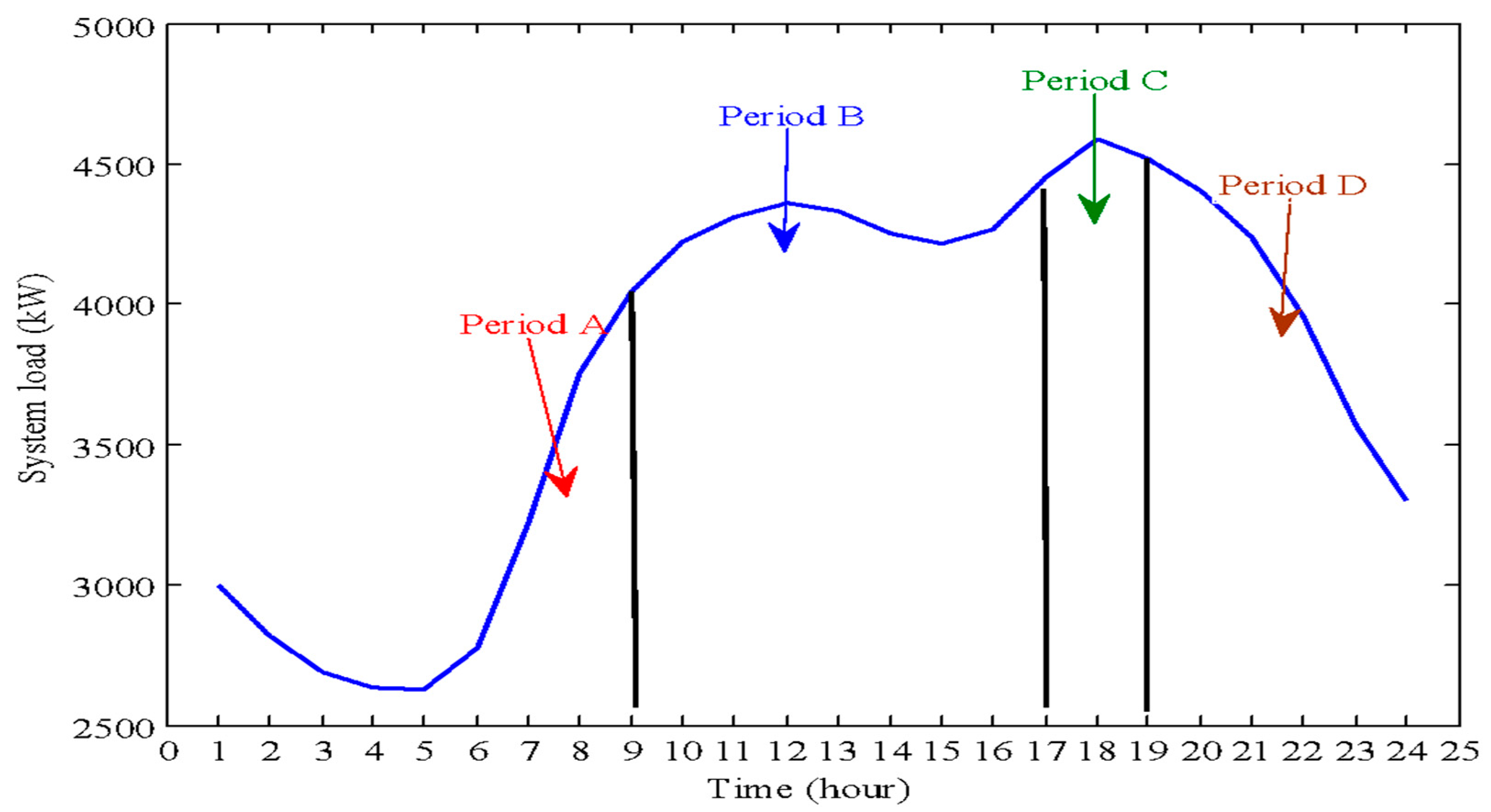
Energies 10 01765 g001
Figure 2. Sectionalized hourly average system load demand profile for 2013.
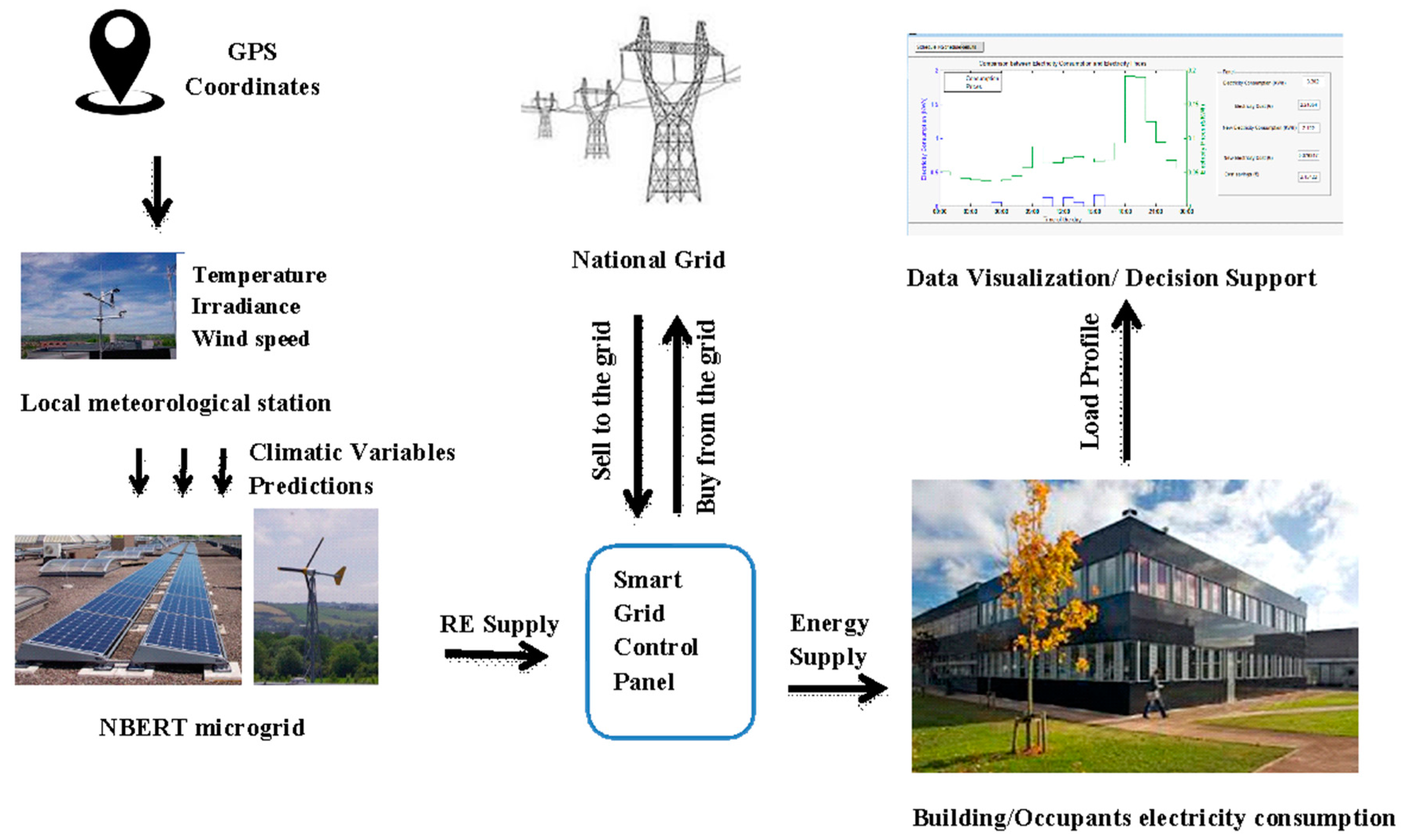
Energies 10 01765 g002
Figure 3. DSTREM system overview.
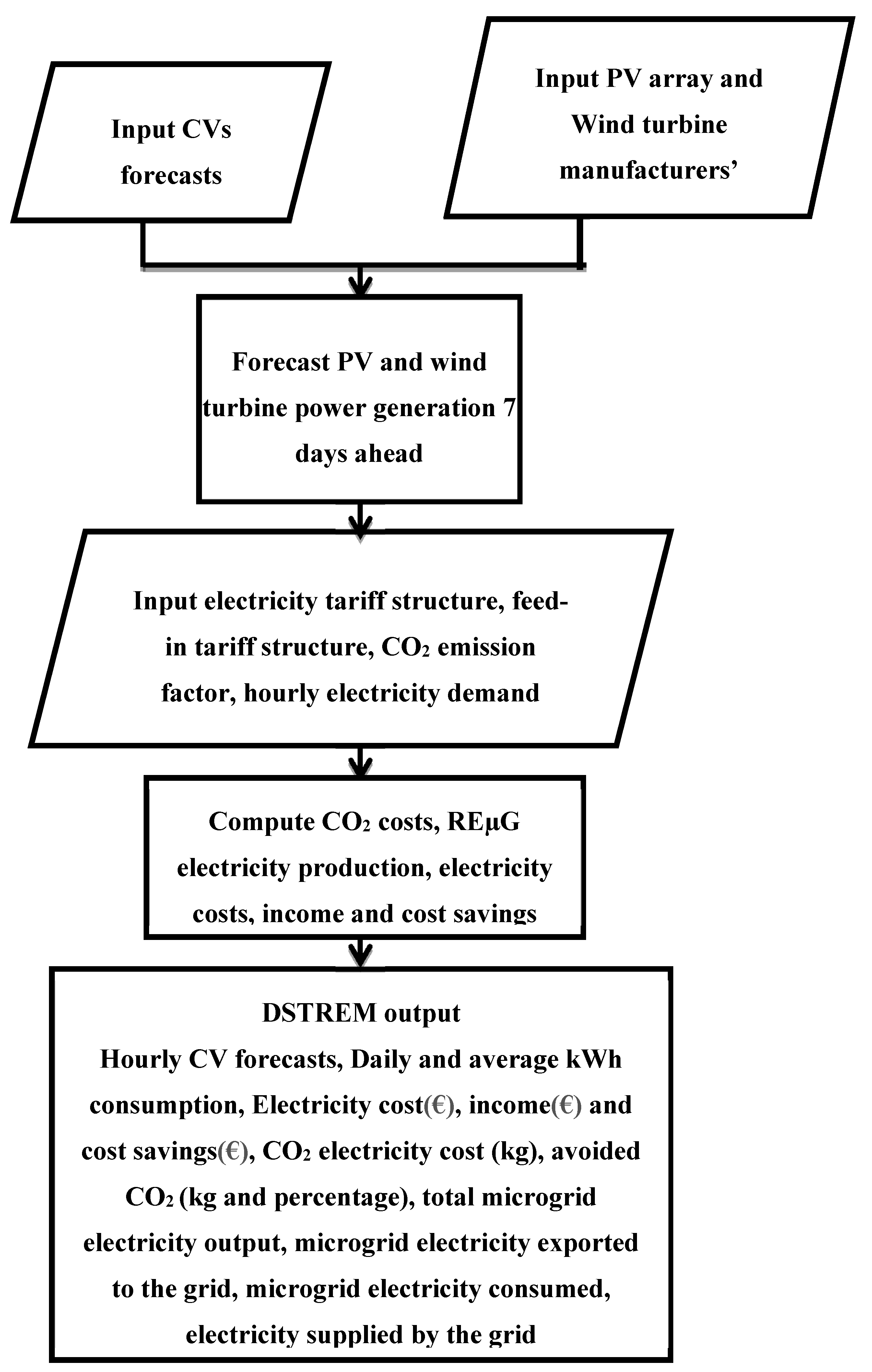
Energies 10 01765 g003
Figure 4. DSTREM process flow chart.
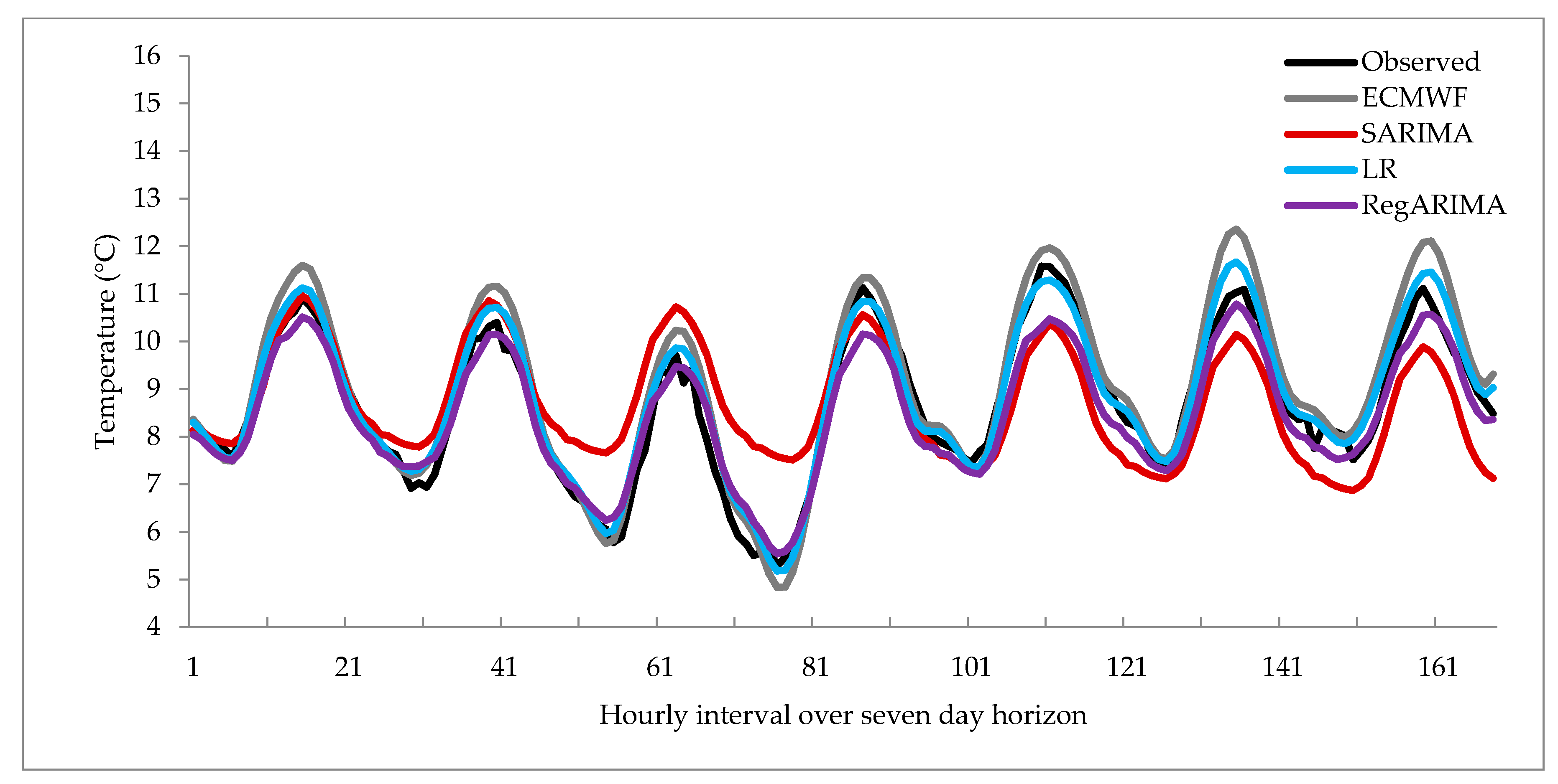
Energies 10 01765 g004
Figure 5. Predicted and observed temperature.
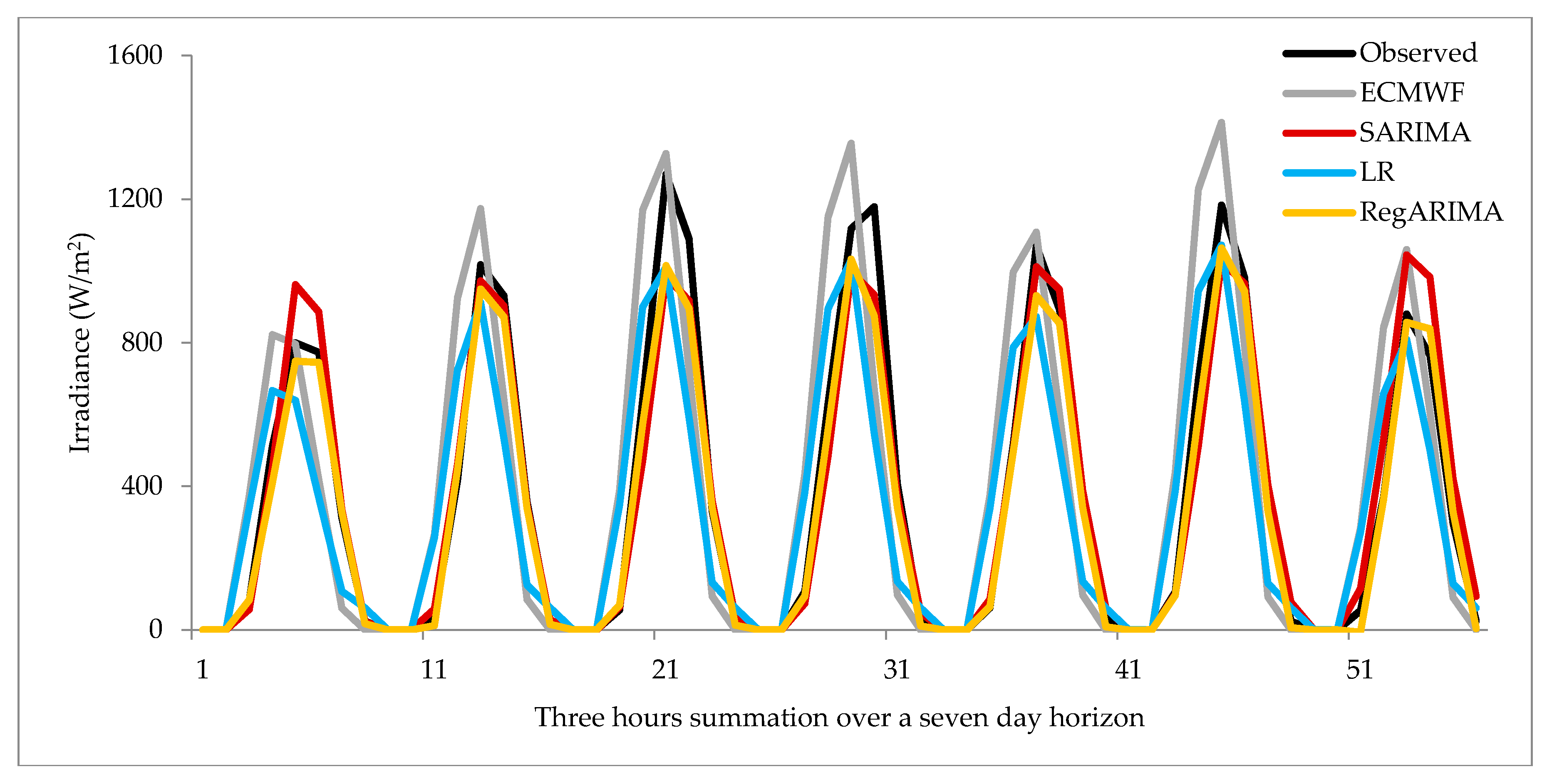
Energies 10 01765 g005
Figure 6. Predicted and observed irradiance.
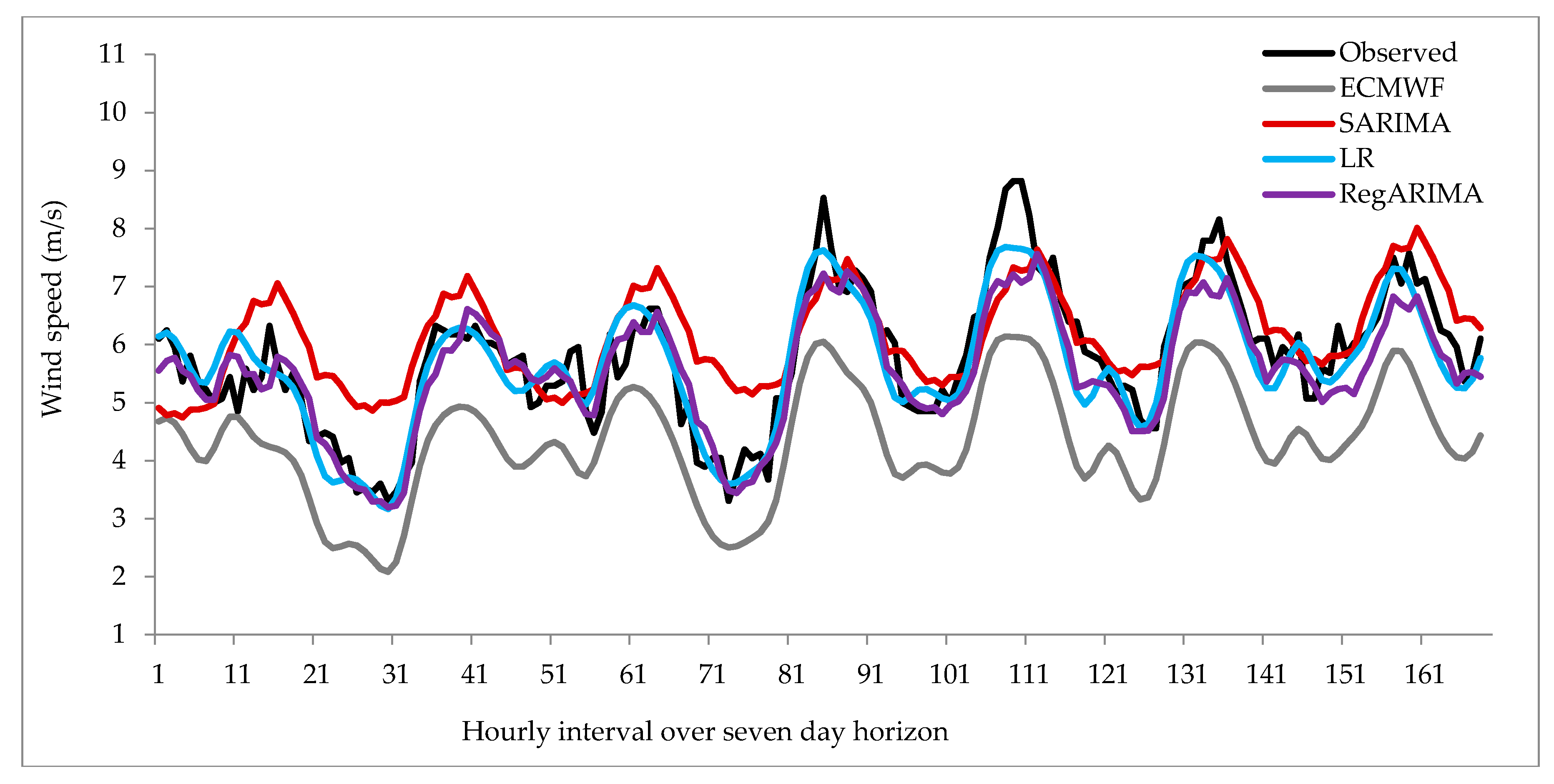
Energies 10 01765 g006
Figure 7. Predicted and observed wind speed.
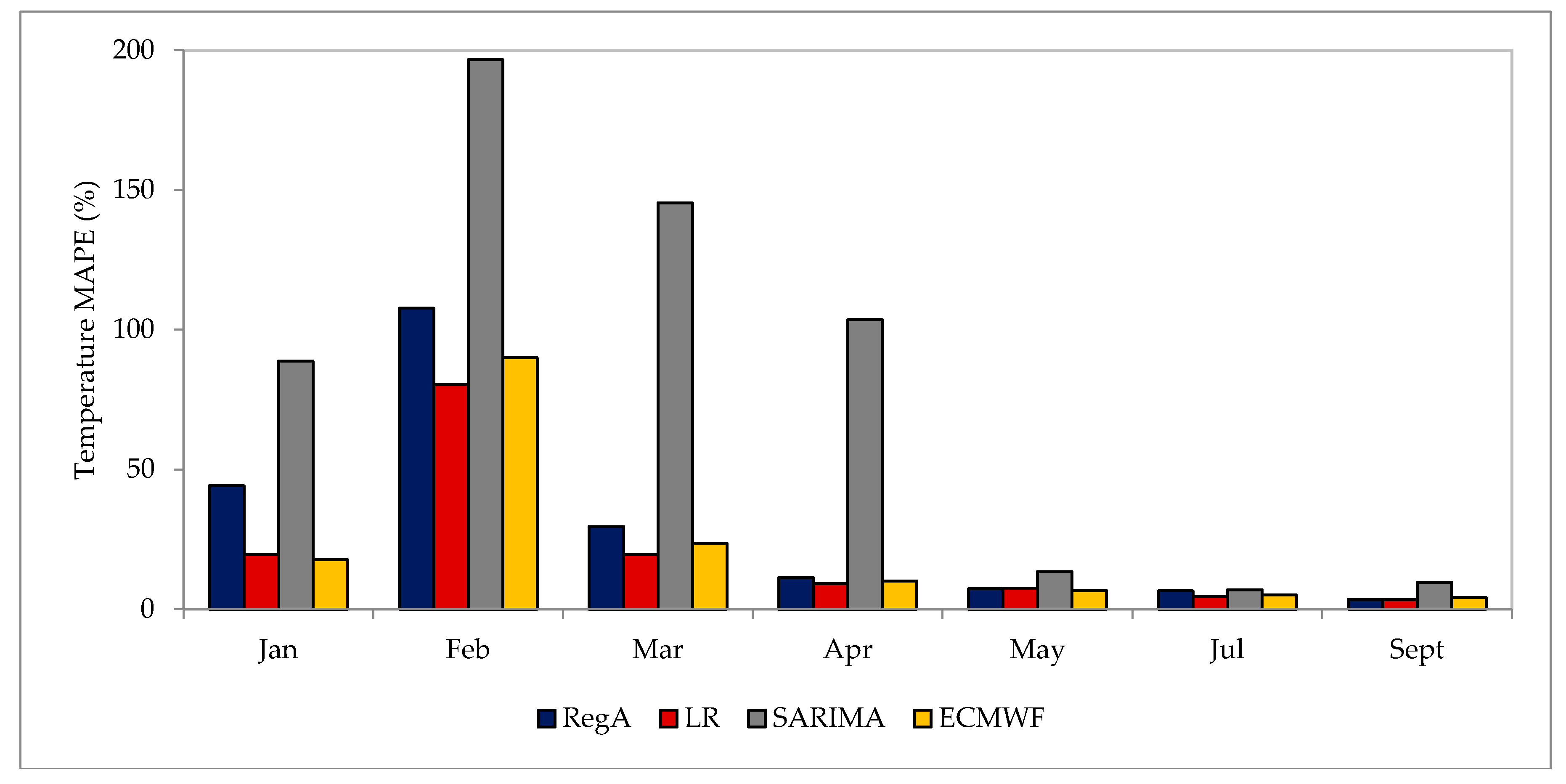
Energies 10 01765 g007
Figure 8. Temperature MAPE for all forecasting models and ECMWF data (RegA denotes RegARIMA model).
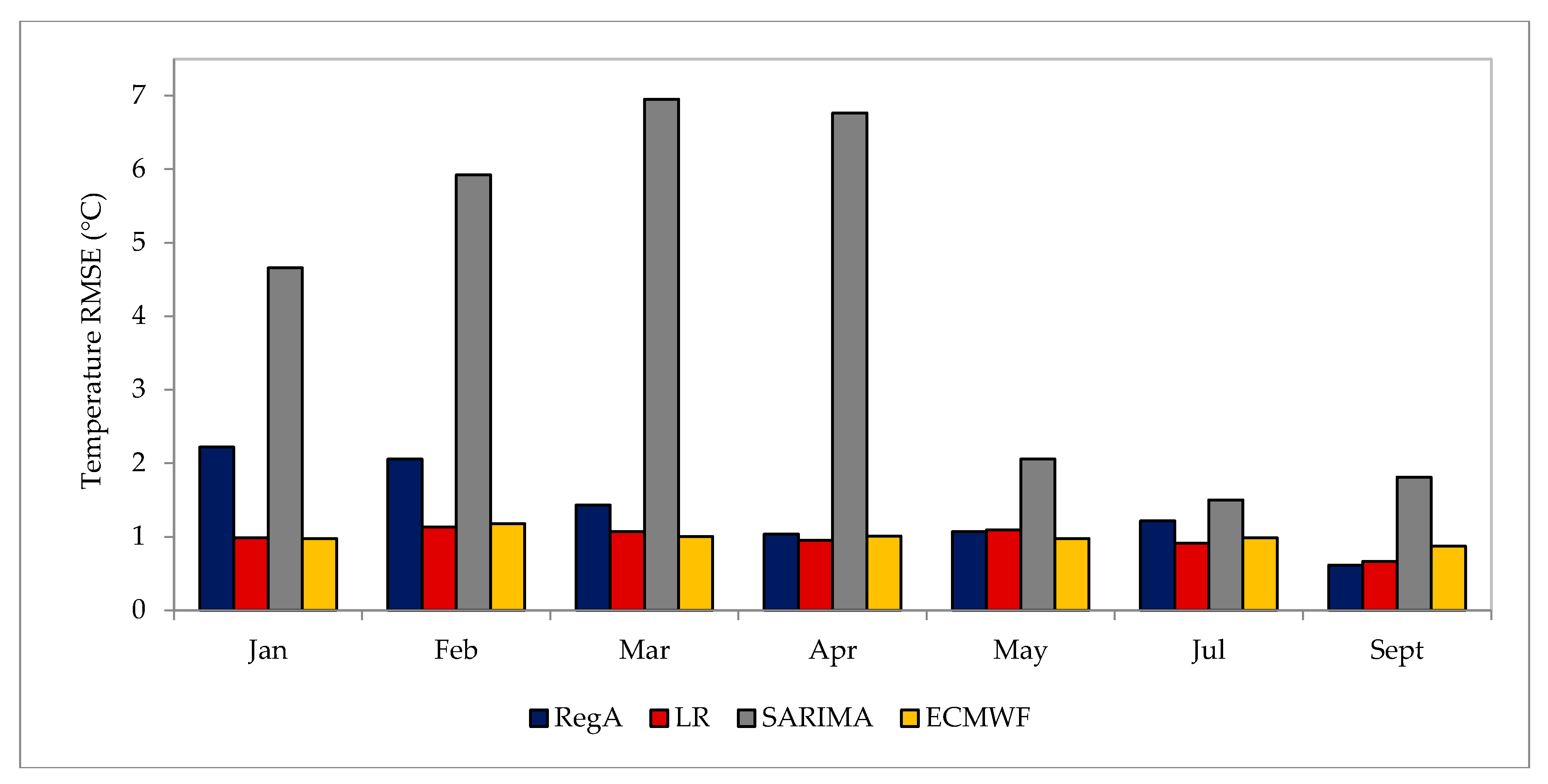
Energies 10 01765 g008
Figure 9. Temperature RMSE for all forecasting models and ECMWF data (RegA denotes RegARIMA model).
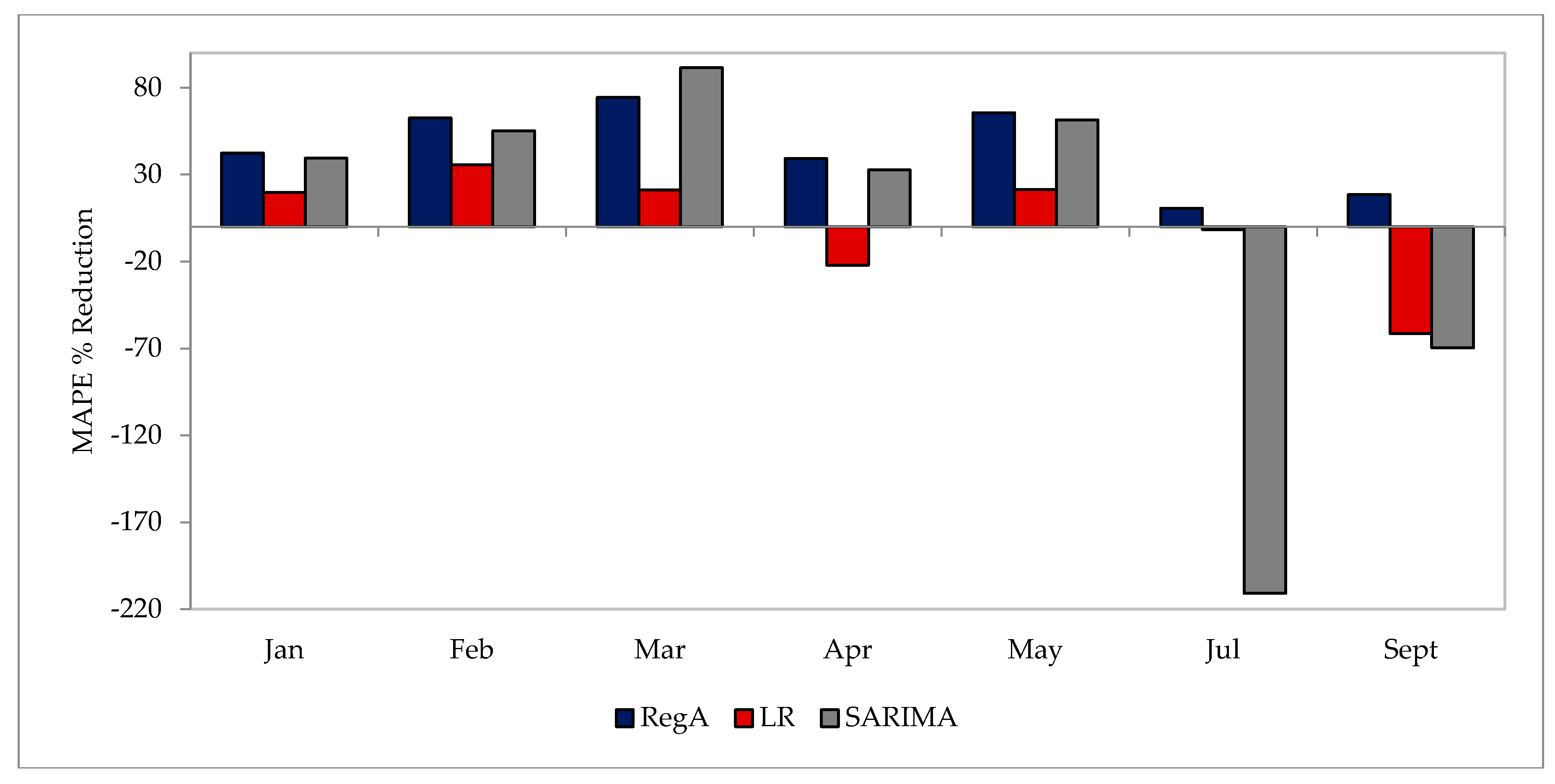
Energies 10 01765 g009
Figure 10. Percentage reduction of temperature MAPE relative to ECMWF data for all forecasting models (RegA denotes RegARIMA model).
Energies 10 01765 g010
Figure 11. Percentage reduction of temperature RMSE relative to ECMWF data for all forecasting models (RegA denotes RegARIMA model).
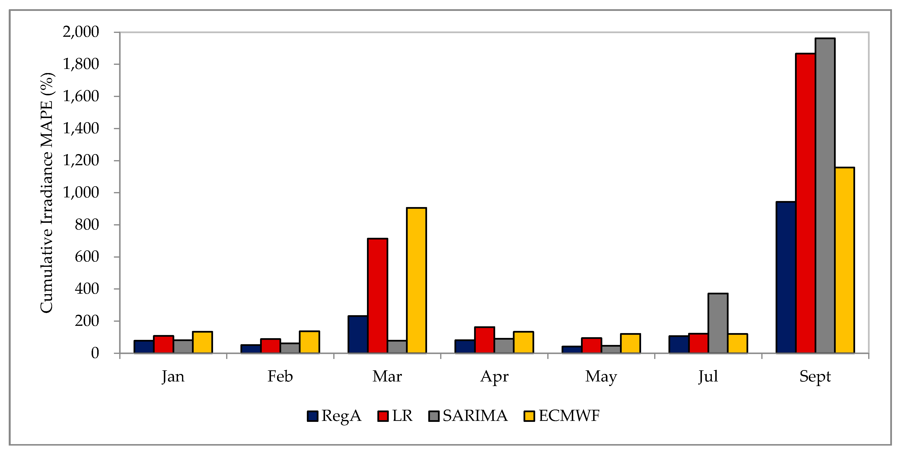
Energies 10 01765 g011
Figure 12. Cumulative irradiance MAPE for all forecasting models and ECMWF data (RegA denotes RegARIMA model).
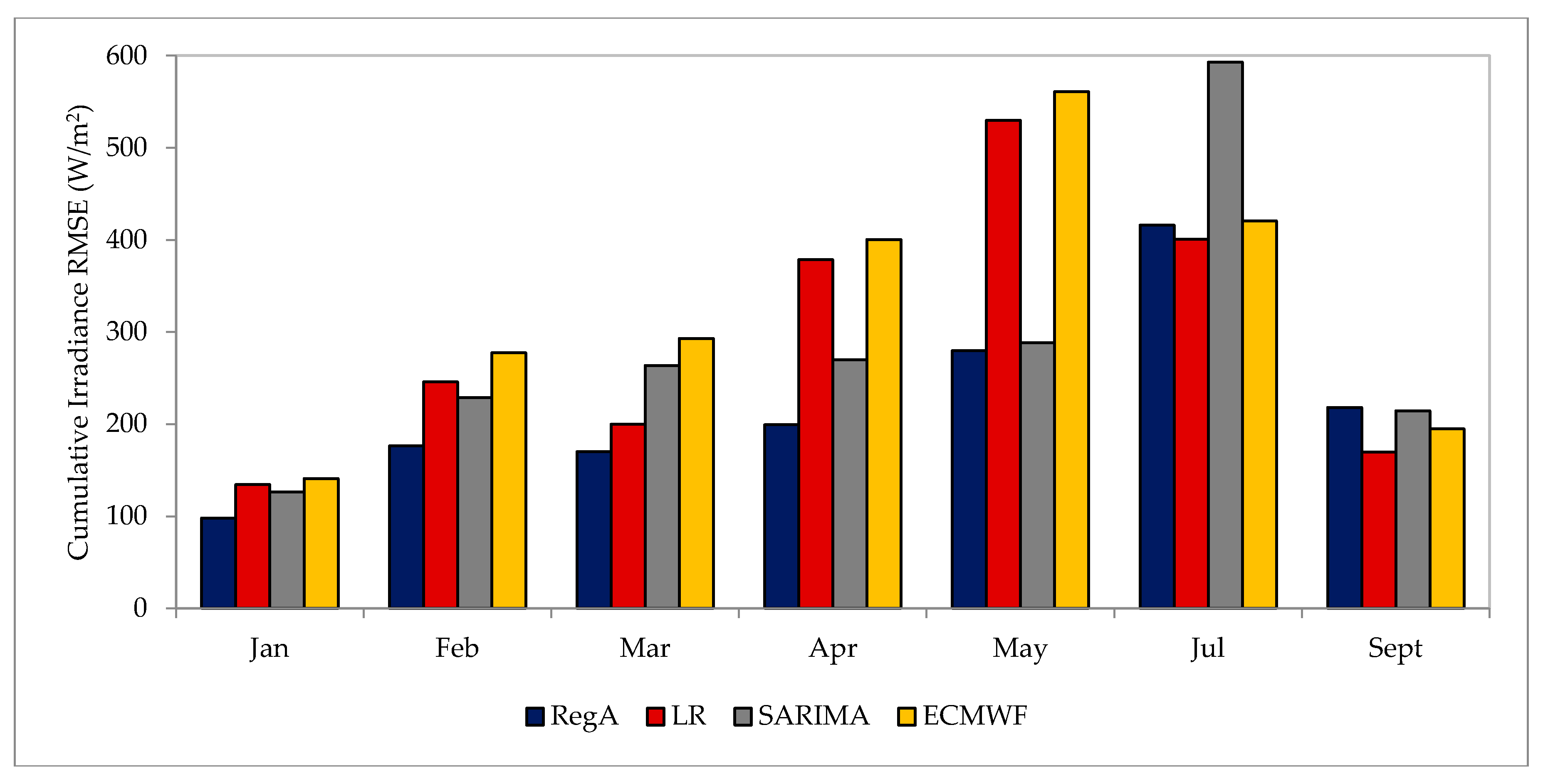
Energies 10 01765 g012
Figure 13. Cumulative irradiance RMSE for all forecasting models and ECMWF data (RegA denotes RegARIMA model).
Energies 10 01765 g013
Figure 14. Percentage reduction of cumulative irradiance MAPE relative to ECMWF data for all forecasting models (RegA denotes RegARIMA model).
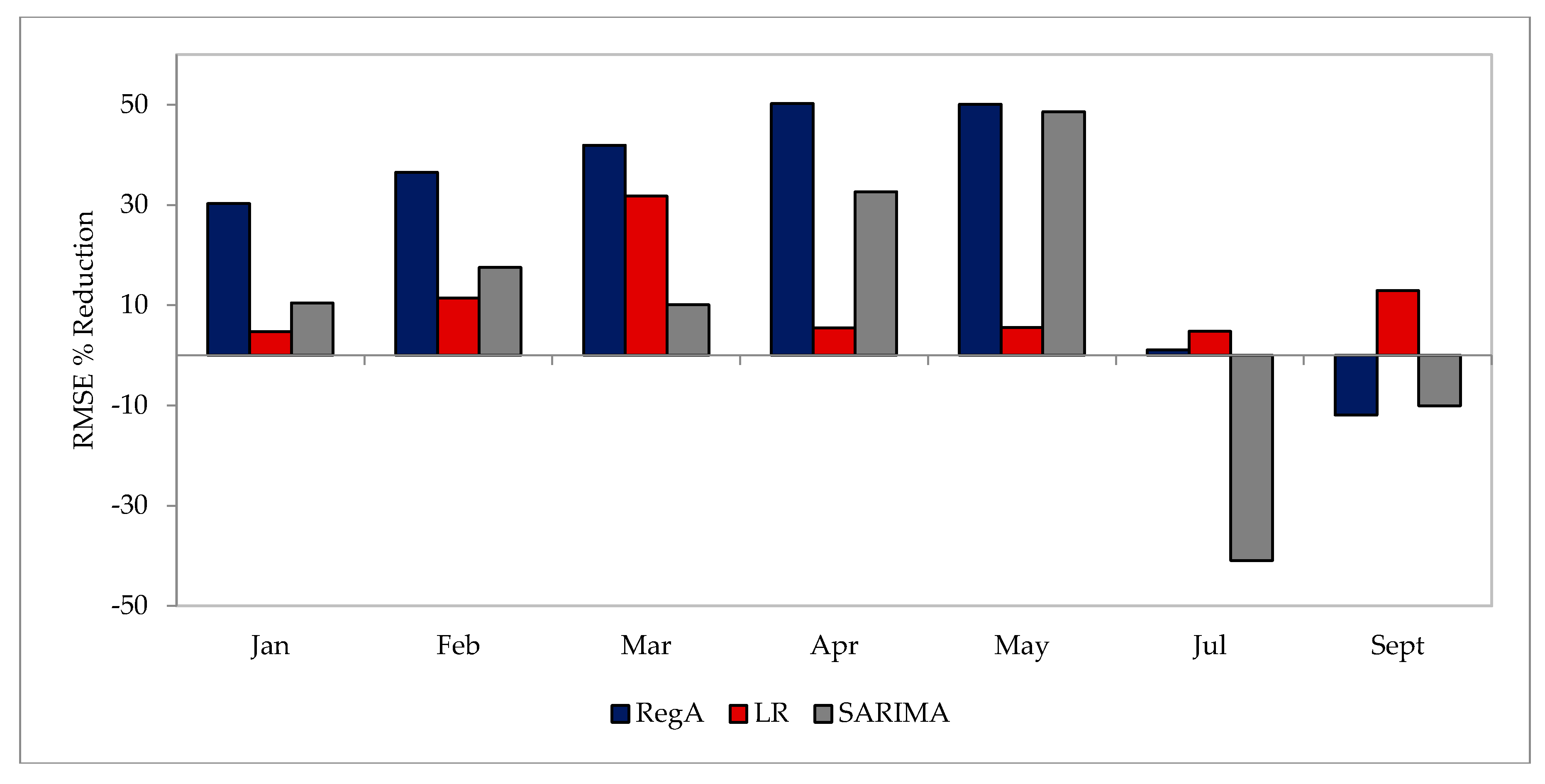
Energies 10 01765 g014
Figure 15. Percentage reduction of cumulative irradiance RMSE relative to ECMWF data for all forecasting models (RegA denotes RegARIMA model).
Energies 10 01765 g015
Figure 16. Wind speed MAPE for all forecasting models and ECMWF data (RegA denotes RegARIMA model).
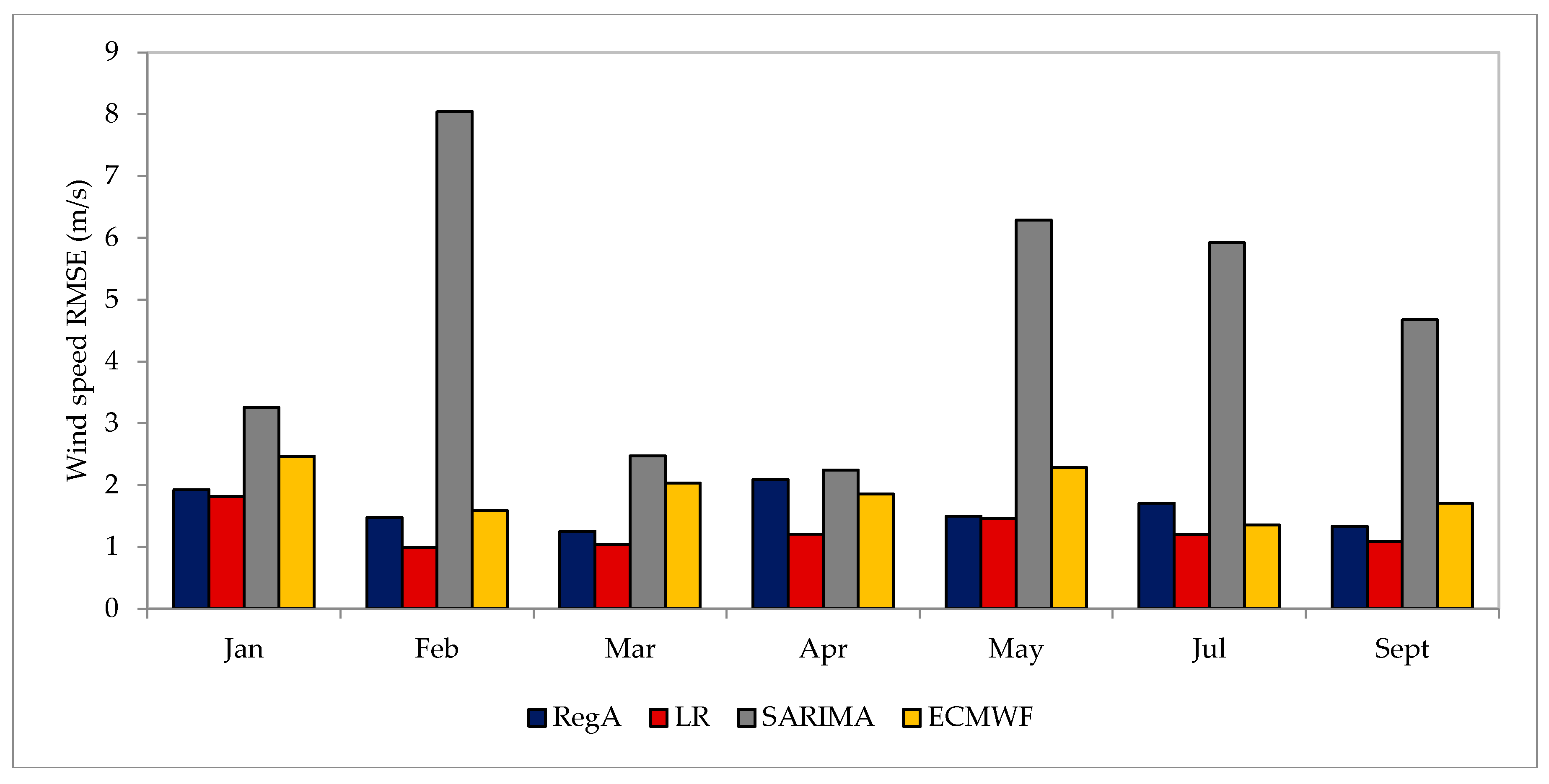
Energies 10 01765 g016
Figure 17. Wind speed RMSE for all forecasting models and ECMWF data (RegA denotes RegARIMA model).
Energies 10 01765 g017
Figure 18. Percentage reduction of wind speed MAPE relative to ECMWF data for all forecasting models (RegA denotes RegARIMA model).
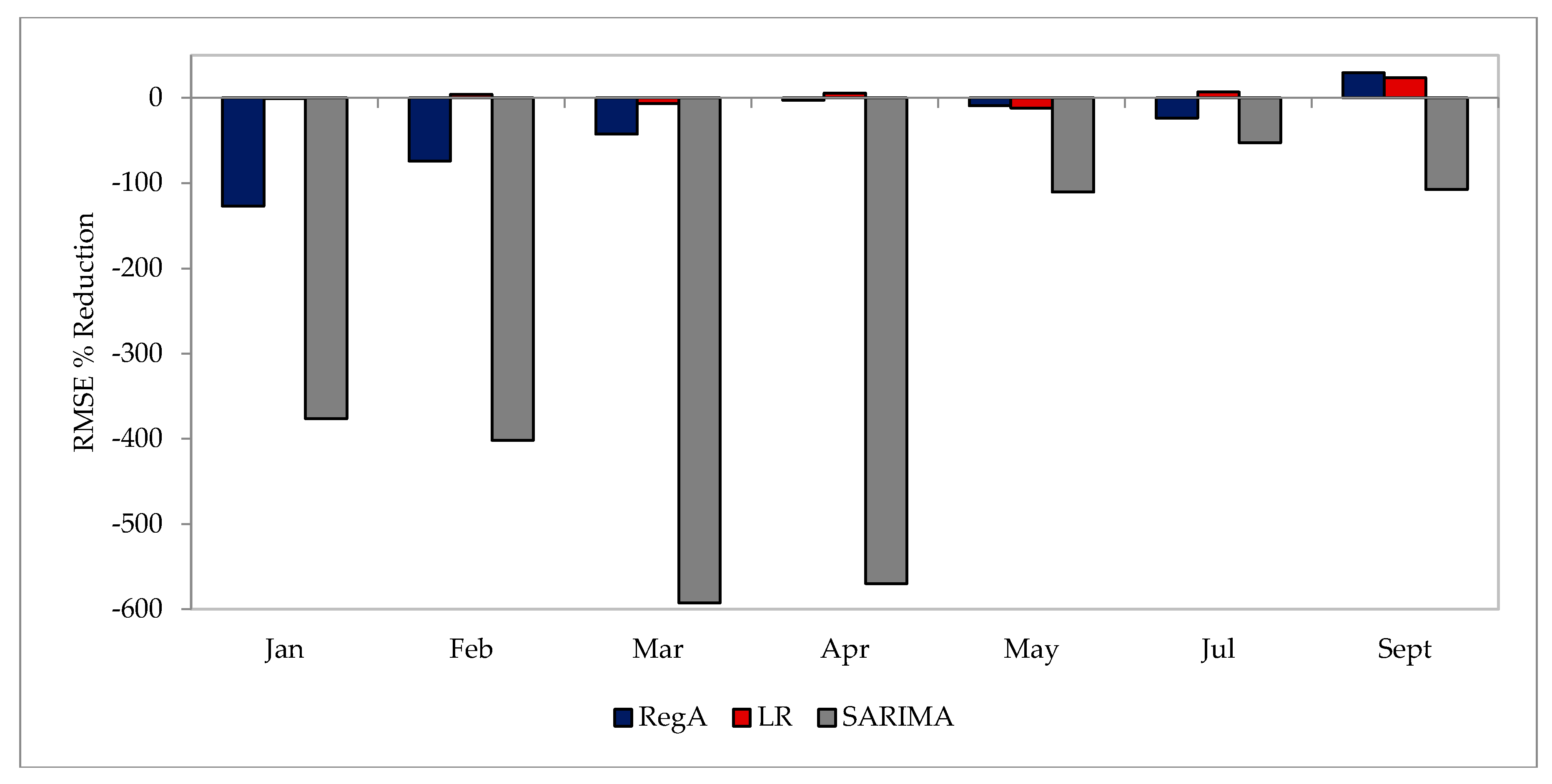
Energies 10 01765 g018
Figure 19. Percentage reduction of wind speed RMSE relative to ECMWF data for all forecasting models (RegA denotes RegARIMA model).
Energies 10 01765 g019
Figure 20. Simulated (using empirical data) and forecasted (using forecasted data) PV array power output (kWh).
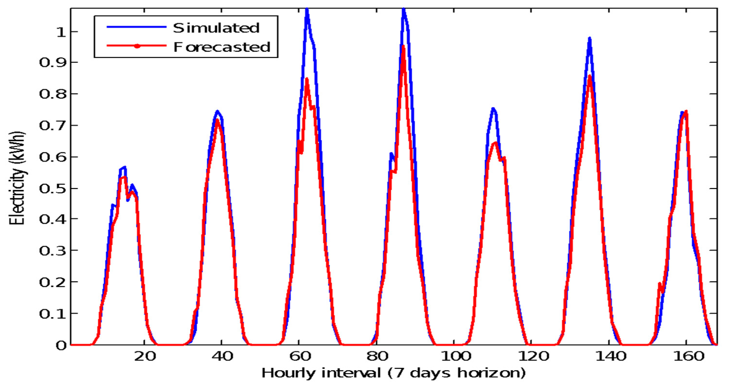
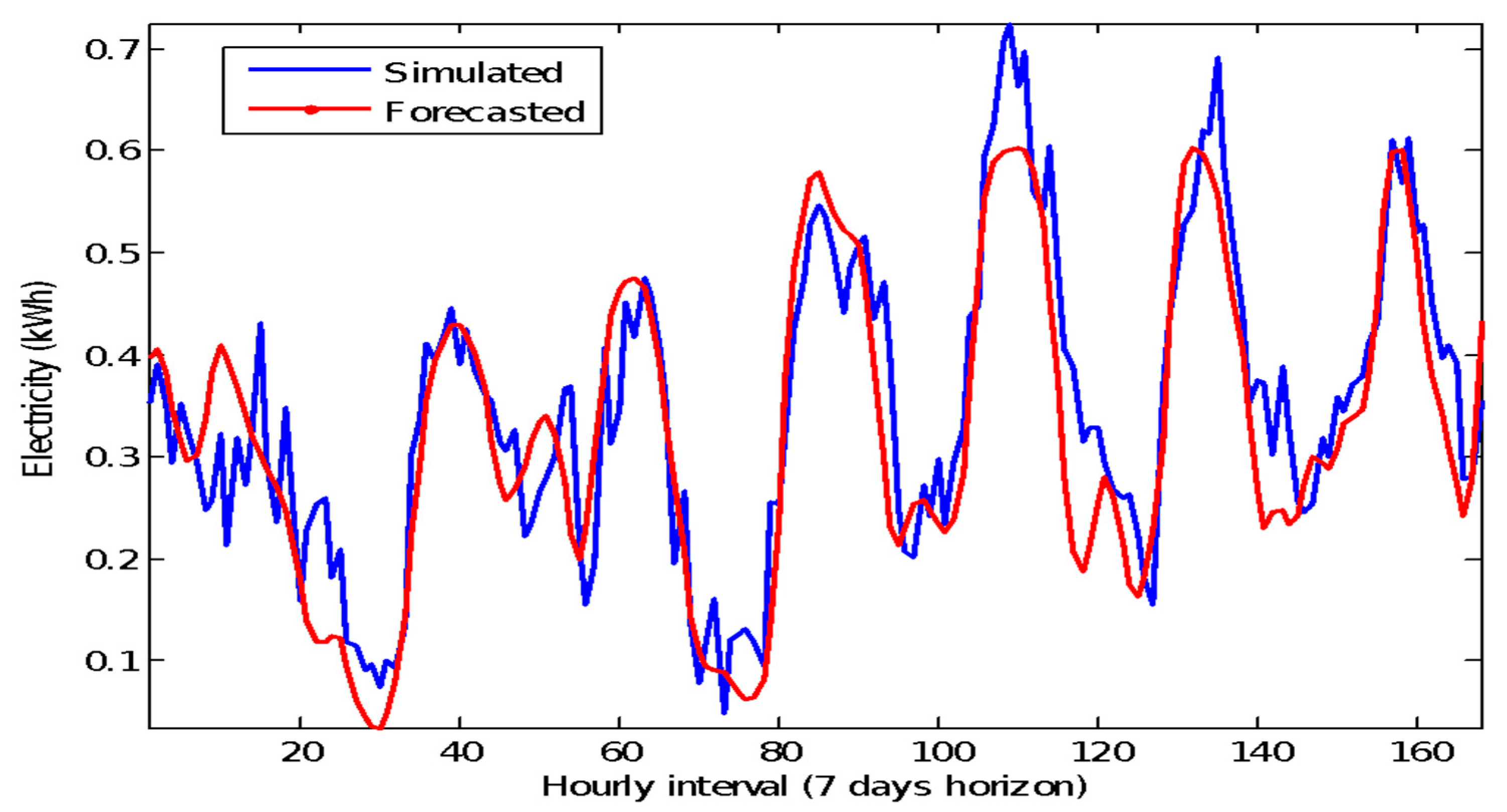
Energies 10 01765 g020
Figure 21. Simulated (using empirical data) and forecasted (using forecasted data) wind turbine power output (kWh).
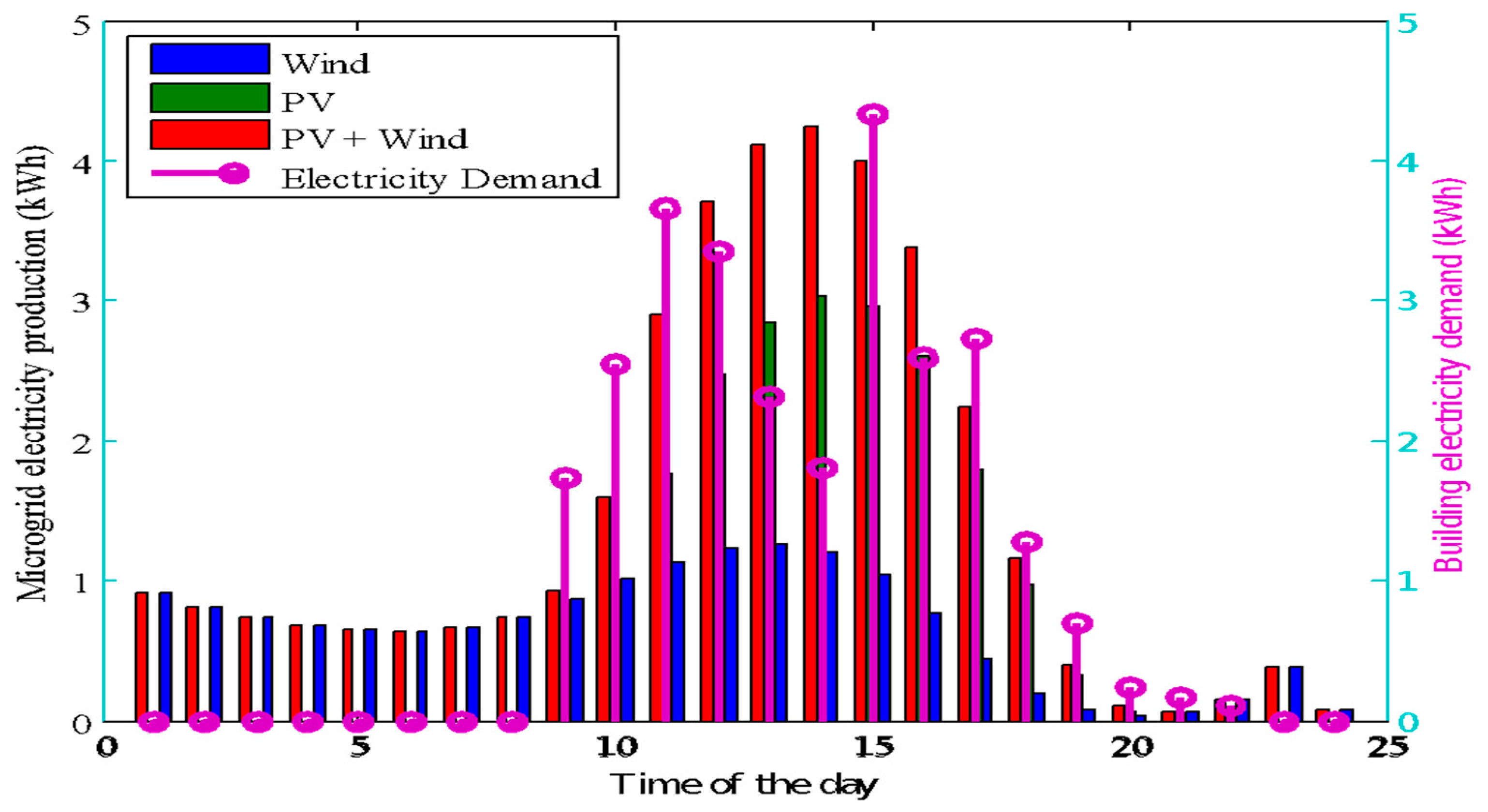
Energies 10 01765 g021
Figure 22. Hourly PV array, wind turbine and PV+Wind turbine power output predictions with corresponding hourly electricity demand totaled across the demonstration week.
Energies 10 01765 g022
Table 1. FIT1 and FIT2 tariff margins for the system demand periods. Percentages shown represent the percentage of the buying price of electricity used to calculate the FIT in each period A to D.
FITPeriod APeriod BPeriod CPeriod D
FIT190%100%110%100%
FIT230%130%200%40%
Table 2. Average RMSE for climatic variable predictions for the year 2013.
Climatic VariableECMWFLRSARIMARegARIMA
Temperature (°C)1.000.974.241.38
Irradiance (W/m2)326.9294.1283.4222.6
Wind Speed (m/s)1.901.264.701.61
Table 3. Average MWE (%) and average MAPE (%) for climatic variable predictions for the year 2013.
Climatic VariableMWE (%)MAPE (%)
ECMWFLRSARIMARegARIMAECMWFLRSARIMARegARIMA
Temperature910−47−1523218130
Irradiance20−1−30387452385219
Wind Speed−117−451−2128229728
Table 4. Average percentage reduction of RMSE and MAPE by LR, SARIMA and RegARIMA relative to ECMWF forecasts.
Climatic VariableRMSE (%)MAPE (%)
LRSARIMARegARIMALRSARIMARegARIMA
Temperature3−316−366−318−32
Irradiance1110282−0.0144
Wind Speed33−1671220−234−0.21
Table 5. Electricity exported (kWh and %), Electricity supplied by REμG (kWh and %), electricity supplied by national smart grid (kWh), percentage RE exported, percentage RE used, avoided CO2 by RE (kg and %) for the three REμG scenarios and for each day of the demonstration week.
DayREµG ScenarioElectricity Export (kWh)Electricity REμG (kWh)Electricity Grid (kWh)% ex% Used% μG% GAvoided CO2 by RE (kg)% Avoided CO2
FridayPV0.011.733.45010033670.7333
Wind6.864.650.53604090102.0390
PV+Wind8.125.130.0561399912.2399
SaturdayPV2.910.000.001000NANANANA
Wind0.160.000.001000NANANANA
PV+Wind3.070.000.001000NANANANA
SundayPV3.170.000.001000NANANANA
Wind0.110.000.001000NANANANA
PV+Wind3.280.000.001000NANANANA
MondayPV0.213.552.3869460401.5259
Wind0.140.455.4723778920.208
PV+Wind0.563.792.13138764361.6363
TuesdayPV0.002.383.62010040601.0239
Wind0.111.005.00109017830.4316
PV+Wind0.313.182.8299153471.3752
WednesdayPV0.021.992.6819943570.8542
Wind0.120.584.09178312880.2512
PV+Wind0.282.422.25109052481.0451
ThursdayPV0.243.282.5179357431.4056
Wind0.491.164.63307020800.5120
PV+Wind0.894.271.51178374261.8473
Table 6. Electricity cost reduction (€ and %) generated by the REμG relative to buying all required electricity from the national smart grid across the three ET structures and the three REμG scenarios for each day of the demonstration week.
DayREµG ScenarioRTP (€)TOU (€)DN (€)RTP (%)TOU (%)DN (%)
FridayPV0.360.270.28343434
Wind0.970.710.72898889
PV+Wind1.070.790.79999999
SaturdayPV0.000.000.00NANANA
Wind0.000.000.00NANANA
PV+Wind0.000.000.00NANANA
SundayPV0.000.000.00NANANA
Wind0.000.000.00NANANA
PV+Wind0.000.000.00NANANA
MondayPV0.750.550.57606062
Wind0.100.070.07888
PV+Wind0.800.580.61646466
TuesdayPV0.500.370.38404041
Wind0.210.150.16171617
PV+Wind0.670.490.51535354
WednesdayPV0.420.320.32434344
Wind0.120.090.09121213
PV+Wind0.510.380.39525253
ThursdayPV0.690.500.52575658
Wind0.240.170.18202020
PV+Wind0.900.650.67747375
Table 7. Daily income (€) and cost savings (€) for three microgrid electricity supply options (PV, Wind, and PV+Wind), under three ET structures (RTP, TOU and DN) for FIT1.
DayIncome (€)Savings (€)
RTPPVWindPV+WindPVWindPV+Wind
Friday0.001.201.460.372.162.53
Saturday0.620.030.650.620.030.65
Sunday0.670.020.690.670.020.69
Monday0.050.020.110.790.120.91
Tuesday0.000.020.060.500.230.73
Wednesday0.000.020.060.420.140.57
Thursday0.050.100.180.740.341.08
TOUPVWindPV+WindPVWindPV+Wind
Friday0.000.891.090.271.601.88
Saturday0.450.020.480.450.020.48
Sunday0.490.010.500.490.010.50
Monday0.030.020.080.580.090.67
Tuesday0.000.020.040.370.170.54
Wednesday0.000.020.040.320.100.42
Thursday0.040.070.130.540.240.78
DNPVWindPV+WindPVWindPV+Wind
Friday0.000.600.800.281.321.60
Saturday0.470.020.490.470.020.49
Sunday0.510.010.520.510.010.52
Monday0.030.010.080.600.080.69
Tuesday0.000.010.040.380.170.55
Wednesday0.000.020.040.320.110.43
Thursday0.040.070.130.560.240.80
Table 8. Daily income (€) and cost savings (€) for three microgrid electricity supply options (PV, Wind, and PV+Wind), under three ET structures (RTP, TOU and DN) for FIT2.
DayIncome (€)Savings(€)
RTPPVWindPV+WindPVWindPV+Wind
Friday0.000.630.980.371.602.05
Saturday0.830.020.840.830.020.84
Sunday0.880.010.890.880.010.89
Monday0.060.010.130.810.100.93
Tuesday0.000.010.060.500.220.73
Wednesday0.000.010.050.420.130.56
Thursday0.070.040.150.760.281.04
TOUPVWindPV+WindPVWindPV+Wind
Friday0.000.460.710.271.171.50
Saturday0.610.010.630.610.010.63
Sunday0.650.010.650.650.010.65
Monday0.050.010.090.590.070.68
Tuesday0.000.010.040.370.160.53
Wednesday0.000.010.040.320.090.42
Thursday0.050.030.110.550.200.76
DNPVWindPV+WindPVWindPV+Wind
Friday0.000.370.640.281.091.43
Saturday0.630.010.640.630.010.64
Sunday0.670.010.680.670.010.68
Monday0.050.000.090.610.080.70
Tuesday0.000.000.040.380.160.55
Wednesday0.000.010.040.320.100.42
Thursday0.050.030.110.570.200.78
Table 9. Daily income (€) and cost savings (€) for three microgrid electricity supply options (PV, Wind, and PV+Wind), under three ET structures (RTP, TOU and DN) for FIT3.
DayIncome (€)Savings (€)
RTPPVWindPV+WindPVWindPV+Wind
Friday0.000.620.730.371.591.80
Saturday0.260.010.280.260.010.28
Sunday0.290.010.300.290.010.30
Monday0.020.010.050.770.110.85
Tuesday0.000.010.030.500.220.70
Wednesday0.000.010.030.420.130.54
Thursday0.020.040.080.710.290.98
TOUPVWindPV+WindPVWindPV+Wind
Friday0.000.620.730.271.331.52
Saturday0.260.010.280.260.010.28
Sunday0.290.010.300.290.010.30
Monday0.020.010.050.570.080.63
Tuesday0.000.010.030.370.160.52
Wednesday0.000.010.030.320.100.41
Thursday0.020.040.080.520.220.73
DNPVWindPV+WindPVWindPV+Wind
Friday0.000.620.730.281.341.52
Saturday0.260.010.280.260.010.28
Sunday0.290.010.300.290.010.30
Monday0.020.010.050.590.080.66
Tuesday0.000.010.030.380.170.53
Wednesday0.000.010.030.320.100.41
Thursday0.020.040.080.540.220.76

