Risk-Based Bi-Level Model for Simultaneous Profit Maximization of a Smart Distribution Company and Electric Vehicle Parking Lot Owner

Abstract

In this paper, the effect of renewable energy resources (RERs), demand response (DR) programs and electric vehicles (EVs) is evaluated on the optimal operation of a smart distribution company (SDISCO) in the form of a new bi-level model. According to the existence of private electric vehicle parking lots (PLs) in the network, the aim of both levels is to maximize the profits of SDISCO and the PL owners. Furthermore, due to the uncertainty of RERs and EVs, the conditional value-at-risk (CVaR) method is applied in order to limit the risk of expected profit. The model is transformed into a linear single-level model by the Karush–Kuhn–Tucker (KKT) conditions and tested on the IEEE 33-bus distribution system over a 24-h period. The results show that by using a proper charging/discharging schedule, as well as a time of use program, SDISCO gains more profit. Furthermore, by increasing the risk aversion parameter, this profit is reduced.

1. Introduction

Nowadays, the planning and operation of the smart distribution company (SDISCO) with the penetration of electric vehicles (EVs) has been complicated due to uncontrolled charging, controlled charging and smart charging/discharging. If uncontrolled charging for the operation of EVs is used, the penetration of EVs yields improper results such as increasing losses [1,2], growing demand [3,4], unbalancing of the load [5,6], voltage drop [7], increasing of total harmonic distortion [8,9], decreasing of cable and transformer life [10,11], etc. However, by using the controlled charging and smart charging/discharging schedule, as well as the vehicle-to-grid (V2G) capability of EVs, the performance of SDISCO is improved. For instance, in [12], by using EVs along with solar panels in a practical form, the peak load is shifted. In [13], the system frequency and continuous supply of demand are controlled in a hybrid power system involving renewable energy resources (RERs), the battery energy storage system and V2G capability. In [14], by modeling the EVs, especially V2G capability and idle mode, a hierarchical coordinated model is designed for the maximization of economic benefit and solving the network unbalancing and congestions. In [15], by proposing a technical and environmental scheduling model of EVs, the operation cost and CO₂ emission are minimized by considering V2G capability.

According to the result of some studies such as [16,17], charging of EVs only with traditional power plants creates some inappropriate environmental impacts. Thus, it is inevitable to use RERs along with these types of power plants. The interactions of EVs with solar photovoltaic (PV) [18,19], wind turbine [20,21] and both [22,23] are investigated.

The demand response (DR) program, which is divided into two groups, i.e., price-based demand response (PBDR) and incentive-based DR (IBDR) program, has become one of the most cost-effective and efficient solutions for reducing the load of SDISCO when the upstream network has a problem with respect to energy generation. For a more accurate assessment of the DR program on SDISCO, a proper model is needed. In [24], the economic model for the time of use (TOU) and emergency DR programs (EDRP) are explained. Moreover, in [25], the modeling of the interruptible/curtailable (I/C) and capacity market programs (CAP) are proposed. In [26], an economic model is obtained for the responsive load based on price elasticity of the demand, electricity price, as well as the incentive and penalty values.

In the most cases, the SDISCO’s purpose is to maximize profits or minimize costs while reducing the associated risk. This risk is because of the existence of uncertainty in the load, electricity price, etc. Usually, risk management is accomplished by means of the so-called risk measures. The profit variance, shortfall probability, expected shortfall, value-at-risk (VaR) and conditional value-at-risk (CVaR) are the examples of risk measures. Recently, for the linear formulation, CVaR has been used widely in the power system problems [27].

In [28], due to market price and load forecast volatilities, for solving the CHP scheduling problem in the presence of DR programs, a CVaR-based stochastic model is presented with the aim of maximizing the profit of the combined heat and power (CHP) owner. In [29], the CVaR-based scheduling model is proposed to maximize the operation revenue for a virtual power plant with the wind unit, PV unit, convention gas turbine, energy storage systems and the IBDR program. In [30], the CVaR-based stochastic scheduling model is suggested for a smart energy hub in the presence of DR programs and the wind unit, for the maximization of profit. In [31], due to the uncertainties in demand and the cost of energy, a CVaR-based model is presented for optimal feeder routing in which the cost of distribution system planning is optimized. In [32], for the siting and sizing of distribution transformers, a CVaR-based model in the low voltage distribution system is proposed. The market price, load growth and failure rate are the uncertainties in [32]. Furthermore, the aim of this model is to minimize the cost of distribution system planning. In [33], a CVaR-based reconfiguration of the active distribution network is presented for loss reduction and reliability improvement, as well as for considering the uncertainty associated with the load, generation and reliability parameter.

If there are two decision makers in the optimization problem in the way that each decision affects the result, a bi-level model can be used. In [34,35], because of the distribution company and microgrid, a bi-level model is suggested. The aim of this model in the upper and lower level is maximizing the profit of the distribution company and minimizing the operation cost of the micro-grid, respectively. This model is converted to a single level by using the Karush–Kuhn–Tucker (KKT) conditions and dual theory. In [36], for maximizing the profit of the active distribution network operator in the upper level and maximizing the social welfare independent system operator (ISO), a stochastic bi-level model is suggested. This model is converted to a mixed integer linear programming (MILP) model by KKT conditions. In [37], according to the commercial virtual power plant and ISO, a three-stage stochastic bi-level model is proposed and converted into an MILP model using KKT conditions and strong duality theory.

In the reviewed references, the operation of SDISCO in the presence of EVs’ parking lots (PLs) and the energy transfer between them have not been addressed. Hence, in this paper, a new bi-level model is presented for the optimal operation of SDISCO due to the fact that PLs can have private owners and the SDISCO operator can own RERs and be responsible for implementing the PBDR and IBDR programs. In this model, at the upper level, the maximization of the profit of SDISCO and at the lower level the maximization of the profit of the PL owner are modeled. Due to the uncertainties in the system and the definition of CVaR, the bi-level model is converted to the risk-based bi-level model. Finally, the model is solved by using the KKT conditions, auxiliary binary variables, sufficiently large constants and stochastic programming.

The main contributions of the paper are as follows:

• Presenting a new risk-based bi-level model with respect to the SDISCO and PL owner and uncertainties.
• Creating a linear single-level model by using KKT conditions and auxiliary binary variables.
• Considering simultaneously RERs and EVs, as well as PBDR and IBDR programs and their uncertainties for the optimal operation of SDISCO.
• Presenting a risk aversion parameter and market price sensitivity analysis of the optimal operation of SDISCO.

The rest of the manuscript is organized as follows. The DR model is explained in Section 2. The formulation of the bi-level model is explained in Section 3. Numerical results are discussed in Section 4. Finally, conclusions are reported in Section 5.

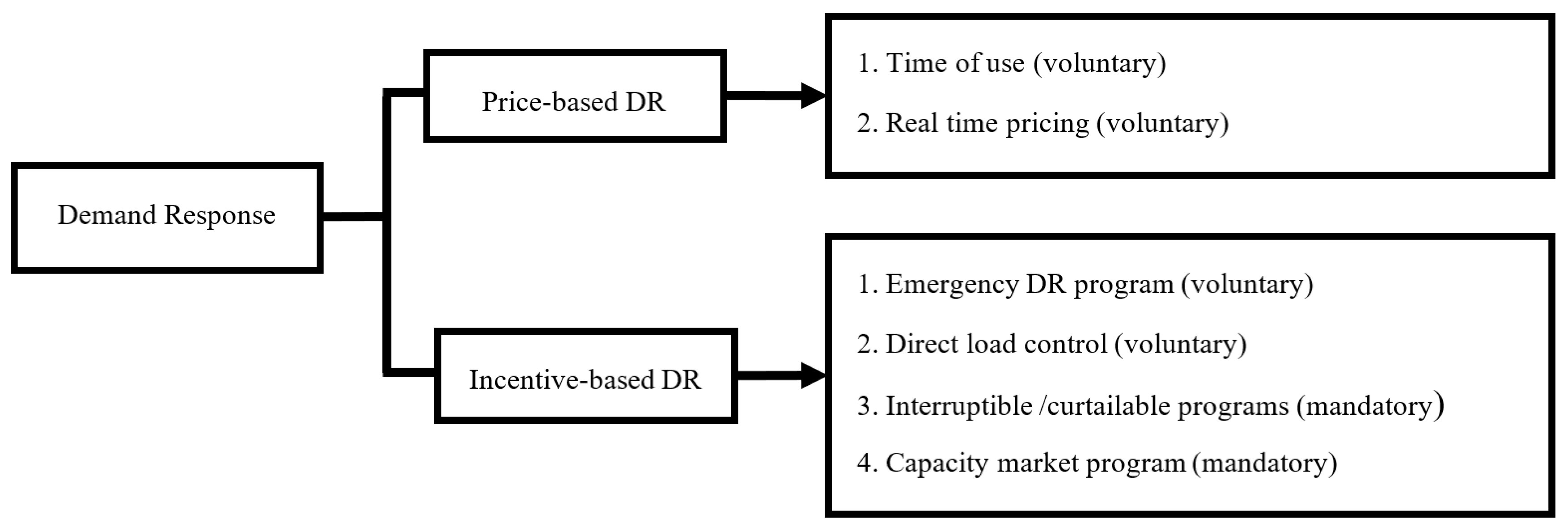
2. Load-Based DR Model

The demand (P) sensitivity with respect to the price (Pr) is defined as elasticity.

$$\mathrm{E}=\frac{\mathrm{P}{\mathrm{r}}_0}{{\mathrm{P}}_0}·\frac{\partial \mathrm{P}}{\partial \mathrm{Pr}}$$

(1)

Based on (1), the load is divided into two types, single-period and multi-period loads. In the first type, known as self-elasticity, the value of elasticity is negative, while in the second type, known as cross-elasticity, the value is positive.

$$\begin{array}{l}\mathrm{E}(\mathrm{t},\mathrm{t})\ge 0\\ E(t,t^{\prime })\ge 0\end{array}$$

(2)

Based on Figure 1, DR programs are divided into two main groups involving PBDR programs and IBDR programs. The PBDR programs are voluntary programs; however, the IBDR programs include voluntary programs, mandatory programs and market clearing programs. Therefore, for the load economic model, we will have [26]:

$$\mathrm{P}(\mathrm{t})={\mathrm{P}}_0(\mathrm{t})\times \left\{1+\mathrm{E}(\mathrm{t},\mathrm{t})\times \frac{\mathrm{Pr}(\mathrm{t})-\mathrm{P}{\mathrm{r}}_0(\mathrm{t})+\mathrm{A}(\mathrm{t})+\mathrm{PEN}(\mathrm{t})}{\mathrm{P}{\mathrm{r}}_0(\mathrm{t})}+{\displaystyle \sum _{{\mathrm{t}}^{\prime }=1,{\mathrm{t}}^{\prime }{}^1\mathrm{t}}^{24}\frac{\mathrm{Pr}({\mathrm{t}}^{\prime })-\mathrm{P}{\mathrm{r}}_0({\mathrm{t}}^{\prime })+\mathrm{A}({\mathrm{t}}^{\prime })+\mathrm{PEN}({\mathrm{t}}^{\prime })}{\mathrm{P}{\mathrm{r}}_0({\mathrm{t}}^{\prime })}\times \mathrm{E}(\mathrm{t},{\mathrm{t}}^{\prime })}\right\}$$

(3)

According to (3), it will be clear how the consumption of customers (P(t)) will change to obtain the maximum profit. The SDISCO is responsible for implementing DR programs. Despite the many benefits of DR, there is an additional cost. This cost (C^DR) is presented in (4).

$${\mathrm{C}}^{\mathrm{D}\mathrm{R}}=\left(\mathrm{A}(\mathrm{t})\times ({\mathrm{P}}_0(\mathrm{t})-\mathrm{P}(\mathrm{t}))\right)-\mathrm{PEN}(\mathrm{t})\times \left({\mathrm{P}}_{\mathrm{con}}(\mathrm{t})-({\mathrm{P}}_0(\mathrm{t})-\mathrm{P}(\mathrm{t}))\right)$$

(4)

3. Problem Formulation

3.1. Bi-Level Model

In this section, a bi-level model is proposed for the operational scheduling. In this model, the main objective of SDISCO is to maximize the profit. This is the upper level problem. Simultaneously, the objective function must also maximize the profits of the PL owner, which is the lower level problem. The proposed upper level, including the objective function and constraints, is formulated in (5)–(21). The objective function of this level is:

$$Objectivefunction={\displaystyle \sum _{\mathrm{s}=1}^{\mathrm{Ns}}{\mathsf{\rho }}_{\mathrm{s}}}\left(\begin{array}{l}{\displaystyle \sum _{\mathrm{n}=1}^{\mathrm{N}}{\displaystyle \sum _{\mathrm{t}=1}^{24}{\mathrm{P}}_{\mathrm{n},\mathrm{t},\mathrm{s}}^{\mathrm{ch}}\times \mathrm{P}{\mathrm{r}}_{\mathrm{t}}^{\mathrm{G}2\mathrm{PL}}}}+{\displaystyle \sum _{\mathrm{b}=2}^{\mathrm{Nb}}{\displaystyle \sum _{\mathrm{t}=1}^{24}{\mathrm{P}}_{\mathrm{b},\mathrm{t},\mathrm{s}}^{\mathrm{L},\mathrm{DR}}\times \mathrm{P}{\mathrm{r}}_{\mathrm{t}}^{\mathrm{G}2\mathrm{L},\mathrm{DR}}}}-{\displaystyle \sum _{\mathrm{Sb}=1}^{\mathrm{NSb}}{\displaystyle \sum _{\mathrm{t}=1}^{24}{\mathrm{P}}_{\mathrm{Sb},\mathrm{t},\mathrm{s}}^{\mathrm{Wh}2\mathrm{G}}\times \mathrm{P}{\mathrm{r}}_{\mathrm{t}}^{\mathrm{Wh}2\mathrm{G}}}}\\ -{\displaystyle \sum _{\mathrm{n}=1}^{\mathrm{N}}{\displaystyle \sum _{\mathrm{t}=1}^{24}{\mathrm{P}}_{\mathrm{n},\mathrm{t},\mathrm{s}}^{\mathrm{dcn}}\times \mathrm{P}{\mathrm{r}}_{\mathrm{t}}^{\mathrm{PL}2\mathrm{G}}}}-{\displaystyle \sum _{\mathrm{b}=2}^{\mathrm{Nb}}{\displaystyle \sum _{\mathrm{t}=1}^{24}\left({\mathrm{A}}_{\mathrm{t}}\left({\mathrm{P}}_{\mathrm{b},\mathrm{t},\mathrm{s}}^{\mathrm{L}}-{\mathrm{P}}_{\mathrm{b},\mathrm{t},\mathrm{s}}^{\mathrm{L},\mathrm{DR}}\right)-{\mathrm{PEN}}_t\left({\mathrm{P}}_{\mathrm{b},\mathrm{t},\mathrm{s}}^{\mathrm{con}}-{\mathrm{P}}_{\mathrm{b},\mathrm{t},\mathrm{s}}^{\mathrm{L}}+{\mathrm{P}}_{\mathrm{b},\mathrm{t},\mathrm{s}}^{\mathrm{L},\mathrm{DR}}\right)\right)}}\end{array}\right)$$

(5)

The important terms in Objective (5) are the revenue from the selling of energy to PL and load (first and second terms), the cost of providing power from the wholesale market (third term), the cost of energy purchased from PL (fourth term) and the cost of the implementation of the PBDR and IBDR programs. In the above equation, P^ch and P^dch are the power that the PL purchased from SDISCO for EVs’ charging and the power that PL sold to SDISCO due to the discharging of EVs, respectively. The customers’ demand after and before DR programs is described by P^{L, DR} and P^L, respectively. P^Wh2G denotes the power purchased from the wholesale market by SDISCO for supplying the PL and customers. It is noted that the part of the customers’ demand (P^{L, DR} or P^L) is provided by the wind and solar units (for which the SDISCO is their owner), partly by power discharging of EVs (P^dch) and partly from the wholesale market (P^Wh2G). Furthermore, P^con is the contracted power in DR programs. The electricity price of power purchased from SDISCO by PL and the electricity price of customer demand after DR are represented by Pr^G2PL and Pr^{G2L, DR}, respectively. Moreover, Pr^PL2G denotes the electricity price of the power that the PL sold to SDISCO. Pr^Wh2G represents the electricity price of the power purchased from the wholesale market.

Moreover, the constraints are limited to the objective function. The importance of these constraints is wind and PV generation, line current, bus voltage and power balance. These constraints are expressed in (6)–(10), respectively. It is noted that for the power flow, in this paper, a linear power flow is used based on (11)–(21) [38].

$$0\le P_{b,t,s}^W\le {\mathrm{P}}^{\mathrm{W},\max }$$

(6)

$$0\le P_{b,t,s}^{PV}\le {\mathrm{P}}^{\mathrm{PV},\max }$$

(7)

$$I_{\mathrm{b},\mathrm{t},\mathrm{s}}\le {\mathrm{I}}_{\mathrm{b}}^{\max }$$

(8)

$${\mathrm{V}}_{\min }=0.95\le V_{\mathrm{b},\mathrm{t},\mathrm{s}}\le {\mathrm{V}}_{\max }=1.05$$

(9)

$$P_{\mathrm{Sb},\mathrm{t},\mathrm{s}}^{\mathrm{Wh}2\mathrm{G}}+P_{b,t,s}^W+P_{b,t,s}^{PV}+{\displaystyle \sum _{\mathrm{N}}{P}_{\mathrm{n},\mathrm{t},\mathrm{s}}^{\mathrm{dch}}}={\mathrm{P}}_{\mathrm{b},\mathrm{t},\mathrm{s}}^{\mathrm{L},\mathrm{DR}}+P_{\mathrm{t},\mathrm{s}}^{\mathrm{Loss}}+{\displaystyle \sum _{\mathrm{N}}{P}_{\mathrm{n},\mathrm{t},\mathrm{s}}^{\mathrm{ch}}}$$

(10)

$$P_{\mathrm{Sb},\mathrm{t},\mathrm{s}}^{\mathrm{Wh}2\mathrm{G}}+P_{b,t,s}^{PV}+P_{b,t,s}^W+{\displaystyle \sum _{\mathrm{N}}{P}_{\mathrm{n},\mathrm{t},\mathrm{s}}^{\mathrm{dch}}-}{\displaystyle \sum _{\mathrm{N}}{P}_{\mathrm{n},\mathrm{t},\mathrm{s}}^{\mathrm{ch}}+{\displaystyle \sum _{b^{\prime }}\left(P_{{\mathrm{b}}^{\prime },\mathrm{b},\mathrm{t},\mathrm{s}}^{+}-P_{{\mathrm{b}}^{\prime },\mathrm{b},\mathrm{t},\mathrm{s}}^{-}\right)}-{\mathrm{P}}_{\mathrm{b},\mathrm{t},\mathrm{s}}^{\mathrm{L},\mathrm{DR}}}-{\displaystyle \sum _{b^{\prime }}\left[\left(P_{\mathrm{b},{\mathrm{b}}^{\prime },\mathrm{t},\mathrm{s}}^{+}-P_{\mathrm{b},{\mathrm{b}}^{\prime },\mathrm{t},\mathrm{s}}^{-}\right)+{\mathrm{R}}_{\mathrm{b},{\mathrm{b}}^{\prime }}I{2}_{\mathrm{b},{\mathrm{b}}^{\prime },\mathrm{t},\mathrm{s}}\right]}=0$$

(11)

$$Q_{\mathrm{Sb},\mathrm{t},\mathrm{s}}^{\mathrm{Wh}2\mathrm{G}}+{\displaystyle \sum _{b^{\prime }}\left(Q_{{\mathrm{b}}^{\prime },\mathrm{b},\mathrm{t},\mathrm{s}}^{+}-Q_{{\mathrm{b}}^{\prime },\mathrm{b},\mathrm{t},\mathrm{s}}^{-}\right)}-{\mathrm{Q}}_{\mathrm{b},\mathrm{t},\mathrm{s}}^{\mathrm{L},\mathrm{DR}}-{\displaystyle \sum _{b^{\prime }}\left[(Q_{\mathrm{b},{\mathrm{b}}^{\prime },\mathrm{t},\mathrm{s}}^{+}-Q_{\mathrm{b},{\mathrm{b}}^{\prime },\mathrm{t},\mathrm{s}}^{-})+{\mathrm{X}}_{\mathrm{b},{\mathrm{b}}^{\prime }}I{2}_{\mathrm{b},{\mathrm{b}}^{\prime },\mathrm{t},\mathrm{s}}\right]}=0$$

(12)

$$0\le \left(P_{\mathrm{b},{\mathrm{b}}^{\prime },\mathrm{t},\mathrm{s}}^{+}+P_{\mathrm{b},{\mathrm{b}}^{\prime },\mathrm{t},\mathrm{s}}^{-}\right)\le {\mathrm{V}}_{\mathrm{Rated}}\times {\mathrm{I}}_{\max ,\mathrm{b},{\mathrm{b}}^{\prime }}$$

(13)

$$0\le \left(Q_{\mathrm{b},{\mathrm{b}}^{\prime },\mathrm{t},\mathrm{s}}^{+}+Q_{\mathrm{b},{\mathrm{b}}^{\prime },\mathrm{t},\mathrm{s}}^{-}\right)\le {\mathrm{V}}_{\mathrm{Rated}}\times {\mathrm{I}}_{\max ,\mathrm{b},{\mathrm{b}}^{\prime }}$$

(14)

$$V{2}_{\mathrm{b},\mathrm{t},\mathrm{s}}-V{2}_{{\mathrm{b}}^{\prime },\mathrm{t},\mathrm{s}}-{\mathrm{Z}}_{\mathrm{b},{\mathrm{b}}^{\prime }}^{2}I{2}_{\mathrm{b},{\mathrm{b}}^{\prime },\mathrm{t},\mathrm{s}}-2{\mathrm{R}}_{\mathrm{b},{\mathrm{b}}^{\prime }}(P_{\mathrm{b},{\mathrm{b}}^{\prime },\mathrm{t},\mathrm{s}}^{+}-P_{\mathrm{b},{\mathrm{b}}^{\prime },\mathrm{t},\mathrm{s}}^{-})-2{\mathrm{X}}_{\mathrm{b},{\mathrm{b}}^{\prime }}(Q_{\mathrm{b},{\mathrm{b}}^{\prime },\mathrm{t},\mathrm{s}}^{+}-Q_{\mathrm{b},{\mathrm{b}}^{\prime },\mathrm{t},\mathrm{s}}^{-})=0$$

(15)

$$\mathrm{V}{2}_{\mathrm{Rated},\mathrm{b}}I{2}_{\mathrm{b},{\mathrm{b}}^{\prime },\mathrm{t},\mathrm{s}}={\displaystyle \sum _{\mathrm{f}}\left[(2f-1)\Delta {\mathrm{S}}_{\mathrm{b},{\mathrm{b}}^{\prime }}\Delta P_{\mathrm{b},{\mathrm{b}}^{\prime },\mathrm{f},\mathrm{t},\mathrm{s}}\right]}+{\displaystyle \sum _{\mathrm{f}}\left[(2f-1)\Delta {\mathrm{S}}_{\mathrm{b},{\mathrm{b}}^{\prime }}\Delta Q_{\mathrm{b},{\mathrm{b}}^{\prime },\mathrm{f},\mathrm{t},\mathrm{s}}\right]}$$

(16)

$$P_{\mathrm{b},{\mathrm{b}}^{\prime },\mathrm{t},\mathrm{s}}^{+}+P_{\mathrm{b},{\mathrm{b}}^{\prime },\mathrm{t},\mathrm{s}}^{-}={\displaystyle \sum _f\Delta P_{\mathrm{b},{\mathrm{b}}^{\prime },\mathrm{f},\mathrm{t},\mathrm{s}}}$$

(17)

$$Q_{\mathrm{b},{\mathrm{b}}^{\prime },\mathrm{t},\mathrm{s}}^{+}+Q_{\mathrm{b},{\mathrm{b}}^{\prime },\mathrm{t},\mathrm{s}}^{-}={\displaystyle \sum _f\Delta Q_{\mathrm{b},{\mathrm{b}}^{\prime },\mathrm{f},\mathrm{t},\mathrm{s}}}$$

(18)

$$0\le \Delta P_{\mathrm{b},{\mathrm{b}}^{\prime },\mathrm{f},\mathrm{t},\mathrm{s}}\le \Delta {\mathrm{S}}_{\mathrm{b},{\mathrm{b}}^{\prime }}$$

(19)

$$0\le \Delta Q_{\mathrm{b},{\mathrm{b}}^{\prime },\mathrm{f},\mathrm{t},\mathrm{s}}\le \Delta {\mathrm{S}}_{\mathrm{b},{\mathrm{b}}^{\prime }}$$

(20)

$$\Delta {\mathrm{S}}_{\mathrm{b},{\mathrm{b}}^{\prime }}=\frac{{\mathrm{V}}_{\mathrm{Rated}}\times I_{\max ,\mathrm{b},{\mathrm{b}}^{\prime }}}{\mathrm{F}}$$

(21)

The lower level problem is to maximize the profit of the PL owner and can be defined as in (22), subject to the constraints in (23)–(27).

$$Objectivefunction={\displaystyle \sum _{\mathrm{s}=1}^{\mathrm{Ns}}{\mathsf{\rho }}_{\mathrm{s}}}\left(\begin{array}{l}{\displaystyle \sum _{\mathrm{n}=1}^{\mathrm{N}}{\displaystyle \sum _{\mathrm{t}=1}^{24}{P}_{\mathrm{n},\mathrm{t},\mathrm{s}}^{ch}\times }}\mathrm{P}{\mathrm{r}}_{\mathrm{t}}^{\mathrm{PL}2\mathrm{EV}}+{\displaystyle \sum _{n=1}^{\mathrm{N}}{\displaystyle \sum _{t=1}^{24}{P}_{\mathrm{n},\mathrm{t},\mathrm{s}}^{dch}\times \mathrm{P}{\mathrm{r}}_{\mathrm{t}}^{\mathrm{PL}2\mathrm{G}}}}-{\displaystyle \sum _{\mathrm{n}=1}^{\mathrm{N}}{\displaystyle \sum _{\mathrm{t}=1}^{24}{P}_{\mathrm{n},\mathrm{t},\mathrm{s}}^{ch}\times }}\mathrm{P}{\mathrm{r}}_{\mathrm{t}}^{\mathrm{G}2\mathrm{PL}}\\ -{\displaystyle \sum _{\mathrm{n}=1}^{\mathrm{N}}{\displaystyle \sum _{\mathrm{t}=1}^{24}0.7\times P_{\mathrm{n},\mathrm{t},\mathrm{s}}^{dch}\times \mathrm{P}{\mathrm{r}}_{\mathrm{t}}^{\mathrm{PL}2\mathrm{G}}}}-{\displaystyle \sum _{\mathrm{n}=1}^{\mathrm{N}}{\displaystyle \sum _{\mathrm{t}=1}^{24}{P}_{\mathrm{n},\mathrm{t},\mathrm{s}}^{dch}\times {\mathrm{C}}^{\mathrm{cd}}}}\end{array}\right)$$

(22)

The important terms in Objective (22) are the revenue from the selling of energy to EV owners and SDISCO (first and second terms), the cost of energy purchased from the SDISCO and RERs (third term), the cost of payment to EV owners because of participation in a V2G interaction (fourth term) and the cost of battery depreciation (fifth term). Suppose that the cost of payments to the EV owner is 70% of the received profit due to the selling of PL energy to SDISCO.

In addition, a proper smart charging/discharging schedule of EV must be considered. In fact, with the arrival of the EVs to the PL with the initial SOC and the departure of EVs from the PL with the desired SOC, the charging/discharging schedule should be able to meet the requirement of the EV owner. The minimum and maximum of SOC, EVs’ SOC at each time [12], charging/discharging rate (P^max) and desired SOC of each EV are the constraints of this schedule, which are explained in (23)–(27), respectively.

$${\mathrm{SOC}}_{\mathrm{n},\mathrm{t},\mathrm{s}}^{\min }\le {SOC}_{\mathrm{n},\mathrm{t},\mathrm{s}}\le {\mathrm{SOC}}_{\mathrm{n},\mathrm{t},\mathrm{s}}^{\max }\forall \mathrm{n},\mathrm{t},\mathrm{s}{{\displaystyle \lambda }}_{\mathrm{n},\mathrm{t},\mathrm{s}}^1,{{\displaystyle \lambda }}_{\mathrm{n},\mathrm{t},\mathrm{s}}^2$$

(23)

$$\begin{array}{l}SO{C}_{\mathrm{n},\mathrm{t},\mathrm{s}}=SO{C}_{\mathrm{n},\mathrm{t}-1,\mathrm{s}}+\left(P_{\mathrm{n},\mathrm{t},\mathrm{s}}^{ch}\times {\eta }_{\mathrm{ch}}\right)-\left(\frac{P_{\mathrm{n},\mathrm{t},\mathrm{s}}^{dch}}{{\eta }_{\mathrm{dch}}}\right)\forall \mathrm{n},\mathrm{t}\succ {\mathrm{t}}_{\mathrm{arv}},\mathrm{s}\begin{array}{c}{{\displaystyle \lambda }}_{\mathrm{n},\mathrm{t},\mathrm{s}}^3\end{array}\\ SO{C}_{\mathrm{n},\mathrm{t},\mathrm{s}}=\mathrm{SO}{\mathrm{C}}_{\mathrm{n},\mathrm{t},\mathrm{s}}^{\mathrm{arv}}+\left(P_{\mathrm{n},\mathrm{t},\mathrm{s}}^{ch}\times {\eta }_{\mathrm{ch}}\right)-\left(\frac{P_{\mathrm{n},\mathrm{t},\mathrm{s}}^{dch}}{{\eta }_{\mathrm{dch}}}\right)\forall \mathrm{n},\mathrm{t}={\mathrm{t}}_{\mathrm{arv}},\mathrm{s}\begin{array}{c}{{\displaystyle \lambda }}_{{\mathrm{n},\mathrm{t}}_{\mathrm{arv}},\mathrm{s}}^4\end{array}\end{array}$$

(24)

$$0\le P_{\mathrm{n},\mathrm{t},\mathrm{s}}^{ch}\le {\mathrm{P}}_{\mathrm{n}}^{\max }\forall \mathrm{n},\mathrm{t},\mathrm{s}{{\displaystyle \lambda }}_{\mathrm{n},\mathrm{t},\mathrm{s}}^5,{{\displaystyle \lambda }}_{\mathrm{n},\mathrm{t},\mathrm{s}}^6$$

(25)

$$0\le P_{\mathrm{n},\mathrm{t},\mathrm{s}}^{dch}\le {\mathrm{P}}_{\mathrm{n}}^{\max }\forall \mathrm{n},\mathrm{t},\mathrm{s}{{\displaystyle \lambda }}_{\mathrm{n},\mathrm{t},\mathrm{s}}^7,{{\displaystyle \lambda }}_{\mathrm{n},\mathrm{t},\mathrm{s}}^8$$

(26)

$$SO{C}_{\mathrm{n},\mathrm{t},\mathrm{s}}={\mathrm{SOC}}_{\mathrm{n},\mathrm{t},\mathrm{s}}^{\mathrm{dep}}\forall {\mathrm{n},\mathrm{t}}_{\mathrm{dep}},\mathrm{s}{\lambda }_{\mathrm{n},{\mathrm{t}}_{\mathrm{dep}},\mathrm{s}}^9$$

(27)

3.2. Reformulation as Mathematical Programming with Equilibrium Constraints

To obtain the global optimum in the bi-level model, involving upper level and lower level problems, they must be solved in a joint manner. Therefore, it is necessary to transform the bi-level model into a single level model. Forasmuch as the lower level model is linear and convex, the KKT condition is used, in this paper. The KKT condition consists of a series of equal and new inequality constraints, which are inherently non-linear. The reason why this method is non-linear is the presence of complementary constraints, which are shown as $0\le a\perp b\ge 0$. In fact, we are faced with the following objective function and constraint after converting the bi-level model to the single-level [39,40]:

Objective function: maximization of the profit of SDISCO (upper level objective function).

Subject to:

• Upper level constraints
• Lower level constraints
• Optimization constraints of KKT
• Complementarily constraints of KKT

For converting to the single-level, firstly, the Lagrange function must be created. Therefore, the Lagrange function of the lower level problem can be written as (28).

$$\begin{array}{l}L={\displaystyle \sum _{\mathrm{s}=1}^{\mathrm{Ns}}{\rho }_{\mathrm{s}}}\left({\displaystyle \sum _{\mathrm{n}=1}^{\mathrm{N}}{\displaystyle \sum _{\mathrm{t}=1}^{24}\left(P_{\mathrm{n},\mathrm{t},\mathrm{s}}^{ch}\times \mathrm{P}{\mathrm{r}}_{\mathrm{t}}^{\mathrm{PL}2\mathrm{EV}}\right)+\left(P_{\mathrm{n},\mathrm{t},\mathrm{s}}^{dch}\times \mathrm{P}{\mathrm{r}}_{\mathrm{t}}^{\mathrm{PL}2\mathrm{G}}\right)-\left(P_{\mathrm{n},\mathrm{t},\mathrm{s}}^{ch}\times \mathrm{P}{\mathrm{r}}_{\mathrm{t}}^{\mathrm{G}2\mathrm{PL}}\right)-\left(0.7\times P_{\mathrm{n},\mathrm{t},\mathrm{s}}^{dch}\times \mathrm{P}{\mathrm{r}}_{\mathrm{t}}^{\mathrm{PL}2\mathrm{G}}\right)-\left(P_{\mathrm{n},\mathrm{t},\mathrm{s}}^{dch}\times {\mathrm{C}}^{\mathrm{cd}}\right)}}\right)\\ -\left({\mathrm{SOC}}_{\mathrm{n},\mathrm{t},\mathrm{s}}-SO{C}_{\mathrm{n},\mathrm{t}-1,\mathrm{s}}-\left(P_{\mathrm{n},\mathrm{t},\mathrm{s}}^{ch}\times {\eta }_{\mathrm{ch}}\right)+\left(\frac{P_{\mathrm{n},\mathrm{t},\mathrm{s}}^{dch}}{{\eta }_{\mathrm{dch}}}\right)\right){{\displaystyle \lambda }}_{\mathrm{n},\mathrm{t},\mathrm{s}}^3-\left(SO{C}_{\mathrm{n},\mathrm{t},\mathrm{s}}-{\mathrm{SOC}}_{\mathrm{n},\mathrm{t},\mathrm{s}}^{\mathrm{arv}}-\left(P_{\mathrm{n},\mathrm{t},\mathrm{s}}^{ch}\times {\eta }_{\mathrm{ch}}\right)+\left(\frac{P_{\mathrm{n},\mathrm{t},\mathrm{s}}^{dch}}{{\eta }_{\mathrm{dch}}}\right)\right){{\displaystyle \lambda }}_{\mathrm{n},{\mathrm{t}}_{\mathrm{arv}},\mathrm{s}}^4\\ -\left(SO{C}_{\mathrm{n},\mathrm{t},\mathrm{s}}-\mathrm{SO}{\mathrm{C}}_{\mathrm{n},\mathrm{t},\mathrm{s}}^{\mathrm{dep}}\right){\lambda }_{\mathrm{n},{\mathrm{t}}_{\mathrm{dep}},\mathrm{s}}^9-\left(SO{C}_{\mathrm{n},\mathrm{t},\mathrm{s}}-{\mathrm{SOC}}_{\mathrm{n},\mathrm{t},\mathrm{s}}^{\min }\right){\lambda }_{\mathrm{n},\mathrm{t},\mathrm{s}}^1-\left({\mathrm{SOC}}_{\mathrm{n},\mathrm{t},\mathrm{s}}^{\max }-SO{C}_{\mathrm{n},\mathrm{t},\mathrm{s}}\right){\lambda }_{\mathrm{n},\mathrm{t},\mathrm{s}}^2\\ -\left(P_{\mathrm{n},\mathrm{t},\mathrm{s}}^{ch}\right){\lambda }_{\mathrm{n},\mathrm{t},\mathrm{s}}^5-\left({\mathrm{P}}_{\mathrm{n}}^{\max }-P_{\mathrm{n},\mathrm{t},\mathrm{s}}^{ch}\right){\lambda }_{\mathrm{n},\mathrm{t},\mathrm{s}}^6-\left(P_{\mathrm{n},\mathrm{t},\mathrm{s}}^{dch}\right){\lambda }_{\mathrm{n},\mathrm{t},\mathrm{s}}^7-\left({\mathrm{P}}_{\mathrm{n}}^{\max }-P_{\mathrm{n},\mathrm{t},\mathrm{s}}^{dch}\right){\lambda }_{\mathrm{n},\mathrm{t},\mathrm{s}}^8\end{array}$$

(28)

As mentioned, the KKT conditions contain Equalities (29)–(31) and complementarity constraints (32). Furthermore, the linear disjunctive inequalities (33) are used to cope with the nonlinearity of complementary (32). It is noted that the dual variables whose relations are equality constraints as Constraints (24) and (27) are unrestricted.

$$\frac{\partial L}{\partial P_{\mathrm{n},\mathrm{t},\mathrm{s}}^{ch}}=\mathrm{P}{\mathrm{r}}_{\mathrm{t}}^{\mathrm{PL}2\mathrm{EV}}-\mathrm{P}{\mathrm{r}}_{\mathrm{t}}^{\mathrm{G}2\mathrm{PL}}+({\eta }_{\mathrm{ch}}\times {{\displaystyle \lambda }}_{\mathrm{n},\mathrm{t},\mathrm{s}}^3|{}_{\mathrm{t}\succ {\mathrm{t}}_{\mathrm{arv}}})+({\eta }_{\mathrm{ch}}\times {{\displaystyle \lambda }}_{\mathrm{n},{\mathrm{t}}_{\mathrm{arv}},\mathrm{s}}^4|{}_{\mathrm{t}={\mathrm{t}}_{\mathrm{arv}}})+({{\displaystyle \lambda }}_{\mathrm{n},\mathrm{t},\mathrm{s}}^6-{{\displaystyle \lambda }}_{\mathrm{n},\mathrm{t},\mathrm{s}}^5)=0$$

(29)

$$\frac{\partial L}{P_{\mathrm{n},\mathrm{t},\mathrm{s}}^{dch}}=0.3\mathrm{P}{\mathrm{r}}_{\mathrm{t}}^{\mathrm{PL}2\mathrm{G}}-{\mathrm{C}}^{\mathrm{cd}}-(\frac{{{\displaystyle \lambda }}_{\mathrm{n},\mathrm{t},\mathrm{s}}^3}{{\eta }_{\mathrm{dch}}}|{}_{\mathrm{t}\succ {\mathrm{t}}_{\mathrm{arv}}})-(\frac{{{\displaystyle \lambda }}_{\mathrm{n},{\mathrm{t}}_{\mathrm{arv}},\mathrm{s}}^4}{{\eta }_{\mathrm{dch}}}|{}_{\mathrm{t}={\mathrm{t}}_{\mathrm{arv}}})+({{\displaystyle \lambda }}_{\mathrm{n},\mathrm{t},\mathrm{s}}^8-{{\displaystyle \lambda }}_{\mathrm{n},\mathrm{t},\mathrm{s}}^7)=0$$

(30)

$$\frac{\partial L}{SO{C}_{\mathrm{n},\mathrm{t},\mathrm{s}}}={{\displaystyle \lambda }}_{\mathrm{n},\mathrm{t}+1,\mathrm{s}}^3-{{\displaystyle \lambda }}_{\mathrm{n},\mathrm{t},\mathrm{s}}^3|{}_{\mathrm{t}\succ {\mathrm{t}}_{\mathrm{arv}}}-{{\displaystyle \lambda }}_{\mathrm{n},{\mathrm{t}}_{\mathrm{arv}},\mathrm{s}}^4|{}_{\mathrm{t}={\mathrm{t}}_{\mathrm{arv}}}-{{\displaystyle \lambda }}_{\mathrm{n},{\mathrm{t}}_{\mathrm{dep}},\mathrm{s}}^9|{}_{\mathrm{t}={\mathrm{t}}_{\mathrm{dep}}}+({{\displaystyle \lambda }}_{\mathrm{n},\mathrm{t},\mathrm{s}}^2-{{\displaystyle \lambda }}_{\mathrm{n},\mathrm{t},\mathrm{s}}^1)=0$$

(31)

$$0\le C\perp {\lambda }_{\mathrm{n},\mathrm{t},\mathrm{s}}\ge 0$$

(32)

$$\begin{array}{l}0\le C\perp {\lambda }_{\mathrm{n},\mathrm{t},\mathrm{s}}\ge 0\\ C\ge 0,{\lambda }_{\mathrm{n},\mathrm{t},\mathrm{s}}\ge 0,a\le X\times M,{\lambda }_{\mathrm{n},\mathrm{t},\mathrm{s}}\le (1-X)\times M,X\in \left[0,1\right]\end{array}$$

(33)

Therefore, the linearization of the constraints (32) based on (33) is as follows [40]:

$$SO{C}_{\mathrm{n},\mathrm{t},\mathrm{s}}-{\mathrm{SOC}}_{\mathrm{n},\mathrm{t},\mathrm{s}}^{\min }\ge 0,{\lambda }_{\mathrm{n},\mathrm{t},\mathrm{s}}^1\ge 0$$

(34)

$$SO{C}_{\mathrm{n},\mathrm{t},\mathrm{s}}-{\mathrm{SOC}}_{\mathrm{n},\mathrm{t},\mathrm{s}}^{\min }\le X\times M,{\lambda }_{\mathrm{n},\mathrm{t},\mathrm{s}}^1\le (1-X)\times M,X\in \left\{0,1\right\}$$

(35)

$${\mathrm{SOC}}_{\mathrm{n},\mathrm{t},\mathrm{s}}^{\max }-SO{C}_{\mathrm{n},\mathrm{t},\mathrm{s}}\ge 0,{\lambda }_{\mathrm{n},\mathrm{t},\mathrm{s}}^2\ge 0$$

(36)

$${\mathrm{SOC}}_{\mathrm{n},\mathrm{t},\mathrm{s}}^{\max }-SO{C}_{\mathrm{n},\mathrm{t},\mathrm{s}}\le X\times M,{\lambda }_{\mathrm{n},\mathrm{t},\mathrm{s}}^2\le (1-X)\times M,X\in \left\{0,1\right\}$$

(37)

$$P_{\mathrm{n},\mathrm{t},\mathrm{s}}^{ch}\ge 0,{\lambda }_{\mathrm{n},\mathrm{t},\mathrm{s}}^5\ge 0$$

(38)

$$P_{\mathrm{n},\mathrm{t},\mathrm{s}}^{ch}\le X\times M,{\lambda }_{\mathrm{n},\mathrm{t},\mathrm{s}}^5\le (1-X)\times M,X\in \left\{0,1\right\}$$

(39)

$${\mathrm{P}}_{\mathrm{n}}^{\max }-P_{\mathrm{n},\mathrm{t},\mathrm{s}}^{ch}\ge 0,{\lambda }_{\mathrm{n},\mathrm{t},\mathrm{s}}^6\ge 0$$

(40)

$${\mathrm{P}}_{\mathrm{n}}^{\max }-P_{\mathrm{n},\mathrm{t},\mathrm{s}}^{ch}\le X\times M,{\lambda }_{\mathrm{n},\mathrm{t},\mathrm{s}}^6\le (1-X)\times M,X\in \left\{0,1\right\}$$

(41)

$$P_{\mathrm{n},\mathrm{t},\mathrm{s}}^{dch}\ge 0,{\lambda }_{\mathrm{n},\mathrm{t},\mathrm{s}}^7\ge 0$$

(42)

$$P_{\mathrm{n},\mathrm{t},\mathrm{s}}^{dch}\le X\times M,{\lambda }_{\mathrm{n},\mathrm{t},\mathrm{s}}^7\le (1-X)\times M,X\in \left\{0,1\right\}$$

(43)

$${\mathrm{P}}_{\mathrm{n}}^{\max }-P_{\mathrm{n},\mathrm{t},\mathrm{s}}^{dch}\ge 0,{\lambda }_{\mathrm{n},\mathrm{t},\mathrm{s}}^8\ge 0$$

(44)

$${\mathrm{P}}_{\mathrm{n}}^{\max }-P_{\mathrm{n},\mathrm{t},\mathrm{s}}^{dch}\le X\times M,{\lambda }_{\mathrm{n},\mathrm{t},\mathrm{s}}^8\le (1-X)\times M,X\in \left\{0,1\right\}$$

(45)

3.3. Risk-Based Bi-Level Model

In the optimization problem, which is carried out in the presence of uncertainties, risks of the objective function should be considered to avoid undesired situations. The risk control of profit with non-desirable properties, e.g., with a high probability and low profit, is important when the stochastic programming models are formulated. The most usual way of managing the risk is including a term of measuring the risk associated with a profit distribution in the problem. This term is usually referred to as a risk functional or a risk measure [27].

Since all four properties that define coherent risk measures, i.e., invariance, subadditivity, positive homogeneity and monotonicity, are considered in CVaR, CVaR is the most used measure in problems related to the power market. The CVaR at the α confidence level, α-CVaR, is equal to the expected profit of the (1 − α) × 100% scenarios with the lowest profit. The CVaR can be formulated as (46)–(48) [27]:

$$B_s=\zeta -\frac{1}{1-\alpha }{\displaystyle \sum _{\mathrm{s}=1}^{\mathrm{NS}}{\rho }_{\mathrm{s}}{\eta }_s}$$

(46)

$$-B_{\mathrm{s}}+\zeta -{\eta }_{\mathrm{s}}\le 0$$

(47)

$${\eta }_s\ge 0$$

(48)

Note that the parameter α is typically assigned within the interval of 0.90–0.99. In this paper, it is set to 0.95. Therefore, the formulation of the risk-based objective function including the CVaR is (49):

$$\begin{array}{l}Objectivefunction=(1-\beta )\times {\displaystyle \sum _{\mathrm{s}=1}^{\mathrm{Ns}}{\rho }_{\mathrm{s}}}\left(\begin{array}{l}{\displaystyle \sum _{\mathrm{n}=1}^{\mathrm{N}}{\displaystyle \sum _{\mathrm{t}=1}^{24}{P}_{\mathrm{n},\mathrm{t},\mathrm{s}}^{ch}\times \mathrm{P}{\mathrm{r}}_{\mathrm{t}}^{\mathrm{G}2\mathrm{PL}}}}+{\displaystyle \sum _{\mathrm{b}=2}^{\mathrm{Nb}}{\displaystyle \sum _{\mathrm{t}=1}^{24}{\mathrm{P}}_{\mathrm{b},\mathrm{t},\mathrm{s}}^{\mathrm{L},\mathrm{DR}}\times \mathrm{P}{\mathrm{r}}_{\mathrm{t}}^{\mathrm{G}2\mathrm{L},\mathrm{DR}}}}-{\displaystyle \sum _{\mathrm{Sb}=1}^{\mathrm{NSb}}{\displaystyle \sum _{\mathrm{t}=1}^{24}{P}_{\mathrm{Sb},\mathrm{t},\mathrm{s}}^{Wh2G}\times \mathrm{P}{\mathrm{r}}_{\mathrm{t}}^{\mathrm{Wh}2\mathrm{G}}}}\\ -{\displaystyle \sum _{\mathrm{n}=1}^{\mathrm{N}}{\displaystyle \sum _{\mathrm{t}=1}^{24}{P}_{\mathrm{n},\mathrm{t},\mathrm{s}}^{dch}\times \mathrm{P}{\mathrm{r}}_{\mathrm{t}}^{\mathrm{PL}2\mathrm{G}}}}-{\displaystyle \sum _{\mathrm{b}=2}^{\mathrm{Nb}}{\displaystyle \sum _{\mathrm{t}=1}^{24}\left({\mathrm{A}}_{\mathrm{t}}\left({\mathrm{P}}_{\mathrm{b},\mathrm{t},\mathrm{s}}^{\mathrm{L}}-{\mathrm{P}}_{\mathrm{b},\mathrm{t},\mathrm{s}}^{\mathrm{L},\mathrm{DR}}\right)-\mathrm{PE}{\mathrm{N}}_{\mathrm{t}}\left({\mathrm{P}}_{\mathrm{b},\mathrm{t},\mathrm{s}}^{\mathrm{con}}-{\mathrm{P}}_{\mathrm{b},\mathrm{t},\mathrm{s}}^{\mathrm{L}}+{\mathrm{P}}_{\mathrm{b},\mathrm{t},\mathrm{s}}^{\mathrm{L},\mathrm{DR}}\right)\right)}}\end{array}\right)\\ +\beta \times \left(\zeta -\frac{1}{1-\alpha }{\displaystyle \sum _{\mathrm{s}=1}^{\mathrm{SN}}{\rho }_{\mathrm{s}}{\eta }_{\mathrm{s}}}\right)\\ Objectivefunction=\\ Subjectto;\\ Upperlevelconstraints\\ Lowerlevelconstraints\\ OptimizationconstraintsofKKT\\ ComplementarilyconstraintsofKKT\\ -\left(\begin{array}{l}{\displaystyle \sum _{\mathrm{n}=1}^{\mathrm{N}}{\displaystyle \sum _{\mathrm{t}=1}^{24}{P}_{\mathrm{n},\mathrm{t},\mathrm{s}}^{ch}\times \mathrm{P}{\mathrm{r}}_{\mathrm{t}}^{\mathrm{G}2\mathrm{PL}}}}+{\displaystyle \sum _{\mathrm{b}=2}^{\mathrm{Nb}}{\displaystyle \sum _{\mathrm{t}=1}^{24}{\mathrm{P}}_{\mathrm{b},\mathrm{t},\mathrm{s}}^{\mathrm{L},\mathrm{DR}}\times \mathrm{P}{\mathrm{r}}_{\mathrm{t}}^{\mathrm{G}2\mathrm{L},\mathrm{DR}}}}-{\displaystyle \sum _{\mathrm{Sb}=1}^{\mathrm{NSb}}{\displaystyle \sum _{\mathrm{t}=1}^{24}{P}_{\mathrm{Sb},\mathrm{t},\mathrm{s}}^{Wh2G}\times \mathrm{P}{\mathrm{r}}_{\mathrm{t}}^{\mathrm{Wh}2\mathrm{G}}}}\\ -{\displaystyle \sum _{\mathrm{n}=1}^{\mathrm{N}}{\displaystyle \sum _{\mathrm{t}=1}^{24}{P}_{\mathrm{n},\mathrm{t},\mathrm{s}}^{dch}\times \mathrm{P}{\mathrm{r}}_{\mathrm{t}}^{\mathrm{PL}2\mathrm{G}}}}-{\displaystyle \sum _{\mathrm{b}=2}^{\mathrm{Nb}}{\displaystyle \sum _{\mathrm{t}=1}^{24}\left({\mathrm{A}}_{\mathrm{t}}\left({\mathrm{P}}_{\mathrm{b},\mathrm{t},\mathrm{s}}^{\mathrm{L}}-{\mathrm{P}}_{\mathrm{b},\mathrm{t},\mathrm{s}}^{\mathrm{L},\mathrm{DR}}\right)-\mathrm{PE}{\mathrm{N}}_{\mathrm{t}}\left({\mathrm{P}}_{\mathrm{b},\mathrm{t},\mathrm{s}}^{\mathrm{con}}-{\mathrm{P}}_{\mathrm{b},\mathrm{t},\mathrm{s}}^{\mathrm{L}}+{\mathrm{P}}_{\mathrm{b},\mathrm{t},\mathrm{s}}^{\mathrm{L},\mathrm{DR}}\right)\right)}}\end{array}\right)+\zeta -{\eta }_{\mathrm{s}}\le 0\\ {\eta }_{\mathrm{s}}\ge 0\end{array}$$

(49)

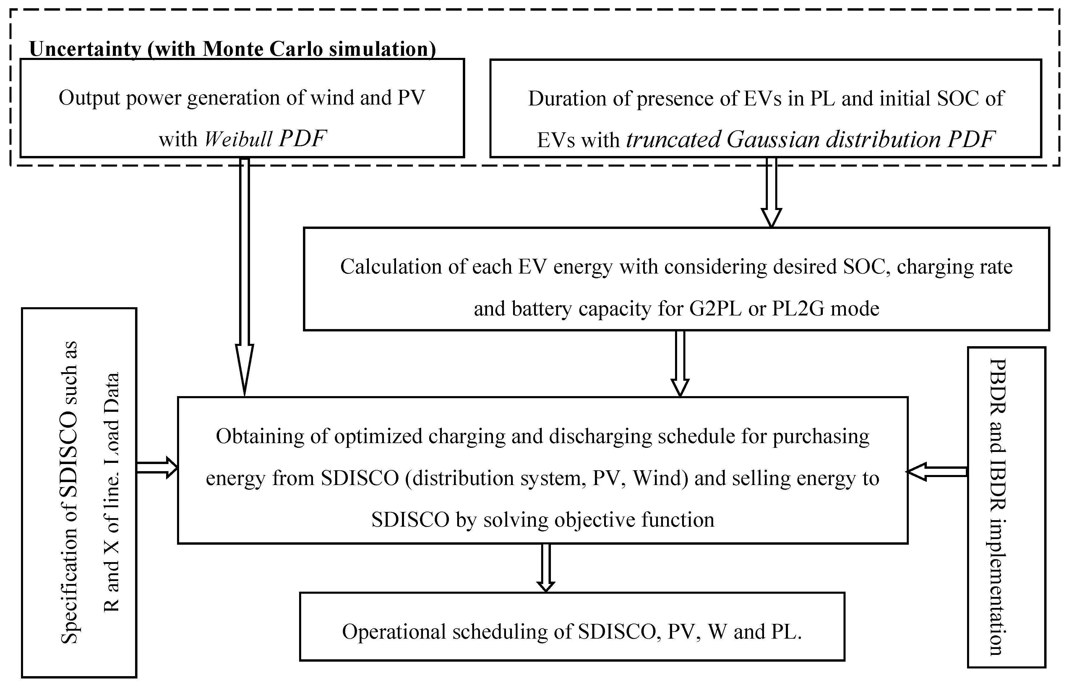
3.4. Problem Solving Process

Since this problem has different uncertainties, a stochastic programming is used to solve the objective function. The following five uncertainties are considered in this paper:

• Wind generating units’ uncertainty: Because wind speed is intermittent, many experiments prove that stochastic wind speed in many regions roughly pursues the Weibull PDF. The output of the wind unit can be obtained through the linear relationship between wind speed and wind turbine output [41].
• Solar generating sources uncertainty: Predominantly illumination intensity affects the output of PV. In [41], it is shown that the distribution of solar irradiance is characterized by using of Weibull PDF. The output of PV can be obtained through the linear relationship between irradiance and photovoltaic array output.
• Arrival time of EV to PL uncertainty
• Departure time of EV to PL uncertainty
• Initial SOC of EV uncertainty

Obtaining sufficient historical data for determining the exact PDF of the uncertainty in the estimation of initial SOC for the duration of the presence of EVs in PL is very difficult. However, most of the studies have reasonably suggested that a truncated Gaussian distribution PDF can be used [38].

Moreover, a scenario tree of all uncertainties is generated with the Monte Carlo method. Then, the scenarios are reduced with the concept of Kantorovich distance (K-distance). These are the binary and integer decision variables in the linear single-level model. Therefore, considering all the relations, the proposed model is the mixed-integer linear programming (MILP) problem. Therefore, in this paper, the simulation is carried out through the CPLEX solver of GAMS. The simulation has been implemented in a laptop with Core i7 up to 3.5 GHz CPU, 12 GB RAM (DDR4) and 4 MB cache. The flowchart of the stochastic programming-based operational scheduling of SDISCO is shown in Figure 2.

4. Numerical Results

For the case study, a standard IEEE 33-bus distribution system is considered over a 24-h period. The required data, such as modified load, resistance and reactance of lines and the maximum line current limit of this test system that is shown in Figure 3, are from [42].

The required specifications of the wind and PV unit are summarized in

Table 1. Considered data for the PV and wind unit.

Wind Unit
Size (kW)	bus	shape index	scale index	cut-in speed (m/s)	nominal speed (m/s)	cut-out speed (m/s)
500	16	2	6.5	4	14	25
PV Unit
Size (kW)	bus	shape index	scale index	rated illumination intensity (w.m2) 1000
500	14	1.8	5.5

[41]. Figure 4 shows the profiles of the PV and wind unit generation. The total generation of the PV and wind unit over a 24 h period is about 2.840 and 7.386 MWh, respectively.

The modified details of the EV’s probability distributions are expressed in

Table 2. Probability distribution of EVs.

	Mean	Standard Deviation	Min	Max
Initial SOC (%)	50	25	30	60
Arrival Time (h)	8	3	7	10
Departure Time (h)	20	3	18	24

. Furthermore, the PL is installed on Bus 11. It is amused that 500 EVs are parked in PL. The power factor of customer’s loads and wind and PV units is 0.95 lagging and one, respectively. The specification of EVs is explained in

Table 3. Required specifications of EVs.

charge efficiency	90%	battery capacity (kWh)	50	SOCmin (kWh)	7.5
discharge efficiency	95%	charging/discharging rate (kW-h)	10	SOCmax (kWh)	45
SOCdep (kWh)	45	Ccd ($/MWh)	30	PL bus	11

[38].

The price elasticity of the demand is considered, as listed in

Table 4. Self- and cross-elasticity.

	On-Peak	Mid-Peak	Off-Peak
On-peak (14–20)	−0.1	0.016	0.012
Mid-peak (8–13 and 21–22)	0.016	−0.1	0.01
Off-peak (1–7 and 23–24)	0.012	0.01	−0.1

[26]. In order to study the operational scheduling, TOU, CAP and combined TOU and CAP are considered, as respectively presented in

Table 5. The case considering PBDR and IBDR for operational scheduling of SDISCO. CAP, capacity market program.

Program	Electricity Price for Load, Charging/Discharging of EVs ($/MWh)	Incentive Value ($/MWh)	Penalty Value ($/MWh)
Base case	131.292 flat rate	0	0
TOU	65.646, 131.292, 262.584 at off-peak, mid-peak and on-peak respectively	0	0
CAP	131.292 flat rate	100	50
TOU + CAP	65.646, 131.292, 262.584 at off-peak, mid-peak and on-peak respectively	100	50

. The hourly prices of the energy market are extracted from [42]. Furthermore, suppose that 20% of customers participate in the DR programs, i.e., 20% of the total load.

At first, two extreme cases, i.e., risk-neutral (without taking into account risk, β = 0) and risk-averse (with fully taking into account risk, β = 1), are investigated from the SDISCO profit point of view. In

Table 6. The profit of different DR programs in β = 0, 1.

Program	Profit of SDISCO with β = 0	Profit of SDISCO with β = 1
Base case (flat)	1723.773	1628.860
TOU	2272.869	2152.032
CAP	1262.504	1142.833
TOU + CAP	1668.412	1501.835

are shown the results of the mentioned programs. Based on this table, TOU is the best program. Furthermore, with increasing β (taking into account risk), the amount of profit is reduced.

TOU is the best DR program, so in the following, by changing the β (zero and one), a more comprehensive review is carried out from the perspective of profit, customers’ load, power purchased from the wholesale market, power exchange between SDISCO and PL and losses.

Table 7. The amount of the revenue and cost in TOU programs (β = 0, 1).

β	0	1
Selling of energy to EV owners ($)	1821.981	1662.296
Selling of energy to load ($)	8500.808	8500.808
Providing power from wholesale market ($)	7285.033	7454.307
Energy purchased from EV owners for supplying load ($)	764.887	556.7639
Implementation of PBDR and IBDR programs ($)	0	0
Expected value (profit) ($)	2272.869	2152.032

indicates the costs and revenue in dollar terms, in the TOU program. Without the SDISCO taking into account the risk, i.e., β = 0, more power exchange with PL happens, which leads to buying less power from the wholesale market. In this situation, the profit of SDISCO is increased. Based on this table, by taking into account risk, total profit is reduced by about 5.28%. Furthermore, only the amount of selling of energy to the load is equal in the two cases, because the SDISCO must meet the customer’s demand. The customer’s load with/without the TOU program is shown in Figure 5. The reduction of demand is about 1.550 MWh by the implementation of this program.

The amount of power purchased from the wholesale market in the two cases is shown in Figure 6. Based on Figure 6, before the EVs’ arrival, some parts of the load are supplied by RERs generation. Furthermore, with the presence of EVs in PL at mid-peak and off-peak periods, charging of EVs occurs. In the on-peak period, i.e., 14–20, due to discharging of EVs for supplying customers’ load, the purchasing energy from the wholesale market is severely reduced. In addition to the SDISCO supplying load and charging of EVs in two cases, i.e., β = 0 and β = 1, about 63.278 and 63.323 MWh of energy is purchased from the wholesale market, respectively.

Smart charging/discharging scheduling of 500 EVs in PL in the two cases is shown in Figure 7. Based on Figure 7, the total amount of power for charging of EVs in β = 0 and β = 1 is 15.175 and 14.248 MWh, respectively. Furthermore, the amount of power that PL puts back into the grid (discharging power) in β = 0 and β = 1 is 2.912 and 2.120 MWh, respectively. The reason for the low amount of power discharging is that most of the EVs leave the PL from 20:00, and there is no time for recharging of EVs, so virtually, a large number of EVs does not participate in the discharging program. Moreover, at Hours 14, 15, 19 and 20, the price of wholesale market energy is lower than the price of discharging EVs’ energy. Therefore, the SDISCO prefers to purchase power from the wholesale market.

Table 8. The amount of the losses (kW).

Time	Losses		Time	Losses		Time	Losses		Time	Losses
	β = 0	β = 1		β = 0	β = 1		β = 0	β = 1		β = 0	β = 1
1	40.94	66.46	7	93.09	129.90	13	56.87	66.94	19	44.01	47.78
2	38.40	60.21	8	52.40	89.16	14	44.81	49.51	20	41.56	48.03
3	38.51	56.19	9	404.37	361.47	15	43.11	47.22	21	173.24	151.43
4	36.23	60.32	10	490.78	448.26	16	55.32	52.21	22	123.86	131.08
5	36.68	50.21	11	115.46	126.61	17	79.36	64.51	23	70.43	84.27
6	37.43	57.37	12	56.75	73.53	18	42.17	44.75	24	72.69	100.03

shows the amount of losses in these two cases. According to the table, charging/discharging of EVs increases/decreases the network losses. Furthermore, the total amount of losses in the β = 0 and β = 1 situations is 2.288 and 2.467 MW, respectively. Furthermore, since in the risk-averse mode, more power is purchased from the wholesale market, the network losses are increased.

Furthermore, the effect of the risk aversion parameter, i.e., β, on the optimal operational scheduling of SDISCO from the profit point of view is shown in

Table 9. Risk aversion parameter effect and solution time.

β	0	0.1	0.3	0.5	0.7	0.9	1
Expected value (Profit) ($)	2272.869	2260.782	2236.643	2189.526	2188.258	2163.444	2152.032
CVaR ($)	-	2147.061	2148.751	2130.190	2150.147	2151.239	2152.032
Solution time (s)	358.109	376.469	386.375	372.937	585.828	601.640	1670.344

. Based on this table, the reduction of profit and increase of CVaR are achieved by increasing β. Low/high levels of risk are associated with high/low expected profit. The solution time is also shown in this table. By β = 1, the problem is very complicated, and more time is needed for solving.

Finally, since there is volatility in the market price, the sensitivity analysis is carried out for investigating the effect of changing the electricity price on the SDISCO’s profit in β = 1. According to Figure 8, by increasing/decreasing the price of electricity, the profit of SDISCO decreases/increases. As a result, if the price of electricity is reduced 15%, the profit increases about 51%.

5. Conclusions

A new risk-based bi-level model for operational scheduling of SDISCO was presented in this paper to address the uncertainties with RERs and EVs. At each level, the aim was maximizing the profits. For solving the problem, KKT conditions and a method based on auxiliary binary variables and sufficiently large constants were used. Furthermore, TOU, CAP and combined TOU and CAP programs were considered. The results indicated that:

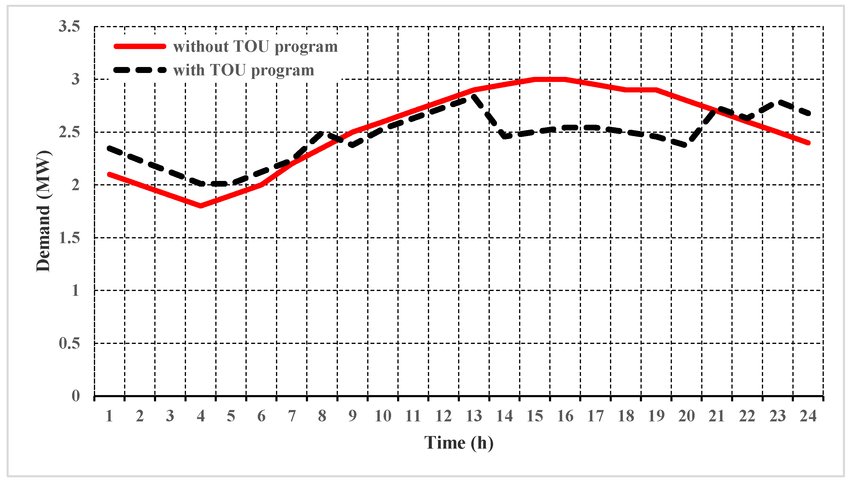
• In this model, in each case (with/without taking into account risk), by the implementation of the TOU program, the SDISCO achieved more profit due to selling more energy to the customers and PL.
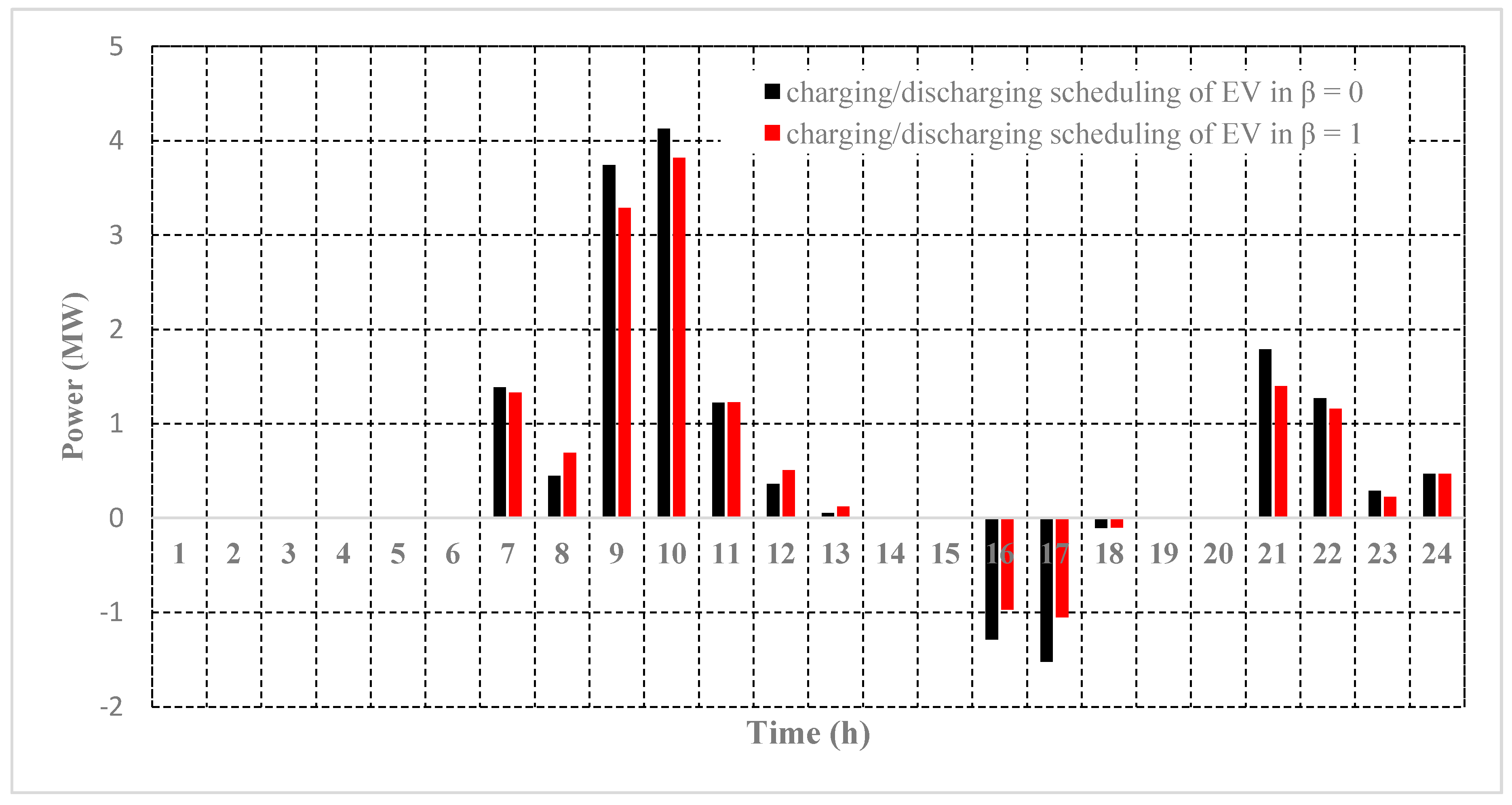
• By using proper charging/discharging scheduling of EVs, EVs’ charging was carried out at the off-peak or mid-peak periods. Moreover, EVs’ discharging occurred during the on-peak period. This discharging could not happen at 14:00, 15:00, 19:00 and 20:00, because in these time slots, the price of the EVs’ discharging power was higher than the one of the wholesale market, so the SDISCO preferred to provide energy from the wholesale market.
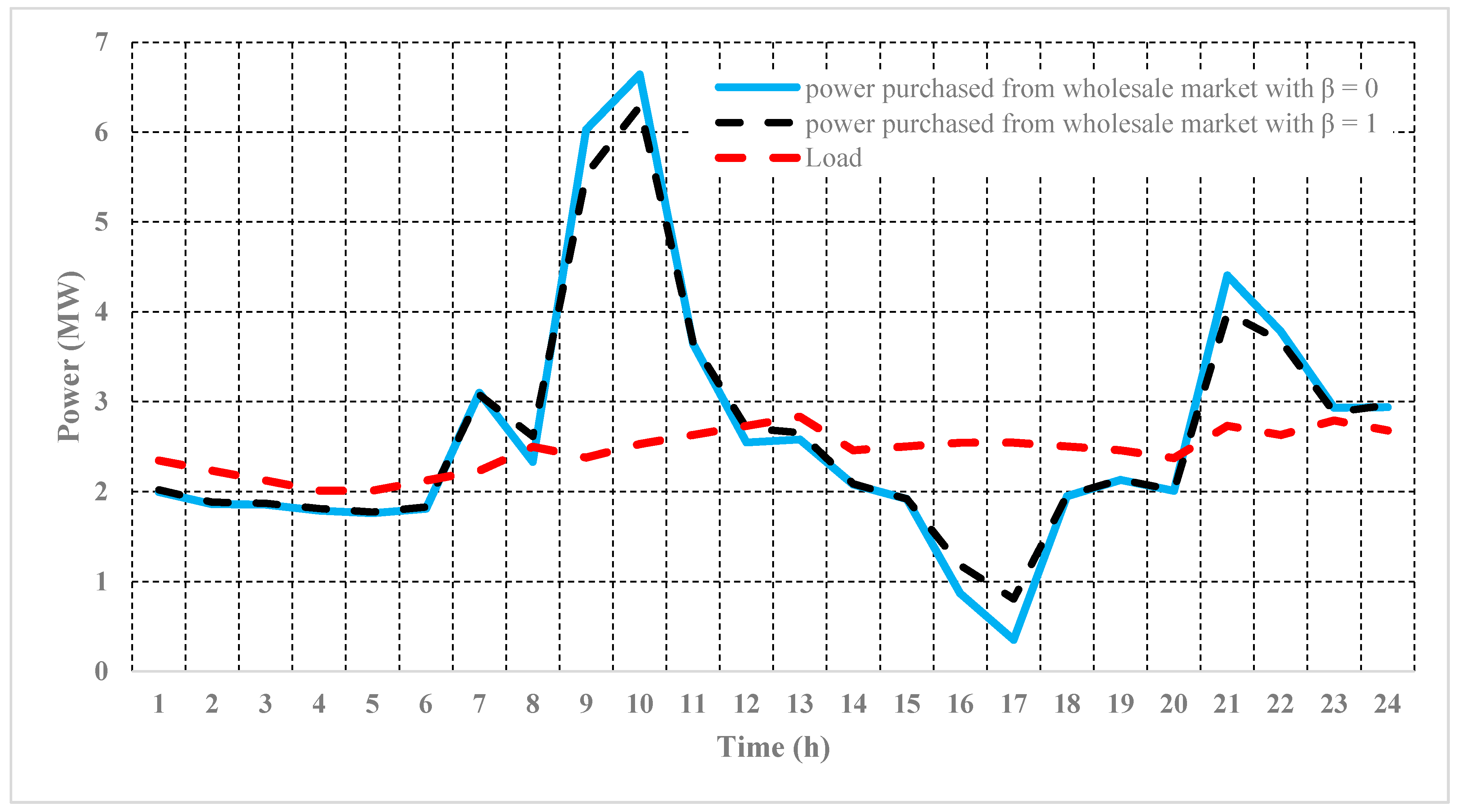
• By taking the risk into account, i.e., β = 1, SDISCO has obtained less profit, because of purchasing more energy from the wholesale market and also due to low charging/discharging of EVs.
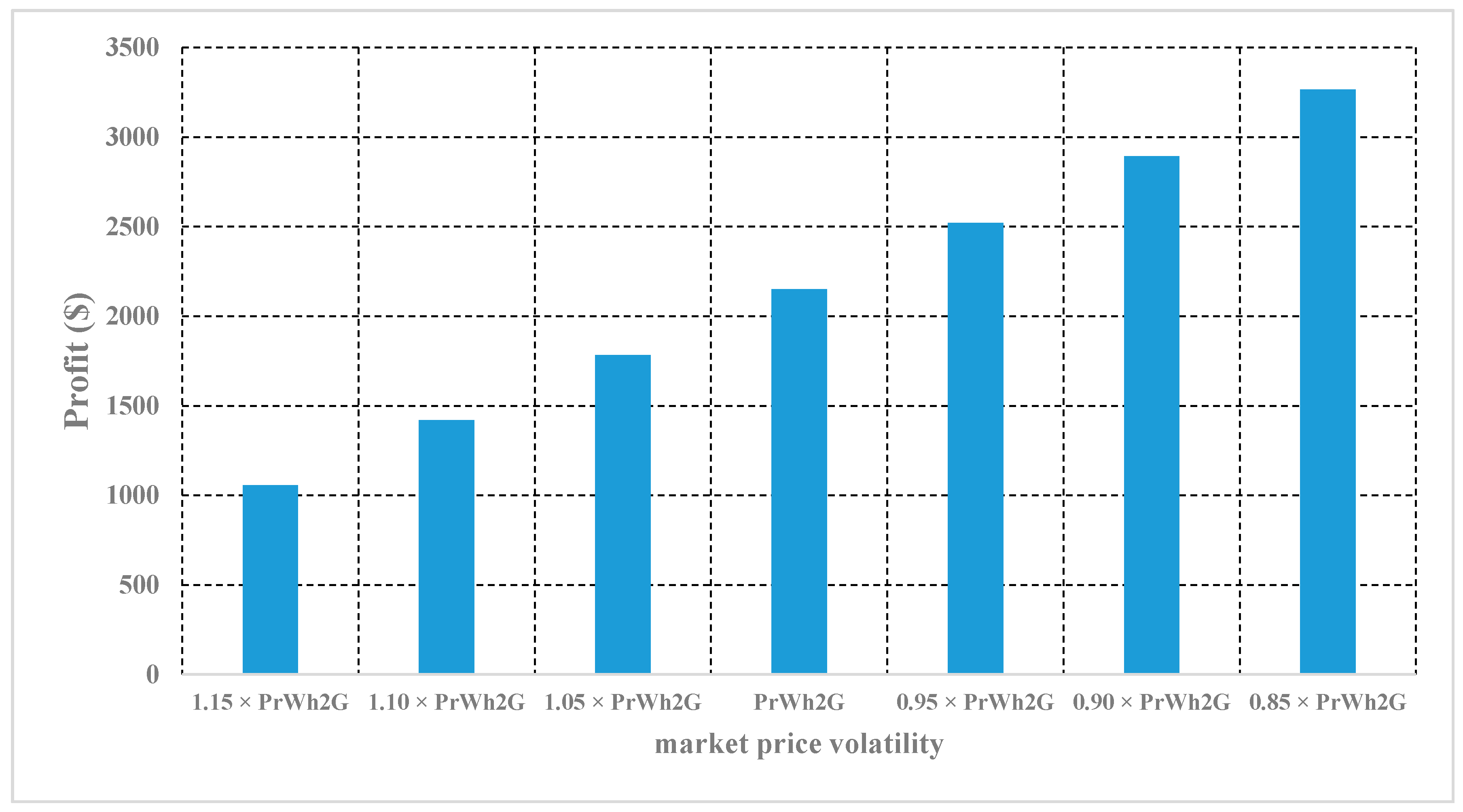
• By increasing/decreasing the price of electricity, the profit of SDISCO decreases/increases.

References

1. Fernandez, L.P.; San Román, T.G.; Cossent, R.; Domingo, C.M.; Frias, P. Assessment of the impact of plug-in electric vehicles on distribution networks. IEEE Trans. Power Syst. 2011, 26, 206–213. [Google Scholar] [CrossRef]
2. ElNozahy, M.S.; Salama, M.M.A. A comprehensive study of the impacts of PHEVs on residential distribution networks. IEEE Trans. Sustain. Energy 2014, 5, 332–342. [Google Scholar] [CrossRef]
3. Weiller, C. Plug-in hybrid electric vehicle impacts on hourly electricity demand in the United States. Energy Policy 2011, 39, 3766–3778. [Google Scholar] [CrossRef]
4. Mullan, J.; Harries, D.; Bräunl, T.; Whitely, S. Modelling the impacts of electric vehicle recharging on the Western Australian electricity supply system. Energy Policy 2011, 39, 4349–4359. [Google Scholar] [CrossRef]
5. Yong, J.Y.; Ramachandaramurthy, V.K.; Tan, K.M.; Mithulananthan, N. A review on the state-of-the-art technologies of electric vehicle, its impacts and prospects. Renew. Sustain. Energy Rev. 2015, 49, 365–385. [Google Scholar] [CrossRef]
6. Jiménez, A.; García, N. Voltage unbalance analysis of distribution systems using a three-phase power flow ans a Genetic Algorithm for PEV fleets scheduling. In Proceedings of the Power and Energy Society General Meeting, San Diego, CA, USA, 22–26 July 2012; pp. 1–8. [Google Scholar]
7. Shareef, H.; Islam, M.M.; Mohamed, A. A review of the stage-of-the-art charging technologies, placement methodologies, and impacts of electric vehicles. Renew. Sustain. Energy Rev. 2016, 64, 403–420. [Google Scholar] [CrossRef]
8. Salman, H.; Muhammad, K.; Umar, R. Impact analysis of vehicle-to-grid technology and charging strategies of electric vehicles on distribution networks—A review. J. Power Sources 2015, 277, 205–214. [Google Scholar]
9. Moses, P.S.; Deilami, S.; Masoum, A.S.; Masoum, M.A. Power quality of smart grids with plug-in electric vehicles considering battery charging profile. In Proceedings of the 2010 IEEE PES Innovative Smart Grid Technologies Conference Europe (ISGT Europe), Gothenburg, Sweden, 11–13 October 2010; pp. 1–7. [Google Scholar]
10. Razeghi, G.; Zhang, L.; Brown, T.; Samuelsen, S. Impacts of plug-in hybrid electric vehicles on a residential transformer using stochastic and empirical analysis. J. Power Sources 2014, 252, 277–285. [Google Scholar] [CrossRef]
11. Akhavan-Rezai, E.; Shaaban, M.F.; El-Saadany, E.F.; Zidan, A. Uncoordinated charging impacts of electric vehicles on electric distribution grids: Normal and fast charging comparison. In Proceedings of the Power and Energy Society General Meeting, San Diego, CA, USA, 22–26 July 2012; pp. 1–7. [Google Scholar]
12. Aziz, M.; Oda, T.; Mitani, T.; Watanabe, Y.; Kashiwagi, T. Utilization of Electric Vehicles and Their Used Batteries for Peak-Load Shifting. Energies 2015, 8, 3720–3738. [Google Scholar] [CrossRef]
13. Lotfy, M.E.; Senjyu, T.; Farahat, M.A.-F.; Abdel-Gawad, A.F.; Matayoshi, H. A Polar Fuzzy Control Scheme for Hybrid Power System Using Vehicle-To-Grid Technique. Energies 2017, 10, 1083. [Google Scholar] [CrossRef]
14. Bhattarai, B.P.; Myers, K.S.; Bak-Jensen, B.; Paudyal, S. Multi-Time Scale Control of Demand Flexibility in Smart Distribution Networks. Energies 2017, 10, 37. [Google Scholar] [CrossRef]
15. Zakariazadeh, A.; Shahram, J.; Pierluigi, S. Multi-objective scheduling of electric vehicles in smart distribution system. Energy Convers. Manag. 2014, 79, 43–53. [Google Scholar] [CrossRef]
16. Lorf, C.; Martínez-Botas, R.F.; Howey, D.A.; Lytton, L.; Cussons, B. Comparative analysis of the energy consumption and CO2 emissions of 40 electrics, plug-in hybrid electric, hybrid electric and internal combustion engine vehicles. Transp. Res. Part D Transp. Environ. 2013, 23, 12–19. [Google Scholar] [CrossRef]
17. Sioshansi, R.; Miller, J. Plug-in hybrid electric vehicles can be clean and economical in dirty power systems. Energy Policy 2011, 39, 6151–6161. [Google Scholar] [CrossRef]
18. Tulpule, P.J.; Marano, V.; Yurkovich, S.; Rizzoni, G. Economic and environmental impacts of a PV powered workplace parking garage charging station. Appl. Energy 2013, 108, 323–332. [Google Scholar] [CrossRef]
19. Marra, F.; Yang, G.Y.; Træholt, C.; Larsen, E.; Østergaard, J.; Blažič, B.; Deprez, W. EV charging facilities and their application in LV feeders with photovoltaics. IEEE Trans. Smart Grid 2013, 4, 1533–1540. [Google Scholar] [CrossRef]
20. Luo, X.; Xia, S.; Chan, K.W. A decentralized charging control strategy for plug-in electric vehicles to mitigate wind farm intermittency and enhance frequency regulation. J. Power Sources. 2014, 248, 604–614. [Google Scholar] [CrossRef]
21. Wu, T.; Yang, Q.; Bao, Z.; Yan, W. Coordinated energy dispatching in microgrid with wind power generation and plug-in electric vehicles. IEEE Trans. Smart Grid 2013, 4, 1453–1463. [Google Scholar] [CrossRef]
22. Su, W.; Wang, J.; Roh, J. Stochastic energy scheduling in microgrids with intermittent renewable energy resources. IEEE Trans. Smart Grid 2014, 5, 1876–1883. [Google Scholar] [CrossRef]
23. Jin, C.; Sheng, X.; Ghosh, P. Optimized electric vehicle charging with intermittent renewable energy sources. IEEE J. Sel. Top. Signal Process. 2014, 8, 1063–1072. [Google Scholar] [CrossRef]
24. Aalami, H.; Yousefi, G.R.; Moghadam, M.P. Demand response model considering EDRP and TOU programs. In Proceedings of the Transmission and Distribution Conference and Exposition, T&D. IEEE/PES, Chicago, IL, USA, 21–24 April 2008; pp. 1–6. [Google Scholar]
25. Aalami, H.A.; Moghaddam, M.P.; Yousefi, G.R. Demand response modeling considering interruptible/curtailable loads and capacity market programs. Appl. Energy 2010, 87, 243–250. [Google Scholar] [CrossRef]
26. Aalami, H.A.; Moghaddam, M.P.; Yousefi, G.R. Modeling and prioritizing demand response programs in power markets. Electr. Power Syst. Res. 2010, 80, 426–435. [Google Scholar] [CrossRef]
27. Conejo, A.J.; Carrión, M.; Morales, J.M. Decision Making Under Uncertainty in Electricity Markets; Springer: New York, NY, USA, 2010; Volume 1, Available online: http://www.springer.com/gp/book/9781441974204 (accessd on 23 September 2017).
28. Alipour 2010, M.; Mohammadi-Ivatloo, B.; Zare, K. Stochastic risk-constrained short-term scheduling of industrial cogeneration systems in the presence of demand response programs. Appl. Energy 2014, 136, 393–404. [Google Scholar] [CrossRef]
29. Tan, Z.; Wang, G.; Ju, L.; Tan, Q.; Yang, W. Application of CVaR risk aversion approach in the dynamical scheduling optimization model for virtual power plant connected with wind-photovoltaic-energy storage system with uncertainties and demand response. Energy 2017, 124, 198–213. [Google Scholar] [CrossRef]
30. Dolatabadi, A.; Mohammadi-Ivatloo, B. Stochastic risk-constrained scheduling of smart energy hub in the presence of wind power and demand response. Appl. Therm. Eng. 2017, 123, 40–49. [Google Scholar] [CrossRef]
31. Esmaeeli, M.; Kazemi, A.; Shayanfar, H.; Chicco, G.; Siano, P. Risk-based planning of the distribution network structure considering uncertainties in demand and cost of energy. Energy 2017, 119, 578–587. [Google Scholar] [CrossRef]
32. Esmaeeli, M.; Kazemi, A.; Shayanfar, H.; Haghifam, M.R.; Siano, P. Risk-based planning of distribution substation considering technical and economic uncertainties. Electr. Power Syst. Res. 2016, 135, 18–26. [Google Scholar] [CrossRef]
33. Larimi, S.M.M.; Haghifam, M.R.; Moradkhani, A. Risk-based reconfiguration of active electric distribution networks. IET Gener. Transm. Distrib. 2016, 10, 1006–1015. [Google Scholar] [CrossRef]
34. Bahramara, S.; Moghaddam, M.P.; Haghifam, M.R. Modelling hierarchical decision making framework for operation of active distribution grids. IET Gener. Transm. Distrib. 2015, 9, 2555–2564. [Google Scholar] [CrossRef]
35. Bahramara, S.; Moghaddam, M.P.; Haghifam, M.R. A bi-level optimization model for operation of distribution networks with micro-grids. Int. J. Electr. Power Energy Syst. 2016, 82, 169–178. [Google Scholar] [CrossRef]
36. Cai, Y.; Lin, J.; Wan, C.; Song, Y. Stochastic Bi-level Trading Model for an Active Distribution Company with DGs and Interruptible Loads. IET Renew. Power Gener. 2016, 11, 278–288. [Google Scholar] [CrossRef]
37. Kardakos, E.G.; Simoglou, C.K.; Bakirtzis, A.G. Optimal offering strategy of a virtual power plant: A stochastic bi-level approach. IEEE Trans. Smart Grid 2016, 7, 794–806. [Google Scholar] [CrossRef]
38. Shafie-khah, M.; Siano, P.; Fitiwi, D.Z.; Mahmoudi, N.; Catalão, J.P. An Innovative Two-Level Model for Electric Vehicle Parking Lots in Distribution Systems with Renewable Energy. IEEE Trans. Smart Grid 2017, PP, 1. [Google Scholar] [CrossRef]
39. Carrion, M.; Arroyo, J.M.; Conejo, A.J. A bilevel stochastic programming approach for retailer futures market trading. IEEE Trans. Power Syst. 2009, 24, 1446–1456. [Google Scholar] [CrossRef]
40. Dempe, S.; Kalashnikov, V.; Pérez-Valdés, G.A.; Kalashnykova, N. Bilevel Programming Problems: Theory, Algorithms and Applications to Energy Networks; Springer: Berlin/Heidelberg, Germany, 2015. [Google Scholar]
41. Liu, Z.; Wen, F.; Ledwich, G. Optimal siting and sizing of distributed generators in distribution systems considering uncertainties. IEEE Trans. Power Deliv. 2011, 26, 2541–2551. [Google Scholar] [CrossRef]
42. Mazidi, M.; Monsef, H.; Siano, P. Robust day-ahead scheduling of smart distribution networks considering demand response programs. Appl. Energy 2016, 178, 929–942. [Google Scholar] [CrossRef]
Figure 1. Demand response (DR) programs.
Energies 10 01714 g001
Figure 2. Process solving of operational scheduling of smart distribution company (SDISCO). PBDR, price-based demand response; IBDR, incentive-based DR.
Energies 10 01714 g002
Figure 3. The 33-bus distribution system.
Energies 10 01714 g003
Figure 4. PV and wind power generation.
Energies 10 01714 g004
Figure 5. Demand of the customer with/without the TOU program.
Energies 10 01714 g005
Figure 6. Power purchased from the wholesale market in the two cases.
Energies 10 01714 g006
Figure 7. Charging/discharging scheduling of 500 EVs.
Energies 10 01714 g007
Figure 8. SDISCO’s profit in β = 1 by changing of PrWh2G.
Energies 10 01714 g008