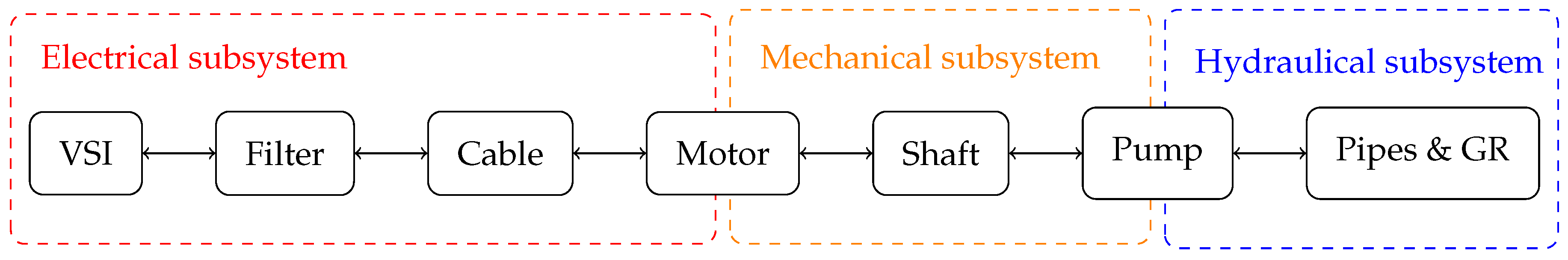
The electrical subsystem covers the inverter, sine filter, cable and motor. Based on three-phase equivalent circuits, a two-phase description is derived for each component, yielding expressions for the inputs and output currents and (phase) voltages, respectively. The phase voltages are stated with respect to the reference potential measured at the motor star point , which is further specified in the motor section.
2.1.1. Inverter
The power converter links the grid with the electrical drive system and is typically given in back-to-back configuration, with a grid-side voltage source inverter (VSI), a common DC-link and a motor-side VSI. Instead of the grid-side VSI (active front end), which allows bidirectional power flow, a diode bridge may alternatively be used as a rectifier, if the electric power is supposed to flow from the grid to the machine only. The model derived in this paper assumes a constantly charged DC-link capacitance (see Assumption 2) and hence restrains to the motor side. The motor-side VSI serves as a voltage and power source for the electrical machine of the pump, generating sinusoidal voltages of variable frequency and amplitude according to a specified reference voltage. In this paper a 5-level active neutral point clamped (ANPC-5L) inverter as described in [
19] is employed, which is well-suited for medium voltage drive applications.
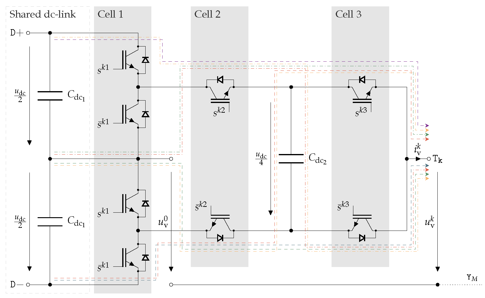
The schematic of a single phase
of the inverter is depicted in
Figure 2. Each phase
a,
b or
c of the inverter consists of three cascaded cells with a total of eight power switches per phase. The input is accessed via the terminals
and
while the output voltages are taken from the terminals
, respectively. Moreover, the phase current
flows out of the inverter. The power switches of phase
k—typically given as insulated-gate bipolar transistors (IGBT)—are controlled by the three switching signals
(the respective inverse signals are denoted by
,
and
). Cell 1 is controlled by switching signal
, with switches 1 and 3 (counted from top to bottom) and switches 2 and 4 controlled in pairs. Cell 2 consists of two complementary switches controlled by
, as does cell 3 which in turn is controlled by
.
Assumption 1 (Ideal switches).
The inverter IGBTs are assumed ideal switches with switching levels ’1’ (closed) and ’0’ (open), i.e.,
no current may flow if the switch is open,
bidirectional current may flow without voltage drop, if the switch is closed and
the switching takes place instantaneously (no switching delay).
The input DC-link capacitances
are shared between the three phases, whereas the capacitance
is assigned to each phase individually [
19]. While
is charged by the grid-side rectifier or VSI,
is charged by exploiting redundant switching-states and thus controlling the current flowing into or out of the capacitance (i.e., “voltage balancing”). As sophisticated inverter control algorithms are beyond the scope of this paper, the following assumption is made.
Assumption 2 (VSI capacitance).
The inverter capacitances and are charged to defined voltage levels and and are assumed constant for all times.
The switching combinations and resulting output voltages of phase
k are listed in
Table 1. The corresponding current paths are indicated in
Figure 2 by the colored lines, which comply with the background colors of the table rows. Although three switches allow for eight different switching combinations, the line-to-neutral voltage
(in
) measured between the output terminal
and the neutral point
can attain five distinct voltage levels, i.e.,
. This aforementioned redundancy can be used to charge the phase capacitance
. However, the exact switching combinations leading to the different voltage levels are irrelevant for the model presented in this paper and therefore the overall switching signal
is used to summarize and describe the overall switching-state and its respective output voltage level for phase
k.
Hence, the overall three-phase switching-state vector
can be introduced such that the line-to-neutral voltages
may be written as:
The line-to-line voltages
measured between the inverter outputs
,
and
(see
Figure 2) can in turn be expressed in terms of the line-to-neutral voltages as:
yielding nine different output voltage levels, i.e.,
. Moreover, the line-to-line voltages may be expressed as
, where
are the phase voltages measured between the output terminals of the inverter and the motor star point
. Since the matrix
is not invertible, the equation cannot be solved for
[
20], Chapter 14. However, making use of the general voltage constraint
(with possibly non-zero offset voltage
, if the phase voltages are not balanced), the phase voltages can be stated as:
As a two-phase representation is preferred here, the reduced amplitude-correct Clarke transformation and its (pseudo) inverse are introduced as (see e.g., [
20], Chapter 14)
Employing the transformation matrices defined in (
4), vectors may be transformed by
and matrices by
, respectively. Finally, the phase voltages and currents at the inverter output can be expressed in
-coordinates as
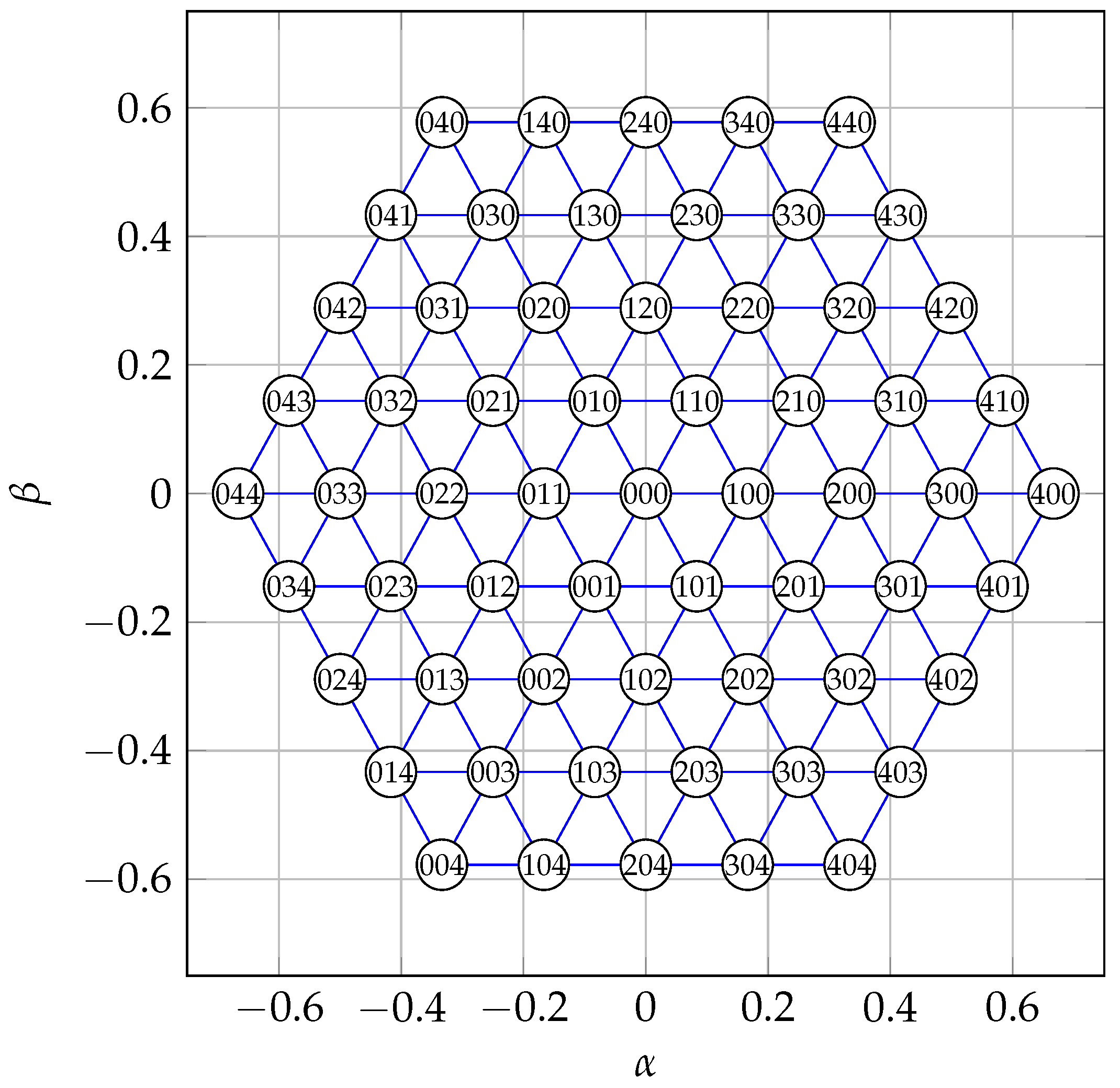
In the
-reference frame, the feasible phase voltages can be visualized by the voltage hexagon as shown in
Figure 3. The respective switching combinations
leading to each node are given in the circles attached to them (e.g.,
).
In general, the objective of the VSI is to reproduce a given voltage reference vector
at its output terminals. In order to achieve this goal, the desired voltage is sampled with switching frequency
(in
) and translated into the time domain by modulation of the switching signal, using e.g., sinusoidal pulse width modulation (SPWM) or space vector modulation (SVM). As a result, the sliding time integral (moving average) of the output voltages over a defined sampling period
(in
) matches the reference voltage sample, i.e.,:
A space vector modulation algorithm for 5-level inverters has been implemented based on [
21].
2.1.2. Filter
The VSI generates voltage pulses with steep slopes (high
) which (i) increase harmonic losses and (ii) put high stress on the insulation due to parasitic cable and motor capacitances [
22]. Moreover, the high inductance of the motor windings causes (iii) wave reflection at the machine terminals with a reflection factor of almost one [
23], requiring a voltage derating since the reflected voltage may reach twice the original amplitude [
23]. An effective way of avoiding the mentioned effects is to employ an LC ouput filter (lowpass filter) that smoothes the output voltages and thus reduces steep voltage slopes. The output filter is located between the VSI output and the downhole cable (see
Figure 1).
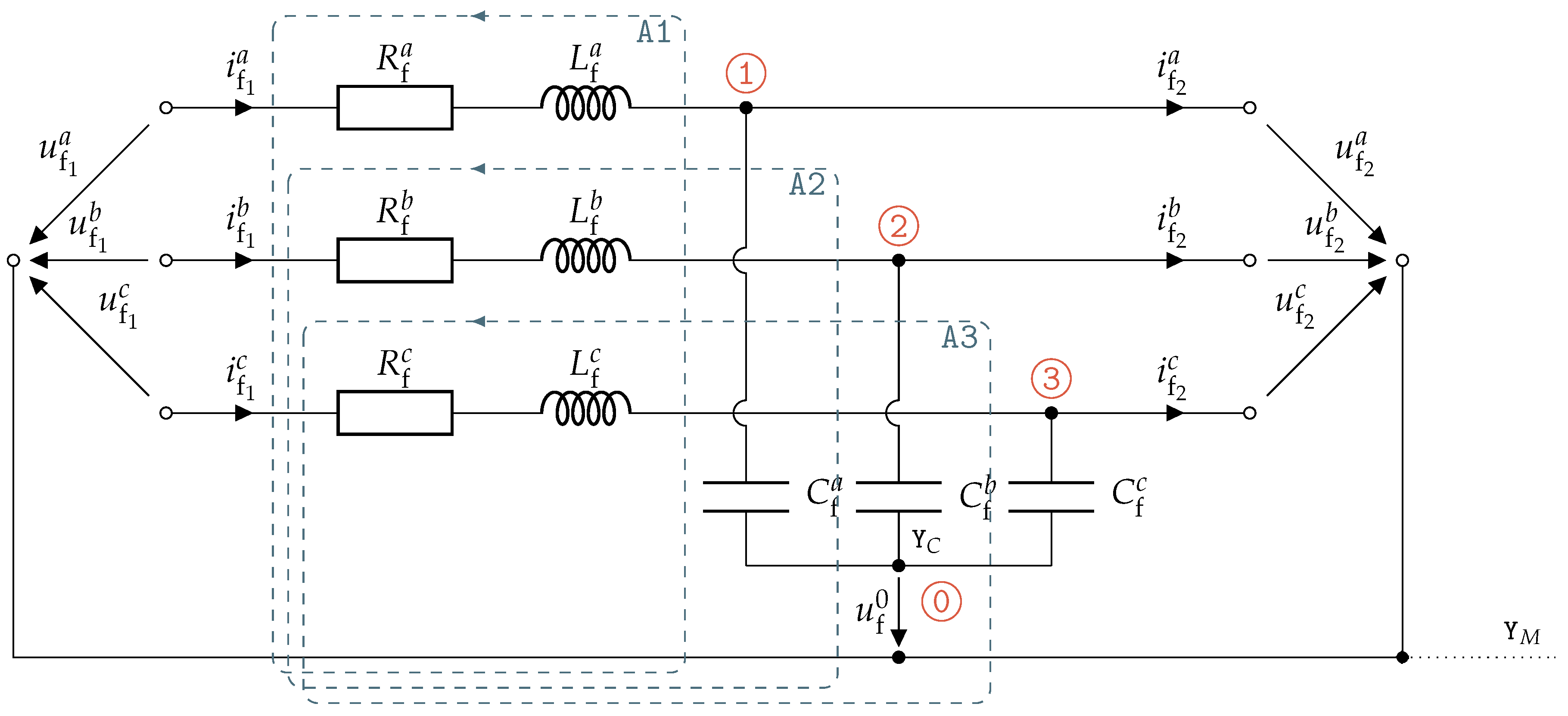
The equivalent circuit of a non-ideal LC-filter is shown in
Figure 4. The filter resistance matrix is given by
(in
), the filter inductance matrix by
(in
) and the filter capacitance matrix by
(in
).
The star point of the wye-connected capacitances is not grounded and hence at floating potential, i.e., at voltage with respect to the motor star point. Moreover, the input voltages are denoted by (in ), the input currents by (in ), the output voltages by (in ) and the output currents by (in ).
Using Kirchhoff’s current and voltage laws on nodes
⓪ to
③ and meshes
![Energies 10 01659 i001]()
to
![Energies 10 01659 i002]()
, respectively, yields
where
is the voltage between star point
of the capacitor bank and the star point
of the motor. Since
, the term ⊛ in (
8) vanishes if the reduced Clarke transformation is applied, thus yielding the reduced state-space representation in the
-reference:
with state vector
, input vector
, system matrix
and input matrix
. Note, that the input voltage vector
is equal to the VSI output vector
and the output current vector
depends on the load connected to the filter output.
2.1.3. Cable
The power cable connects the filter output with the electrical machine and runs through the space between wellbore and production tubing. As it extends over the whole distance, from the filter output to the motor, the cable length (in ) becomes a crucial parameter regarding the electrical properties of the cable such as resistance, inductance and capacitance, also known as line parameters and typically stated per-unit-length (p.u.l.).
The standard models for power transmission lines are derived by invoking a distributed parameters approach, which allows the modelling of an infinitesimally short fraction of the cable as a combination of p.u.l. series impedance and shunt admittance. This approach leads to a set of partial differential equations, called
Telegrapher’s equations (see e.g., [
24]), whose steady-state solution are time and space dependent wave functions for voltages and currents, respectively. As the distributed parameters approach leads to an infinitely large number of states, a discretization of the model using lumped parameters and a finite set of cable segments is performed. For sufficiently short segments the space dependency can be neglected and the segments can be approximated by equivalent
- or
-circuits. A segment is classified short if the wavelength
(in
) of the voltage and current waveforms is at least 60 times larger than the segment length, i.e.,
holds [
25], p. 426. Given the vacuum speed of light
(in
), the relative permeability of the cable insulation
and the frequency of the driving signals
f, the condition can be refined to (see [
25], p. 410):
It can be concluded from (
10) that, even without a sine filter and switching harmonics of up to 2
, the maximum cable length of
covers most geothermal power applications and hence a single sequence of
- and
-segments is sufficient for modeling the cable.
Nevertheless, in the presented model two segments are used: A -segment of length is used on the filter side, as the input voltage is a state variable due to the output capacitance of the filter, and a -segment of length is used on the load side of the cable, due to the input inductance of the electric machine. Considering the electric and magnetic coupling between the conductors, the circuit elements are derived from the p.u.l. line parameters.
Assumption 3 (Cable shunt conductance).
It is assumed that the shunt conductance of the power cable is negligible [25], p. 430. The remaining line parameters are given by (in ), (in ) and (in ), denoting the p.u.l. cable resistance, inductance and capacitance matrices.
Magnetic coupling is described by the p.u.l. inductance matrix which is defined as the constant ratio of conductor flux linkages and currents (if magnetic saturation is neglected), divided by the segment length
, i.e.,:
Moreover, electric coupling is represented by capacitances between the lines and ground, respectively. It can be shown (see
Appendix B and [
26]) that the capacitances used in the equivalent circuits, i.e., the line-to-ground capacitances
and line-to-line capacitances
(in
) for
, are related to the line capacitances used in the phase description by:
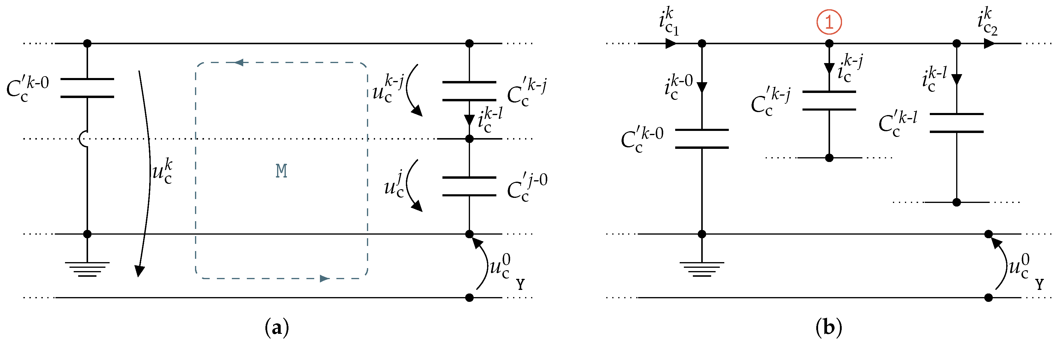
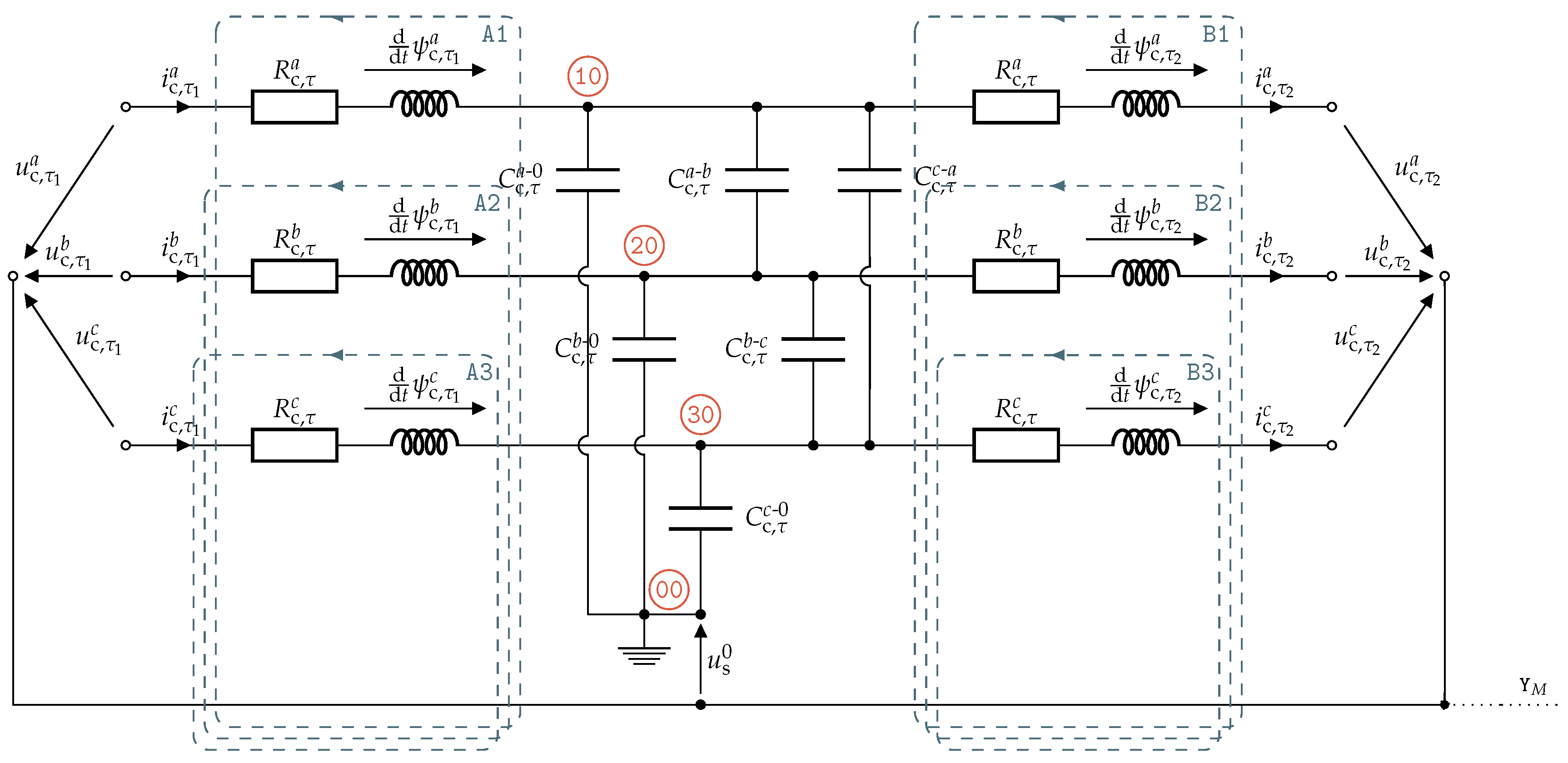
The equivalent circuit of the
-segment is shown in
Figure 5, with input voltages
(in
), input currents
(in
), output voltages
(in
), output currents
(in
) and voltages across the capacitances
(in
). Moreover, the
-model parameters are given by
(in
),
(in
) and
(in
). Note that, for inductances and resistances, half of the respective values were considered on the input and the other half on the output of the
-segment (that is why
appears in the expressions above).
As in the previous section, the state-space description can be derived using circuit analysis. For the
-model, evaluating meshes
![Energies 10 01659 i001]()
to
![Energies 10 01659 i002]()
, meshes
![Energies 10 01659 i003]()
to
![Energies 10 01659 i004]()
and nodes
![Energies 10 01659 i005]()
to
![Energies 10 01659 i006]()
yields
where
denotes the voltage between motor star point
and ground. Applying the reduced Clarke transformation as in (
4) eliminates the term ⊛, i.e.,
, such that the state-space description of the
-segment in the
-reference frame can be stated as
with state vector
, input vector
, system matrix
and input matrix
. For the
-segment, the input voltage
is equal to the filter output
and the output voltage
is determined by the input voltage of the
-segment.
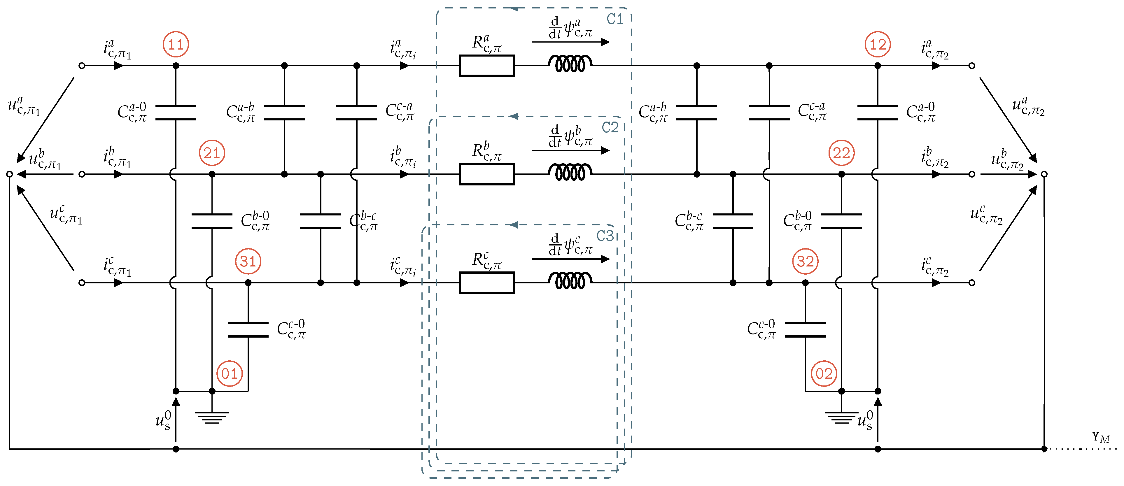
Likewise, the
-model state-space form can be derived. The equivalent circuit of the
-segment is shown in
Figure 6, with input voltages
(in
), input currents
(in
), output voltages
(in
), output currents
(in
) and currents through the inductances
(in
). The
-model parameters are given by
(in
), and
(in
) and
(in
).
The system description is obtained by evaluating meshes
![Energies 10 01659 i007]()
to
![Energies 10 01659 i008]()
, nodes
![Energies 10 01659 i009]()
to
![Energies 10 01659 i010]()
and
![Energies 10 01659 i011]()
to
![Energies 10 01659 i012]()
, i.e.,
Applying the reduced Clarke transformation, the disturbance ⊛ is eliminated, i.e.,
, and the state-space description for the
-segment is given by
with state vector
, input vector
, system matrix
and input matrix
. For the
-segment the input currents
are determined by the output currents of the
-segment, whereas the output currents
depend on the load connected at the cable end.
2.1.4. Electrical Machine
The electrical machine drives the pump. Both are mechanically linked via a shaft. In order to achieve higher power output, two separate motors may be connected in series, which is known as
tandem configuration [
27]. Typically, squirrel-cage induction motors are used, since they are well-known, cheap and robust. However, as high currents are flowing through the rotor bars and resistive losses (heat) are proportional to the current squared, induction machines tend to heat up quickly. Moreover, the only feasible way to cool the machine is the use of
hot geothermal fluid to conduct away the heat. Therefore, the ampere rating has to be kept at a minimum level, which requires a higher voltage rating of the machine in order to guarantee the desired mechanical output power.
Due to space limitations inside the borehole, the motor dimensions have to be adapted, resulting in a long axial expansion and a small diameter. While the stator windings typically expand over the whole length of the motor, the rotor on the other hand is segmented, with each segment isolated from each other and equipped with its own bearings [
28]. Moreover, the space between rotor and stator is filled with oil as to (i) prevent water from entering the machine, to (ii) accommodate the high ambient pressure and to (iii) improve heat transfer from the rotor to the motor surface in radial direction [
28].
Assumption 4 (Motor modeling).
It is assumed that
the motor is star-connected, i.e. the secondary ends of the phase windings are interconnected at the motor star point ,
the multi-rotor configuration can be considered a single rotor with combined electromagnetic properties, i.e., no torsional effects among individual rotors are considered, and
iron losses can be neglected.
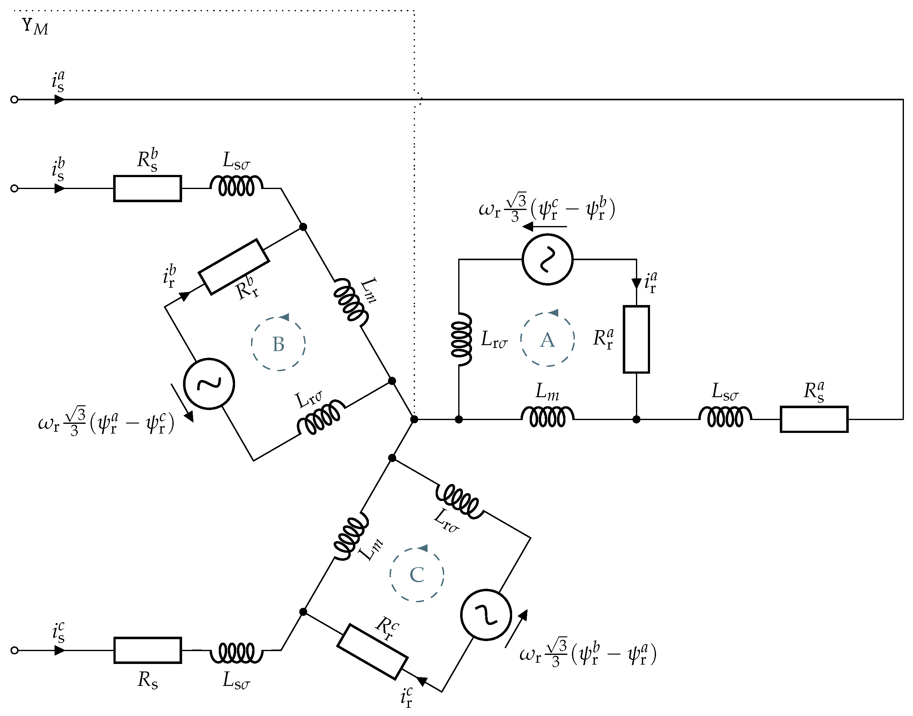
The resulting three-phase equivalent circuit is shown in
Figure 7, with stator voltages
(in
), stator currents
(in
) and stator flux linkages
(in
), rotor currents
(in
), rotor flux linkages
(in
) and rotor angular velocity
(in
), respectively. The rotor variables are related to the stator [
29] and expressed in stator fixed
-coordinates.
The stator windings (phases) are modeled by the stator resistances
(in
) and the stator inductance
(in
), where
can be separated into the stator stray inductance
(in
) and the main inductance
(in
), i.e.,
[
29]. The main inductance causes magnetic coupling between the rotor and stator phases which can be expressed in terms of the stator and rotor flux linkages.
Assumption 5 (Magnetic linearity).
It is assumed that the effect of magnetic saturation can be neglected and hence the stator and rotor flux linkages are affine functions of the stator and rotor currents, respectively, i.e., In the fault-free case, the phase resistances are typically identical, i.e., holds. However, in case of windage faults this assumption may not hold true anymore and therefore the general description is used in the presented model. For the sake of consistency, the same applies for the rotor resistances.
The stator voltages, measured between the input terminals and the motor star point
, are given by:
Applying the Clarke transformation (
4) yields the corresponding representation in the
-reference frame:
On the rotor side, the conducting bars of the rotor cage are likewise modeled as a three-phase system, with rotor resistance
(in
) and rotor inductance
, composed of the rotor stray inductance
(in
) and the main inductance
, i.e.,
[
29]. Moreover, the rotor magnetic field induces a voltage in the rotor cage depending on the flux linkage
and the electrical (synchronous) speed
, where
(in
) is the mechanical speed and
is the number of pole pairs. Evaluating meshes
![Energies 10 01659 i016]()
,
![Energies 10 01659 i017]()
and
![Energies 10 01659 i018]()
yields the following dependency:
which, transformed to
-coordinates, becomes:
where
and:
Solving (
22) for
allows to eliminate the rotor currents from (
19) and (
21) and, hence, the overall nonlinear state-space electrical system can be derived as follows:
where
denotes the inductive leakage factor,
is the state vector,
is the input vector,
is the non-linear system function and
is the input function. Note that the rotational speed
describes an additional system state which results from the torque balance on the machine shaft, i.e.,:
where
(in
) is the overall moment of inertia,
(in
) is the motor torque and
(in
) is the sum of load torques acting against the motor torque. In anticipation of the mechanical subsystem, the electro-magnetic torque
(in
) produced by the motor can be described in terms of electrical system states, i.e., (see e.g., [
20], Chapter 14):
The load torque and inertia, however, are determined by the hydraulic and mechanical subsystems derived in
Section 2.2 and
Section 2.3. Therefore, the rotational speed dynamics will be further elucidated in the following sections.


 to
to  , respectively, yields
 to
to  and nodes
  to
to  yields
 to
to  , nodes
  to
to  and
and  to
to  , i.e.,
 ,
,  and
and  yields the following dependency:
 is drawn, comprising the capacitances between phase a and ground, between phase b and ground and between phase a and b, respectively. Applying Kirchhoff’s voltage law yields:


 ] and [
  ]; (b) cable transfer function [
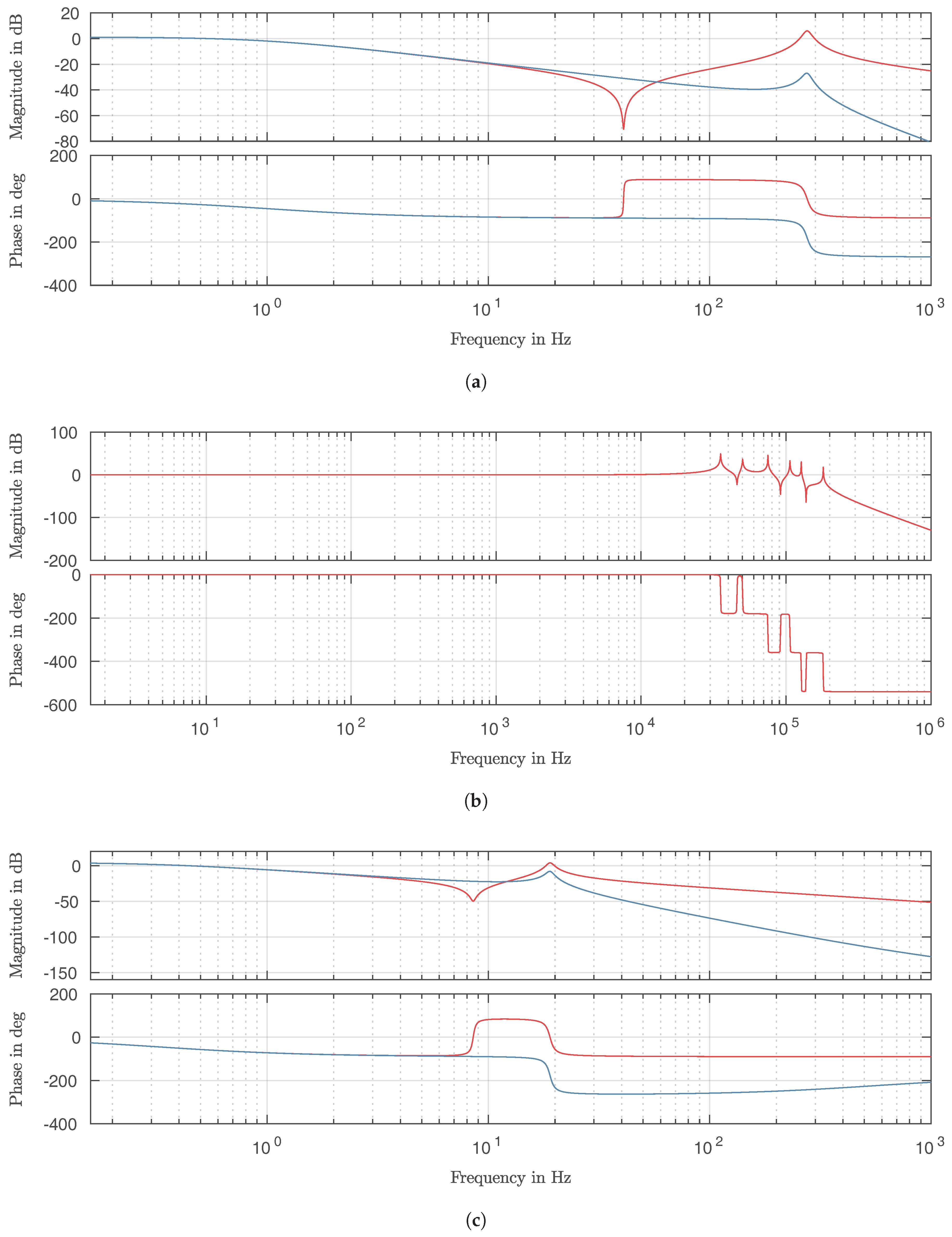
