Effect of Injection Site on Fault Activation and Seismicity during Hydraulic Fracturing

1
Key Laboratory of Deep Coal Resource, Ministry of Education of China, School of Mines, China University of Mining and Technology, Xuzhou 221116, China
2
Faculty of Engineering and Information Sciences, University of Wollongong, Wollongong 2522, Australia
*
Author to whom correspondence should be addressed.
Energies 2017, 10(10), 1619; https://doi.org/10.3390/en10101619
Submission received: 8 August 2017
/
Revised: 12 October 2017
/
Accepted: 12 October 2017
/
Published: 16 October 2017
Abstract
:Hydraulic fracturing is a key technology to stimulate oil and gas wells to increase production in shale reservoirs with low permeability. Generally, the stimulated reservoir volume is performed based on pre-existing natural fractures (NF). Hydraulic fracturing in shale reservoirs with large natural fractures (i.e., faults) often results in fault activation and seismicity. In this paper, a coupled hydro-mechanical model was employed to investigate the effects of injection site on fault activation and seismicity. A moment tensor method was used to evaluate the magnitude and affected areas of seismic events. The micro-parameters of the proposed model were calibrated through analytical solutions of the interaction between hydraulic fractures (HF) and the fault. The results indicated that the slip displacement and activation range of the fault first decreased, then remained stable with the increase in the distance between the injection hole and the fault (Lif). In the scenario of the shortest Lif (Lif = 10 m), the b-value—which represents the proportion of frequency of small events in comparison with large events—reached its maximum value, and the magnitude of concentrated seismic events were in the range of −3.5 to −1.5. The frequency of seismic events containing only one crack was the lowest, and that of seismic events containing more than ten cracks was the highest. The interaction between the injection-induced stress disturbance and fault slip was gentle when Lif was longer than the critical distance (Lif = 40–50 m). The results may help optimize the fracturing treatment designs during hydraulic fracturing.
1. Introduction
Hydraulic stimulation of shale reservoirs is mainly used to enhance permeability by generating hydraulic fracture networks (HFNs) [1,2,3,4]. In fact, it includes two important new hydraulic fracturing technologies that make shale gas exploitation and utilization economically viable—extended-reach horizontal drilling [5,6] and multistage hydraulic-fracture stimulation [7,8]. However, these two new technologies have their own challenges and difficulties [9,10]. One of the key difficulties is in determining whether HFN propagation can activate pre-existing faults and cause seismicity. In turn, the seismicity may cause injection leakage, which would contaminate underground water [11,12]. Therefore, it is important to obtain a thorough understanding of the fault activation and seismicity induced by hydraulic fracturing.
Ito and Hayashi [13] pointed out that if no large natural fracture (NF) exists around the wellbore, the fluid pressure could result in new HFNs that propagate up to dozens of meters and finally intersect the NF. NFs in reservoirs can influence the propagation trajectory of hydraulic fractures (HFs). The scenarios between HF and NF while intersecting each other can be divided into three categories [14,15,16]: (1) HF crosses the NF with no activation of NF (HF crossing NF); (2) HF propagation discontinues at the intersection and opens the NF so that fluid flow is diverted into the NF (HF opening NF); and (3) HF propagation discontinues at the intersection without opening the NF and no fluid flows into the NF (HF arrest NF).
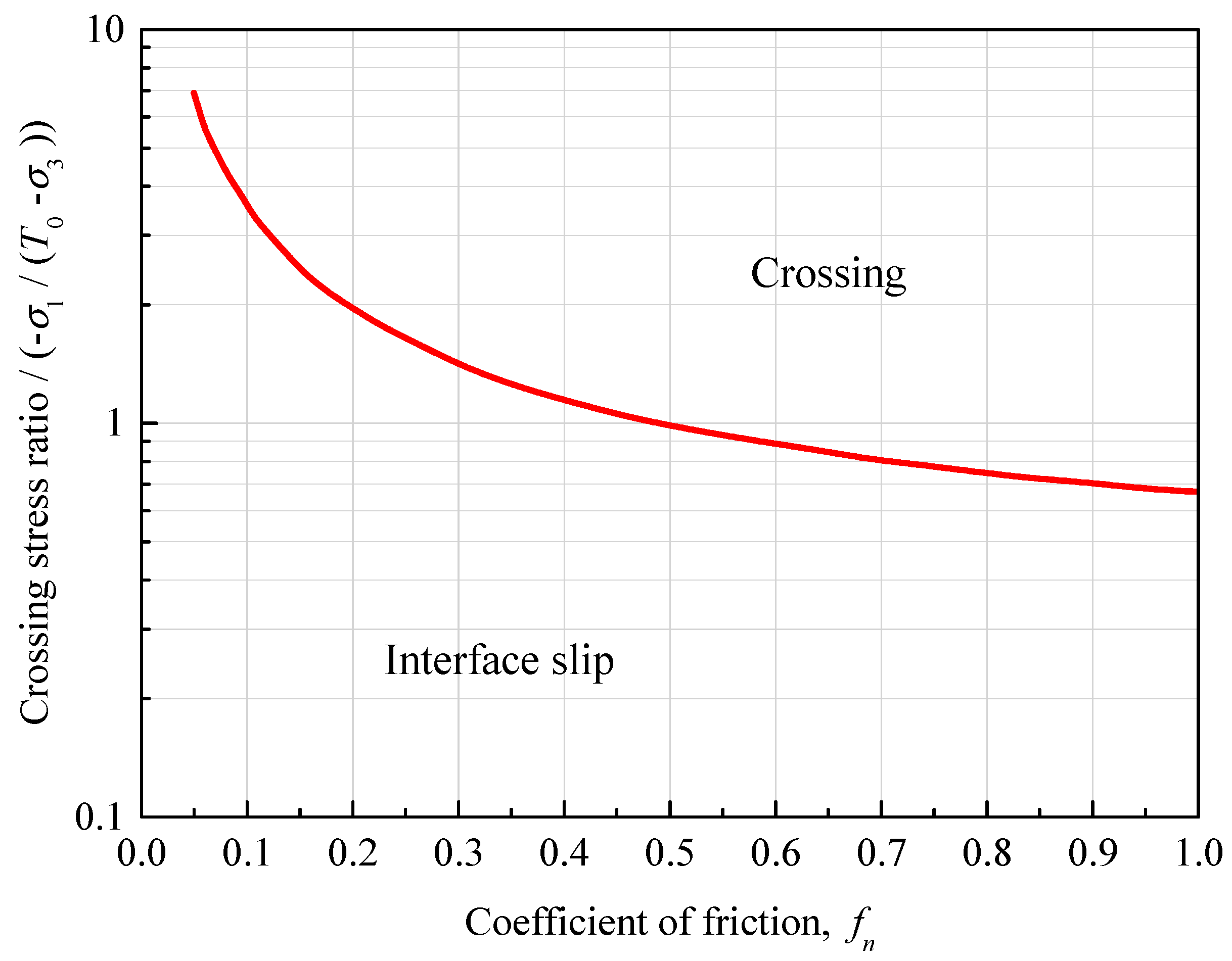
During the hydraulic fracturing process, fluid is injected into shale reservoirs through the wellbore. When the injection pressure exceeds the breakdown pressure, HF initiates around the wellbore and propagates to intersect with the NF. The prevailing conditions of the reservoir are instrumental to the interaction results between the NF and HF [17,18,19]. The first prevailing factor is stress ratio (i.e., the ratio of the maximum principal stress to the minimum principal stress). Another factor is the approaching angle—the angle between HF propagation orientation and the NF plane. Based on linear elastic fracture mechanics, Renshaw and Pollard [14] put forward a criterion for hydraulic fracture propagation across an orthogonal unbounded frictional interface. They demonstrated the relationship between the criterion they proposed and the friction coefficient to identify the crossing and no-crossing scenarios (Figure 1).
Gu and Weng [20,21] extended the criterion for non-orthogonal angles of the frictional interfaces with cohesion. We assumed that the interaction angle between the HF and the fault was the approaching angle β in Figure 2, which graphically illustrates the thresholds for different approaching angles under different stress ratios and friction coefficients. In addition, Gu and Weng [20] also stressed that the approaching angle played an important role in HF crossing NF.
Many physical experiments and numerical simulations have been conducted to understand the effect of rock reservoir properties on the interaction between the HF and NF, from which the following three conclusions can be drawn [22,23,24,25,26]: first, the increase of the approaching angle can improve the possibility of HF crossing NF due to the increasing difficulty for the fluid to flow into the NF when it is oriented closer to the normal direction of the HF propagation path. Second, the greater the stress ratio, the greater the possibility of the HF crossing the NF. It is easier for HF to propagate along the orientation of the maximum principal stress. The increase of stress ratio can make the reorientation of HF more difficult, which makes it easier for the NF to cross the HF. Third, the larger the friction coefficient, the greater the possibility of the HF crossing the NF. The increase in the friction coefficient makes deformation and shear behavior more difficult, which encourages HFs crossing NFs.
The fault activation and seismicity induced by the interactions between HFs and larger NFs (i.e., faults) was not fully understood in previous studies. However, fault activation and seismicity may result in severe problems, such as underground water pollution and land subsidence [27,28,29]. These problems are associated with the modification of shale reservoirs after hydraulic fracturing. Historically, there have been accidents caused by seismicity during hydraulic fracturing; for example, in Lancashire County, UK, two seismic events of Richter scale magnitude 2.3 and 1.5 were once observed during hydraulic fracturing, which resulted in the flow of injection fluid into the fault zone [30]. In addition, in Oklahoma, USA, a strong spatio-temporal correlation was found between the excitation time of hydraulic fracturing and 43 earthquakes (magnitudes ranging from 1.0 to 2.8) [31]. Each case of felt seismicity, as well as one recently reported case of larger than usual events in Ohio, [32] have all been associated with the activation of faults.
Field data from thousands of hydraulic fracturing stimulation operations have revealed that seismic events could extend hundreds of meters upwards in the areas 900–4300 m underground [33]. Generally, the induction of seismic events is associated with fault activation [10], and although many data show that hydraulic fracturing can result in fault activation and seismicity, there are many problems and uncertainties that need to be addressed with quantitative solutions. The qualitative analysis of the effect of the injection site in fault activation and seismicity has rarely been observed in previous data reports and research studies.
In this study, a coupled hydro-mechanical model and the moment tensor method were used to evaluate the magnitude and affected area of injection-induced seismic events. The micro-parameters of the proposed model were calibrated with analytical solutions of the interactions between HF and the fault. A series of numerical simulations were performed to investigate the effect of the injection site on fault activation and seismicity. Based on the simulation results, the shale reservoir after fracturing treatment was divided into five zones to investigate the optimal distance between the injection hole and the fault.
2. Numerical Simulation Procedure
2.1. Coupled Hydro-Mechanical Model
The Particle Flow Code (PFC), a two-dimensional numerical program based on the discrete element method (DEM), was used for the simulations. In this model, the shale reservoir is discretized into many circular particles bonded together. The parallel bond model was selected to bond particles, given that the simulation of a shale reservoir with this model is much closer to reality [34]. The fault is represented by the smooth joint (SJ) model where it is composed of two parallel and overlapping planes. In a shale matrix, particle contacts can result in crack initiation in any orientation. When a SJ is assigned to contacts between particles, these contacts are removed and the new contacts can only move along the orientations of the identified SJ, regardless of the original contact orientations. With these PFC features, it was well-suited to achieve the objectives of the present study.
Figure 3 is the enlarged view of the coupled hydro-mechanical model, and demonstrates fluid domain, true pore space, and flow channel. In this figure, fluid domain is defined by the polygon surrounded by the particle centers. True pore space is represented by the geometric space left after particle bonding. Pores are interconnected, and so form a pore network. Fluid flow in the pore network is modeled by the flow channels at the particle contacts that have hydraulic apertures.
The volumetric flow rate per unit width in pore Q is modeled by the Cubic law [35]:
where a is hydraulic aperture; μ is fluid dynamic viscosity; PA − PB is the fluid pressure difference between the two neighboring pore spaces; and L is flow channel length.
Hydraulic aperture a can be defined by an equation associated with the normal stress of particle contacts σn [36]:
where azeo and ainf are aperture values at zero and infinite σn, respectively; and coefficient is the speed of aperture decay with increasing σn ( usually selects 0.15 after [36]).
The increment of fluid pressure ΔP in pore within each time step Δt can be calculated with Equation (3) [37]:
where Kf is fluid bulk modulus; Vd is pore volume; and ΔVd is increment of pore volume.
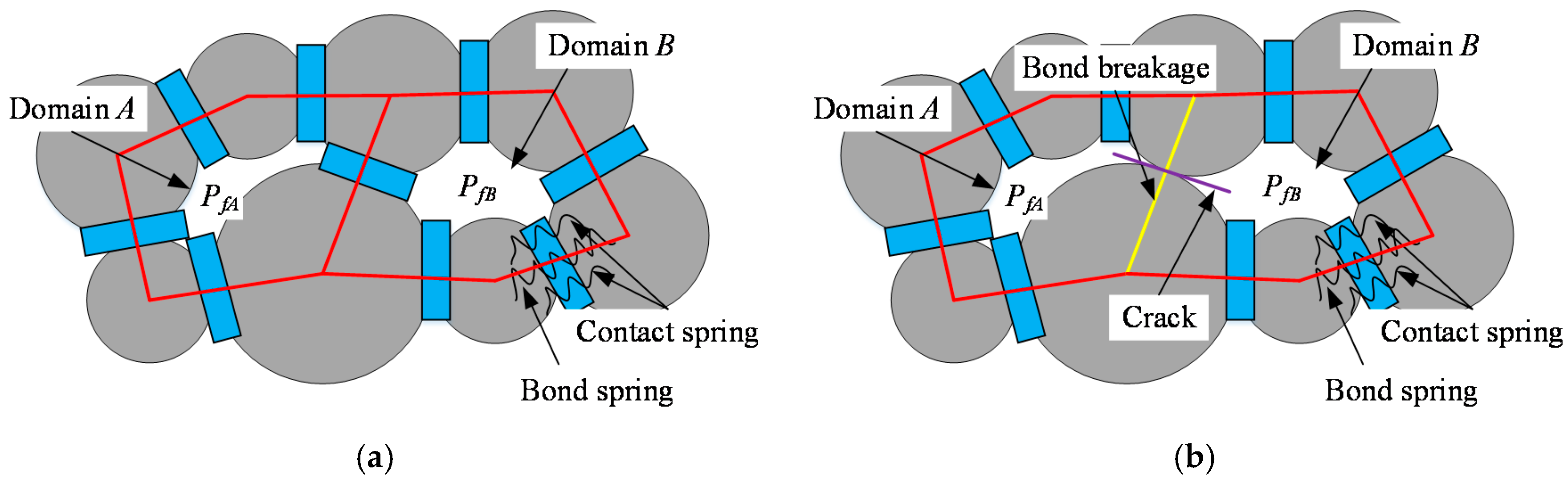
Fluid pressure can result in particle deformation that in turn changes the stress states and apertures of the flow channels. The increase of fluid volume and pressure resulting from the fluid injection will break the contacts between the particles. Once a parallel bond is broken, the fracture aperture is set to the aperture at zero normal stress. The pressure value in the emerged domain equals the mean value of the pressure values in previous two domains (Figure 4). In this case, the changed fluid pressure can be calculated with the following equation:
where and are the fluid pressure related to Domain A and Domain B, respectively, in Figure 4.
However, this equation is not applicable when there is a large difference between the volumes of the two domains. Therefore, the fluid pressures in the two domains can be calculated with Equation (5) in the case of fracture initiation:
where VfA and VfB are the volume of fluid existing in Domain A and Domain B, respectively, in Figure 4. V0A and V0B are the volume of Domain A and Domain B, respectively, under 0 MPa hydraulic pressure.
2.2. Moment Tensor Method
On a laboratory scale, the acoustic emission (AE) signal is generated with the initiation of new cracks resulting from particle contact breakages [38]. On a field scale, many similarities have been observed between seismicity and AE signal such as, the path of crack propagation and energy release. However, the frequency of seismic wave is different from that of the AE signal [39]. Seismic wave amplitude can be calculated with the moment tensor method. In numerical simulation, if every single fault slip or contact breakage is regarded as a seismic event, the magnitudes of all seismic events are essentially similar, which is not consistent with reality.
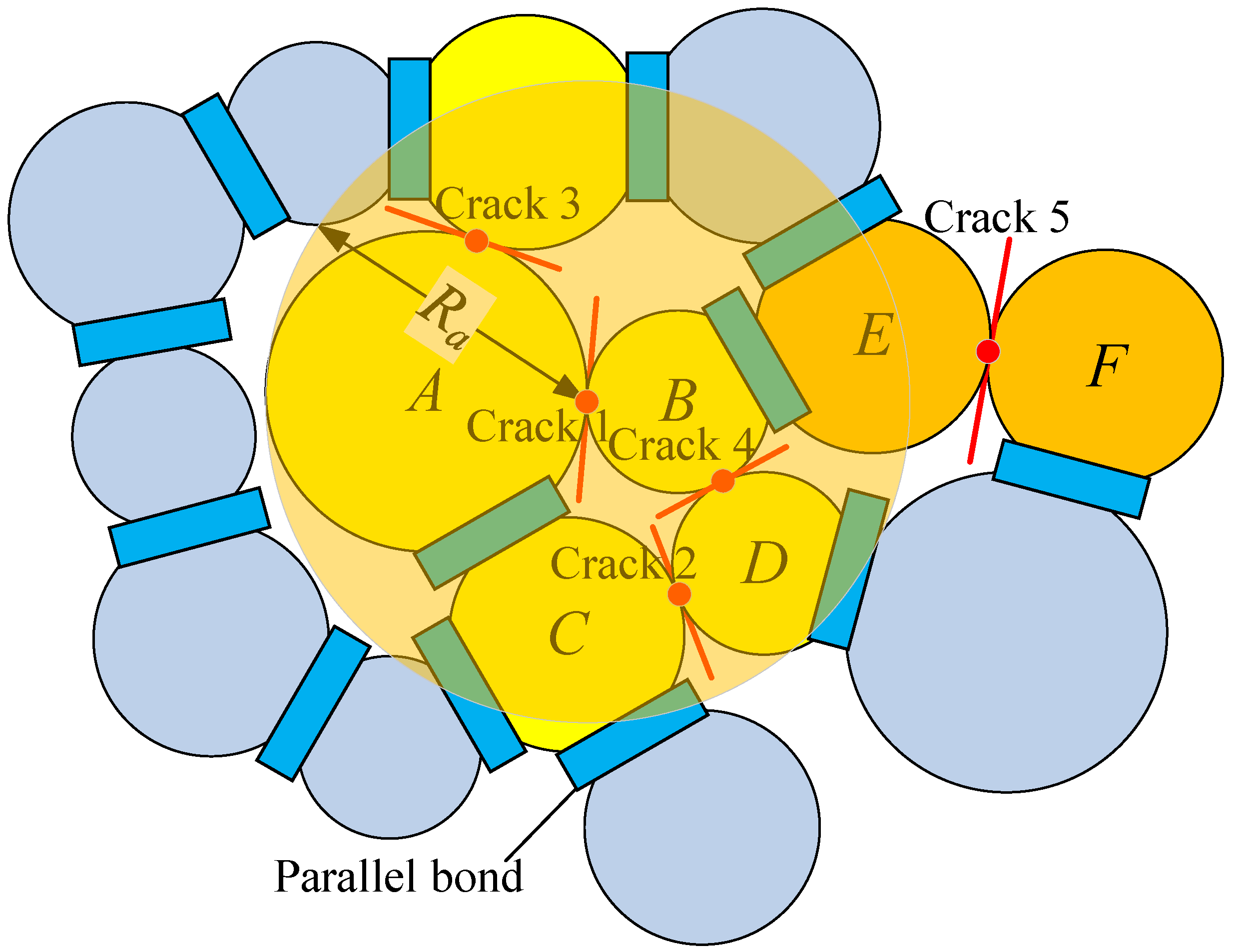
When crack initiation is induced by fault slip or contact breakage, the particles at two ends of the new crack are defined as source particles (Particle A and Particle B). Only the cracks induced by the contact breakages with source particles may belong to the same seismic event (Figure 5). In the coupled hydro-mechanical model, the increments of the force and force moment resulting from the initiation of new cracks can be transmitted via particle contacts. Therefore, the magnitude and affected areas of a seismic event will also increase with the transmission of the force and force moment.
Definition of the excitation time of the same seismic event is demonstrated in Figure 6. The time that Crack 1 takes to propagate to the border of its affected area was defined as Excitation time 1 (T1). Therefore, the moment tensor updates within each time step within T1. If there is no initiation of new cracks within T1 or affected area of Crack 1, the seismic event only includes one crack and its total excitation time is T1. If Crack 2 initiates within T1 and the affected area of Crack 1, the overall affected area of this seismic event becomes the sum of the affected areas of Crack 1 and Crack 2. If the time that Crack 2 takes to propagate to the border of its affected area is defined as Excitation time 2 (T2), the overall excitation time of this seismic event is T0 (Figure 6).
Similarly, if Crack 3 initiates within T0 and the sum of the affected areas of Crack 1 and Crack 2, the affected area of this seismic event is the total affected areas of Crack 1, Crack 2, and Crack 3 (Figure 5), and its total excitation time is T0 (Figure 6). Crack 4 and Crack 1 are not included in the same seismic event because Crack 4 initiates after T0, though it is still within the affected area of Crack 1. Additionally, Cracks 5 and 1 do not belong to the same seismic event because Crack 5 is not within the affected area of Crack 1, though it initiates within T0.
In the proposed model, the force and force moment resulting from the particle movement can be obtained directly. Therefore, the moment tensor in the case of crack initiation can be calculated with Equation (6):
where Mij is the scalar seismic moment in the calculation; and ΔFi and Lj are the nth component of the contact force and the corresponding arm of the force.
Then, the maximum scalar moment of the moment tensor M0 can be calculated with Equation (7):
3. Model Steps and Validation
3.1. Model Steps
The set of in-situ stresses in this study were cited from the shale gas reservoirs in Apalachee, Pennsylvania, USA [40]. The locations of the specific reservoirs and Marcellus shale distribution are illustrated in Figure 7. It reveals that most reservoirs are in Pennsylvania and West Virginia, where Marcellus shale rocks have a depth (z) = 2000–2500 m. The maximum and minimum principal stresses (SH and Sh) can be calculated with Equations (9) and (10), respectively [41]:
where z is depth. Here, the depth z is 2.25 km.
A 160 m × 100 m model and a pre-existing fault was generated in PFC. Figure 8 demonstrates the geometry and boundary conditions of the model. To monitor the effect of the injection site on fault activation and seismicity accurately, only the area of interest (left area of the figure, containing a fault) was analyzed in the following. The wellbore was located at the very center of the model to mitigate the boundary effect. The initiation, propagation, and coalescence in the left half of the model was closely monitored. The maximum and minimum principal stresses were loaded in horizontal and vertical orientations, respectively; however, it should be noted that depending on the level of stress anisotropy, HF initiation from a wellbore could form a complex geometry.
The parameters of particle contact were selected to represent the properties of the rock matrix and the fault in the reservoir. For the parameters of the fault in the proposed model, both the tensile strength and cohesion were assigned as zero to ensure consistency with the graphical illustration of the threshold curves [20]. The anisotropy of the stress was represented by stress ratio. The interaction angle between HF and the fault was called the approaching angle (β). In this study, β was assigned as 75°. The distance between the injection hole and the fault was named as Lif, which was assigned as 10, 20, 30, 40, 50, and 60 m, respectively.
3.2. Model Validation
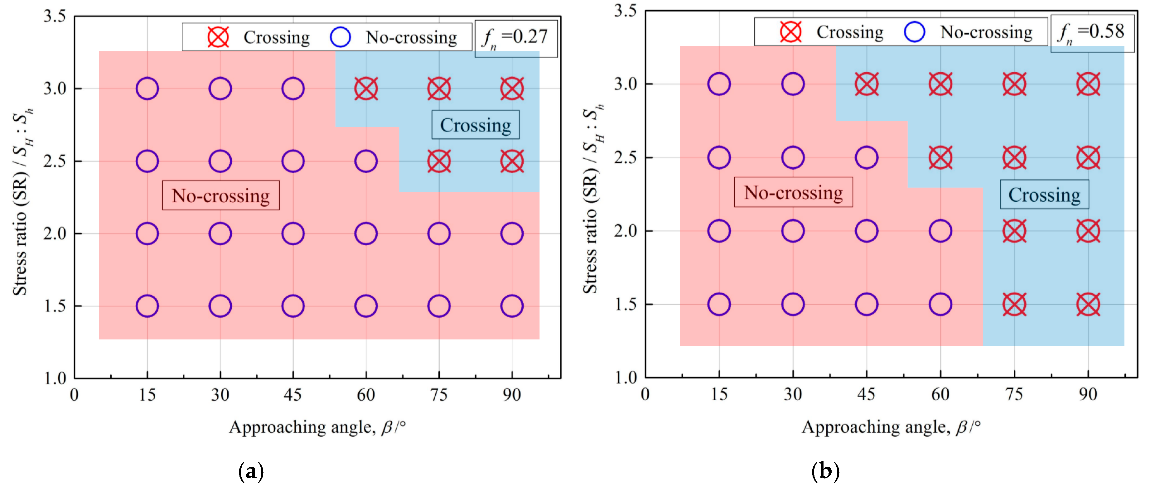
The accuracy of the proposed model in simulating interaction behaviors between HF and the fault was demonstrated by examining the HF propagation trajectory in an isotropic shale reservoir. The results were then compared with published analytical solutions [20]. Figure 9 presents the comparison results between the numerical simulations and analytical solutions under different friction coefficients, fn, and approaching angles, β. Both the numerical simulations and analytical solutions revealed that an increase in approaching angle, stress ratio, and friction coefficient could increase the possibility of HF crossing the fault. Figure 10 shows that in most cases, the interactions between HF and the fault obtained from the numerical simulation were consistent with those obtained from the analytical solutions. The parameters of the shale matrix and fault characteristics of the validated model are listed in Table 1.
The initial and infinite hydraulic apertures were first calculated based on the empirical values in the literature [36], then their final values were determined using the trial and error method. These apertures were assigned to rock matrix (represented by parallel bond, PB) and SJ. In the author’s previous work described in Reference [43], different apertures were assigned to PB and SJ, and a sensitivity analysis was made on the apertures. The results showed that the assignment of different apertures to PB and SJ had a very limited impact on the simulation results. Therefore, for the sake of convenience, the same aperture was assigned to both PB and SJ.
Yoon [36] set the dilation angle to 3° when simulating the fault, while Wang [44] set this value to 0°. A sensitivity analysis was conducted on the parameters of SJ, which found that the dilation angle within the range of 0–5° had a very small effect on the simulation results. As a result, the default value (0°) was selected in the simulation.
The numerical simulation results were inconsistent with the analytical analysis in three cases: Case 1 (β = 60°, fn = 0.65); Case 2 (β = 60°, fn = 0.85); and Case 3 (β = 45°, fn = 0.85). There are two possible reasons for these discrepancies. First, in the case of small stress ratio, instantaneous stress changes occurred around the HF–fault interaction area. Second, the same parameters with analytical solutions were assigned for the tensile strength and cohesion of the fault in the model validation, which was not applicable in a real numerical simulation. Therefore, the parameters of the fault are in need of further validation. Nevertheless, despite the minor disagreements, the results of the numerical model displayed a remarkable consistency with the analytical solutions.
In contrast to the zero tensile strength and cohesion used for the fault, the fault properties listed in Table 2 were again assigned for the proposed models to simulate the fault in a more realistic way. The parameters of the rock matrix and fluid properties, as well as the operational conditions remained unchanged. The numerical simulation of the further model validation was performed under four different stress ratios (1.5, 2.0, 2.5, and 3.0), six different approaching angles (15°, 30°, 45°, 60°, 75°, and 90°) and two different friction coefficients (0.27 and 0.58).
The numerical simulation results of the further model validation are illustrated in Figure 10. They reveal that the greater the stress ratio, approaching angle, and friction coefficient, the higher the possibility of HF crossing the fault, which is consistent with the results of the physical experiment (numerical simulation) in Section 1 [22,23,24,25,26]. The final calibrated micro-parameters of the fault after further model validation is listed in Table 2.
4. Results and Analysis
To investigate the effect of injection site on fault activation and seismicity during hydraulic fracturing, comparative analyses such as fault slip, injection pressure distribution, and magnitudes of seismic events were conducted based on the calibrated model in Section 3.
4.1. Fault Slip Displacement
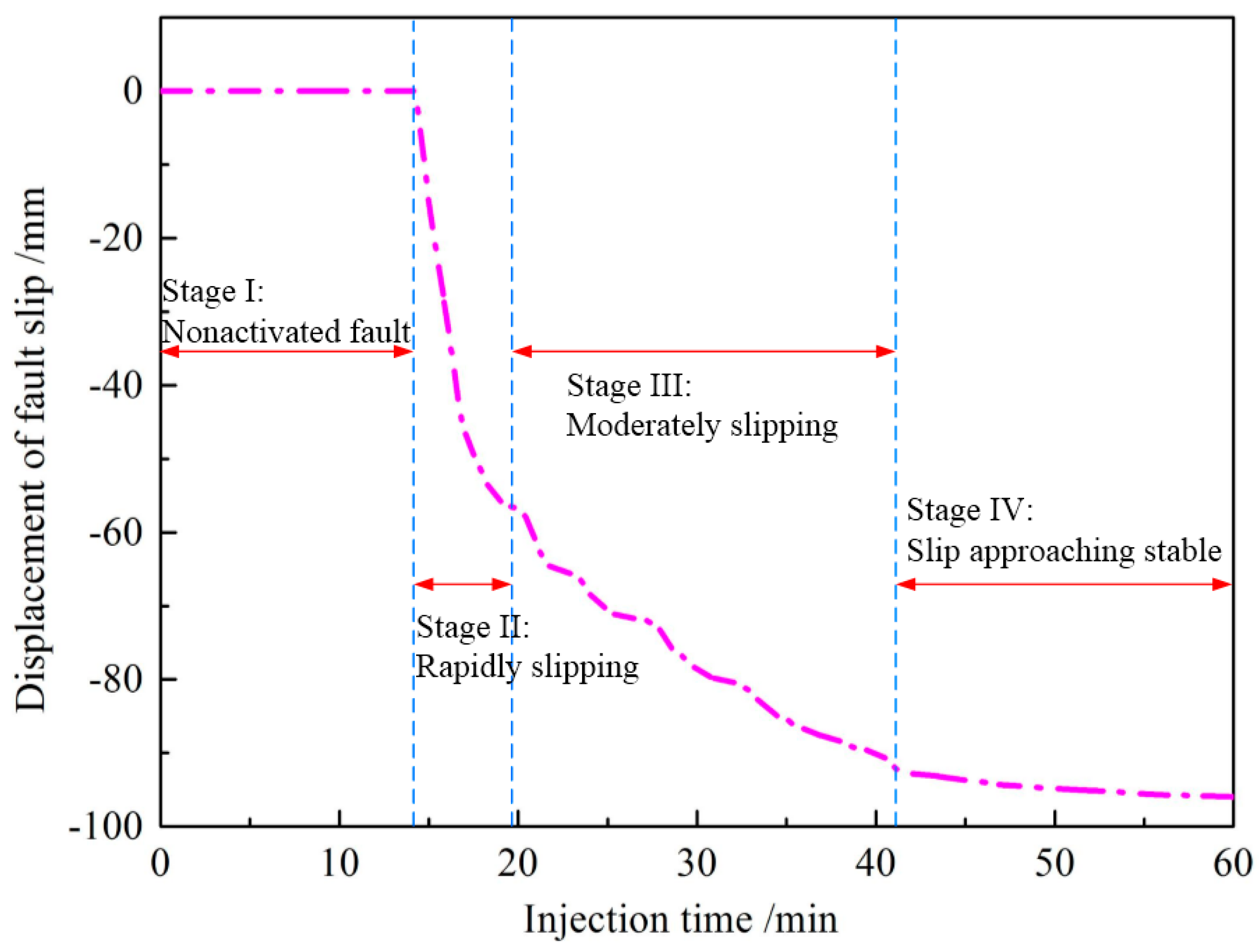
Fault slip displacement is one of the key factors in quantitatively evaluating the effect on fault activation. Figure 11 illustrates the representative curve of injection-induced fault slip. When monitoring the fault slip, a measurement region was arranged with a radius of 5 m at three locations in the middle of the fault, respectively. Each measurement region contains a number of SJs. As the horizontal and vertical displacements in each time step were recorded by means of the measurement region, the fault slip distance was ultimately obtained through the average of the three measurement regions (Figure 8).
The curve can be divided into four stages according to injection time and fault slip rate: the non-activated fault stage (Stage I), the rapidly slipping stage (Stage II), the moderately slipping stage (Stage III), and the slip approaching stable stage (Stage IV).
Stage I: As there was a certain distance between the injection hole and the fault, the HFN and the fault did not interact with each other and the fault slip displacement remained almost unchanged. Stage II: Before fault activation, the shale reservoir around the fault was in a state of unbalanced stability. However, once the stress disturbance occurred around the shale reservoir (i.e., the HFN moved close to the fault), the fault would be activated immediately. Stage II lasted for a short time, but had the most significant effect on fault activation. Stage III: After the rapid slip stage, the shale reservoir around the fault entered into a new stable state and the fault continued to slip with a slip rate obviously smaller than that in Stage II. Stage III was the transition stage of the fault from activation to a stable state. Stage IV was the final stage of the fault activation induced by hydraulic fracturing, where the stress in the shale reservoir restored its balance.
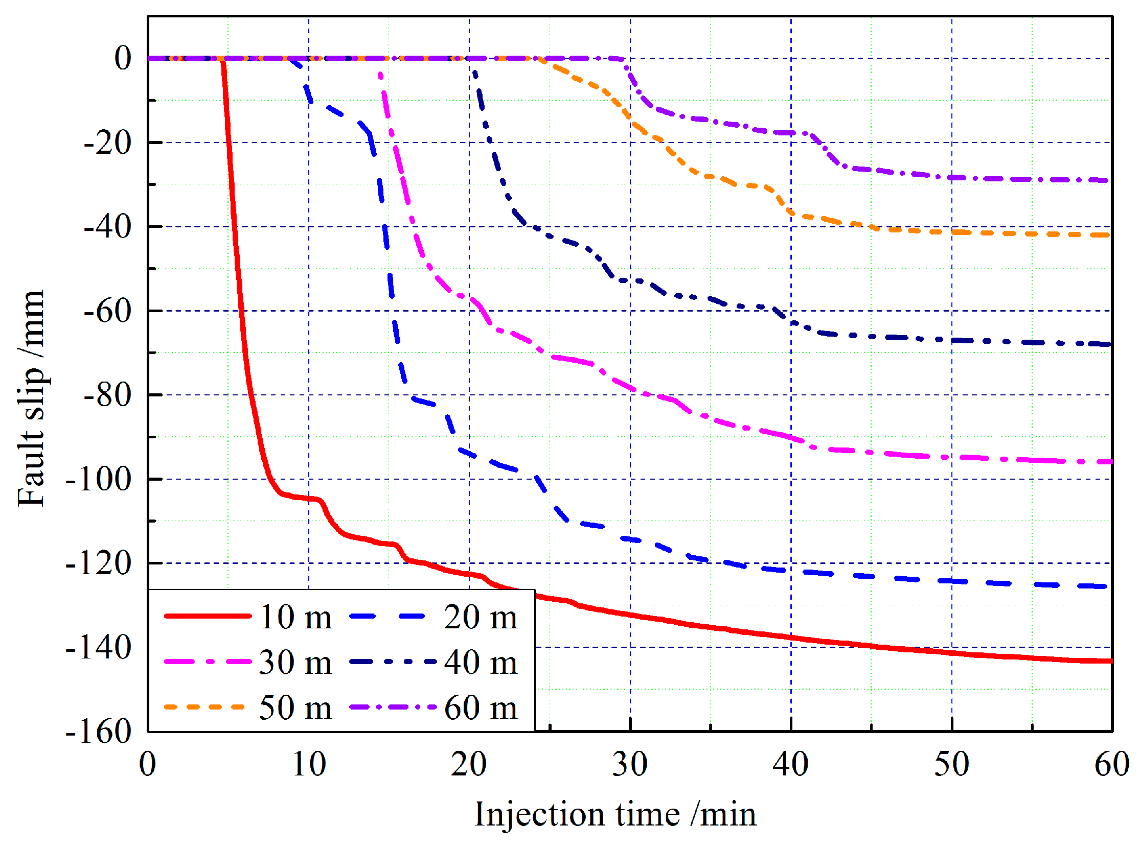
Figure 12 and Table 3 show the duration time and fault slip displacement at four stages when Lif ranged from 10–60 m. These revealed that duration presented a linear increase with the increase of Lif in Stage I. In Stage II, although the durations of all injections were shorter than 10 min, the injection pressure at this stage had the most significant effect on the fault slip displacement. In Stage II, the minimum Lif (Lif = 10 m) resulted in the most serious slip (more than 100 mm) while the maximum distance (Lif = 60 m) only brought about 15.13 mm. In this stage, the fault slip displacement presented a negative exponential distribution with the increase of Lif.
In Stage III, the time for the fault to restore its stability was the longest (>30 min) at Lif = 10 m due to the most severe stress disturbance. Although the minimum distance (Lif = 10 m) also resulted in the longest displacement in Stage III, the gap between Lif = 10 m and those of the other distances was much smaller. In Stage IV, the fault was restored as stable again with the slip displacement remaining almost the same regardless of the changes of Lif.
4.2. The Normalized Range of Fault Activation
Figure 13 illustrates the effect of the injection site on the range of fault activation. Due to the difference of the pre-existing fault length in the model under different approaching angles, the y-axis was set as the normalized range of fault activation Rn in Figure 13, which was identified as:
where Ra and Rl are the activated and total lengths of the fault.
This revealed that all normalized ranges of fault activation under different approaching angles were above 70% when the injection hole was relatively near to the fault (Lif = 10 or 20 m). At Lif = 40 m, the normalized range of fault activation was approximately above 70% when β = 30°, but dropped to below than 15% when β = 90°. However, the difference between the normalized range under different approaching angles varied little when the injection hole was relatively far away from the fault (Lif = 60 m). In particular, although both the approaching angle and Lif can influence the range of fault activation, the range of fault activation is more sensitive to the latter.
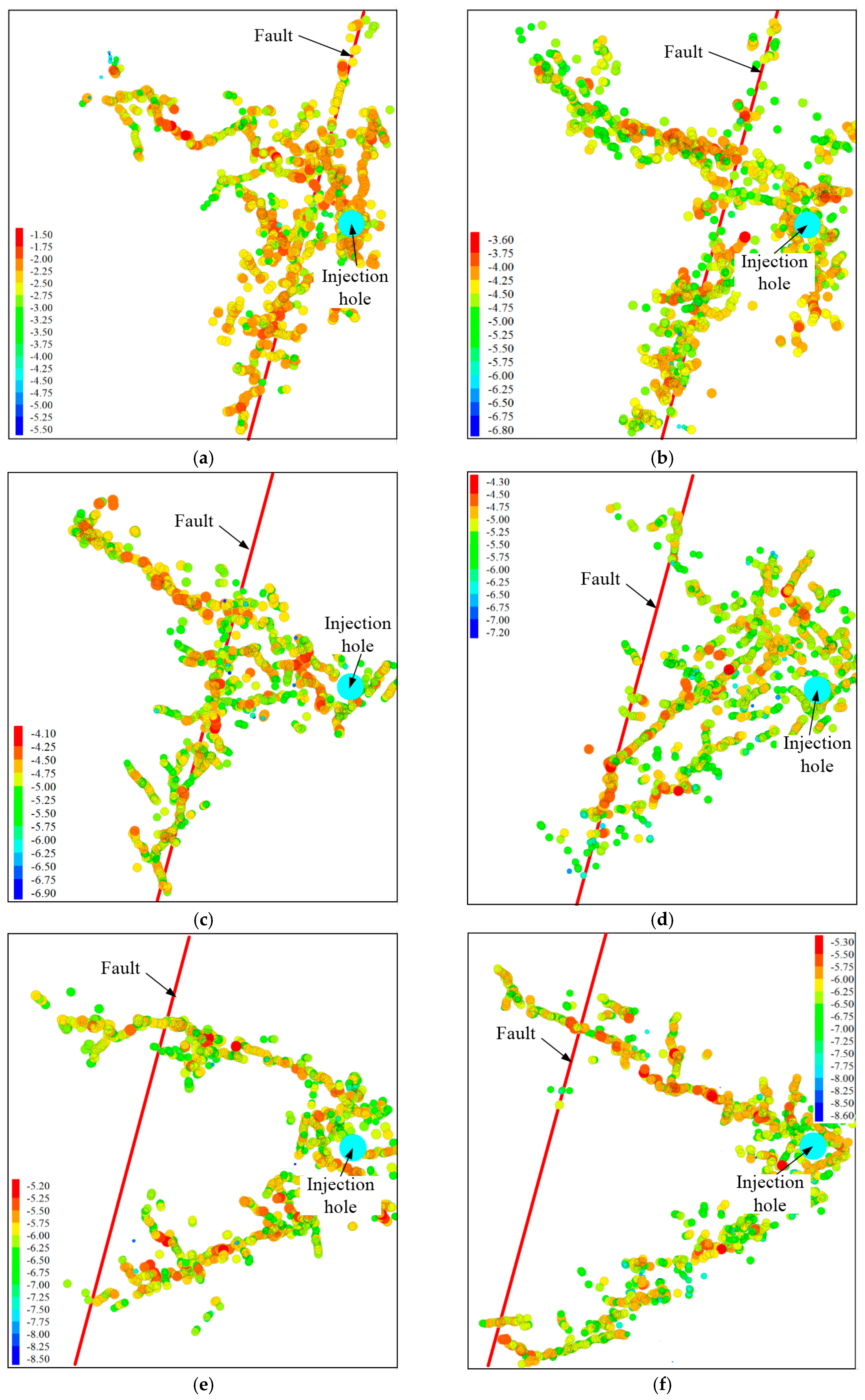
The seismic events induced by fault slips and contact breakages with variation of Lif during hydraulic fracturing are illustrated in Figure 14. In this figure, different magnitudes of seismic events are represented by different colors. When Lif was 10 or 20 m, HFs were initiated in the shale reservoir around the injection hole due to the short distance between the injection hole and the fault (Figure 14a,b). The fault was activated rapidly after the initiation of the HFs. In addition, the activated fault resulted in continuous stress disturbance to the shale reservoir around the injection hole. Meanwhile, the stress disturbance induced by the fractured zone around the injection hole led to further fault slip and expansion of the activation range. The magnitude of the seismic events increased gradually during this interaction process, which resulted in the maximum range of the fault activation within this distance.
With the increase of Lif (Lif = 30 or 40 m), the interaction between the stress disturbance induced by fluid injection and fault activation became much less obvious, and the magnitude of seismic events also decreased. Furthermore, the normalized range of fault activation fell to below 60%, even 28.68%, when Lif = 40 m (Figure 14c,d). When there was a large distance (Lif = 50 or 60 m) between the injection hole and the fault, the stress disturbance induced by fluid injection could barely activate the fault, and almost all seismic events were caused by the HFN. In addition, the magnitudes of these seismic events were almost the same as the magnitudes without the fault. In Figure 14e,f, the fractured rock zone was only formed within 15 m of the injection hole. Within this distance, instead of interacting with each other, the injection pressure and fault slip formed several clear HFNs which propagated along the orientation of the principal stress.
4.3. Injection Pressure Distribution
Figure 15 illustrates the distribution of the injection pressure in different Lif cases. When the fluid injection began, particle contact breakage around the injection hole was observed and injection pressure distribution was essentially similar in all Lif conditions. At this stage, the distribution of injection pressure was not directly associated with the injection site or the orientation of the maximum principal stress. Because SH > Sh, cracks propagated in the orientation of SH and injection pressure gradually increased with continuous fluid injection. When Lif = 10 m, the HFN first started to interact with the fault. At this moment, the injection pressure was still unstable. Therefore, the HFN propagated in an orientation perpendicular to that of the fault after it interacted with the fault. With the increase of Lif, although HFN still propagated in an orientation perpendicular to that of the fault, the HFNs that propagated in other orientations decreased when Lif = 20, 30, or 40 m, and finally totally disappeared (Lif = 50 or 60 m). The magnitudes of the injection pressures were almost the same under different Lif conditions due to the same injection rates, properties, and boundary conditions of the rock reservoir.
4.4. Cumulative Frequency of Seismic Events
It is well-known that the magnitude of seismic events follows a power-law distribution. Therefore, a Gutenberg–Richter-type relationship was used to examine the magnitudes of the seismic events [43]:
This relationship equation has been widely used to investigate seismic events in physical experiments or field tests. Parameter a refers to the mean activity level in the region investigated, and parameter b refers to the proportion of small events in comparison with large events. The smaller the b-value, the larger the proportion of great seismic events, and vice versa.
To investigate the cumulative frequency of seismic events induced by hydraulic fracturing, the curves representing the relationship between magnitudes and logarithmic frequency of seismic events are fitted in Figure 16. The cumulative frequency of seismic events follows a linear distribution where the magnitude of seismic events is relatively larger, which is consistent with the results obtained in References [45,46,47]. Table 4 shows the fitting of a- and b-values of cumulative seismic events when Lif ranged from 10 to 60 m. The b-values were calculated using the least square method. Since seismic events cannot form a straight line, serious deviations are caused if all the points on the curve are taken into account. Hence, only the straight-line regions were fitted.
This revealed that the b-value increased with distances far away from the injection hole, meaning a decrease in the frequency of seismic events with large magnitudes. The injection-induced seismic events were highly sensitive to the change of injection site. When Lif was longer than 50 m, the magnitudes of injection-induced seismic events tended to be small and stable.
4.5. Magnitude Distribution of Seismic Events
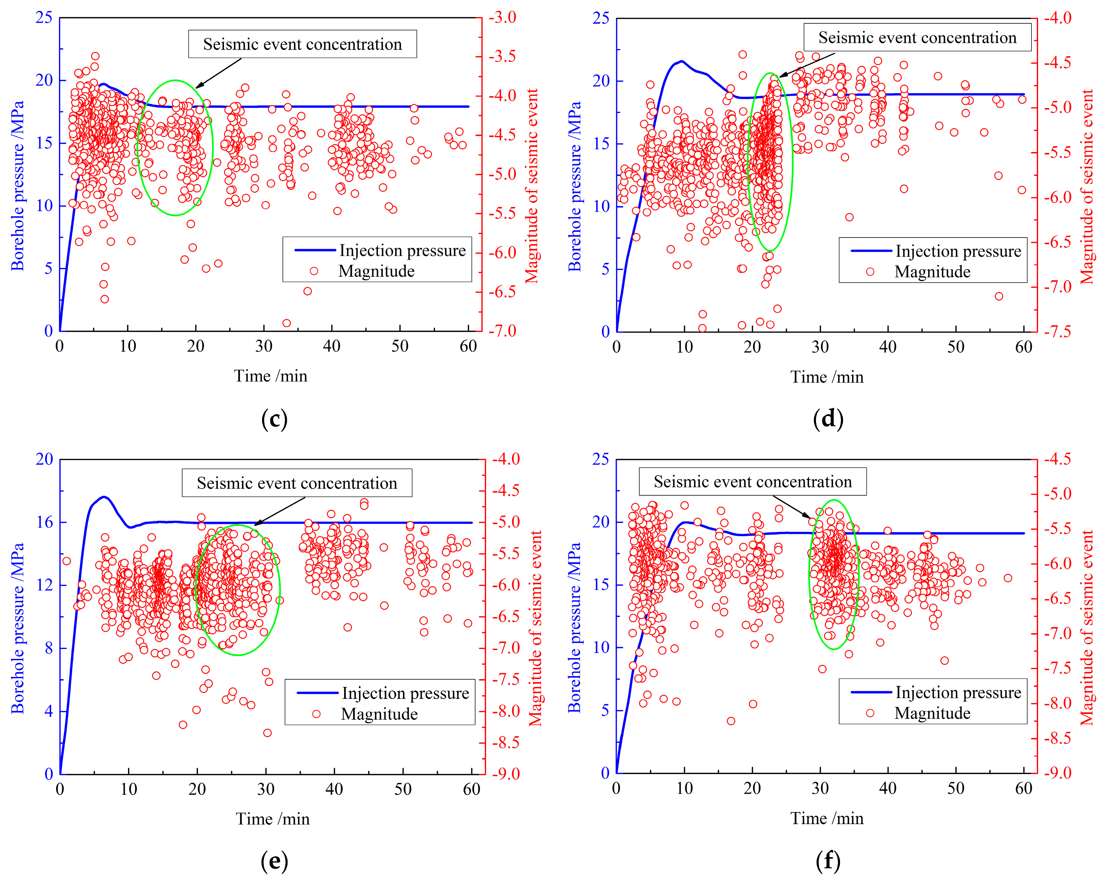
The frequency of the injection-induced seismic events with different magnitudes is also a key effect factor. Figure 17 illustrates the distributions of borehole pressure and injection-induced seismic events after fluid injection. Figure 18 demonstrates the relationship between the magnitude and frequency of the injection-induced seismic events. In Figure 18, the frequency of seismic events exhibits a normal distribution across different magnitude intervals.
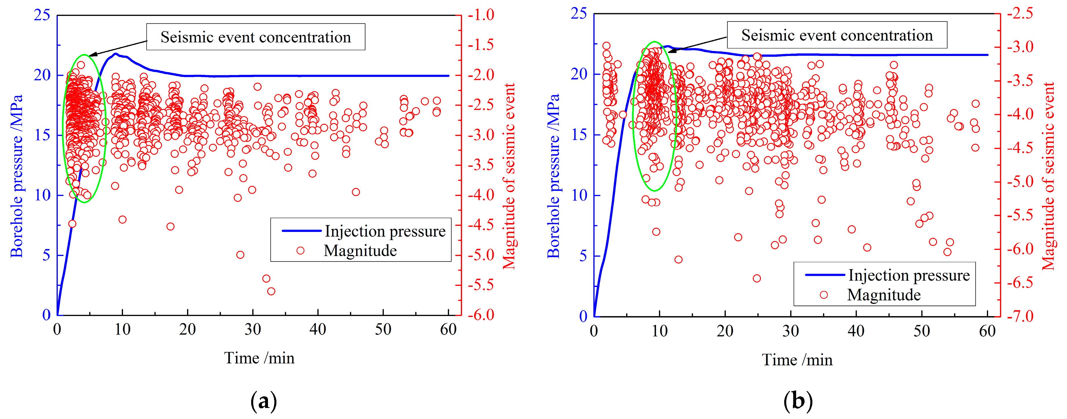
Most of the seismic events were induced at the very beginning of the injection, and the magnitudes of these seismic events ranged from –3.5 to –1.5 at Lif = 10 m (Figure 18a). During the whole injection process, both the highest frequency and the largest magnitudes of the seismic events were concentrated within the first eight minutes, as the fault was activated soon after the beginning of the fluid injection. This concentration of seismic events was the result of the interaction between injection-induced stress disturbance and fault slip (Figure 17a). When the injection time exceeded 20 min, the borehole pressure gradually stabilized, resulting in a decrease in the injection-induced seismic events.
When Lif increased to 20 or 30 m, the particle contacts were broken by injection pressure which disturbed the shale reservoir around the injection hole to generate a handful of seismic events. In this case, more than 80% of seismic events (M = –5.5 to –3.5) also appeared in the HFN–fault interaction period (Figure 17b,c). Similarly, the frequency of the seismic events induced by fault slips decreased gradually with the increase of injection time (Figure 17b,c). With the increase in distance between the injection hole and the fault, seismic event concentration also appeared in later periods.
Seismic event concentration appeared at 20 min after the beginning of the injection when Lif = 40 m (Figure 17d) and the magnitudes of the injection-induced seismic events mainly ranged from –6.5 to –4.75 (Figure 18d). In the case of the longest distance between the injection hole and the fault (Lif = 50 or 60 m), seismic event concentration also appeared later than in all other Lif scenarios and the magnitudes of the injection-induced seismic events (M = –7.0 to –5.5) were also much smaller than other Lif cases (Figure 14f and Figure 18e).
The seismic event concentration is a result of the fault slip and contact breakages caused by the interaction between HFN and the fault. Seismic events that occur before concentration are caused by the injection-induced initiation of cracks in the rock reservoir, while those that appear after concentration are mainly induced by fault slip. When Lif was relatively short, the duration of the fault slip was long, which made the restoration of the stress balance in the fault more difficult. The frequency of the seismic events induced by the fault slip was higher than that of the seismic events induced by particle contact breakage. In particular, the borehole pressure determined by the injection rate, properties of the rock reservoir, and other external conditions varied from 18–22 MPa all the time, regardless of the changes of Lif.
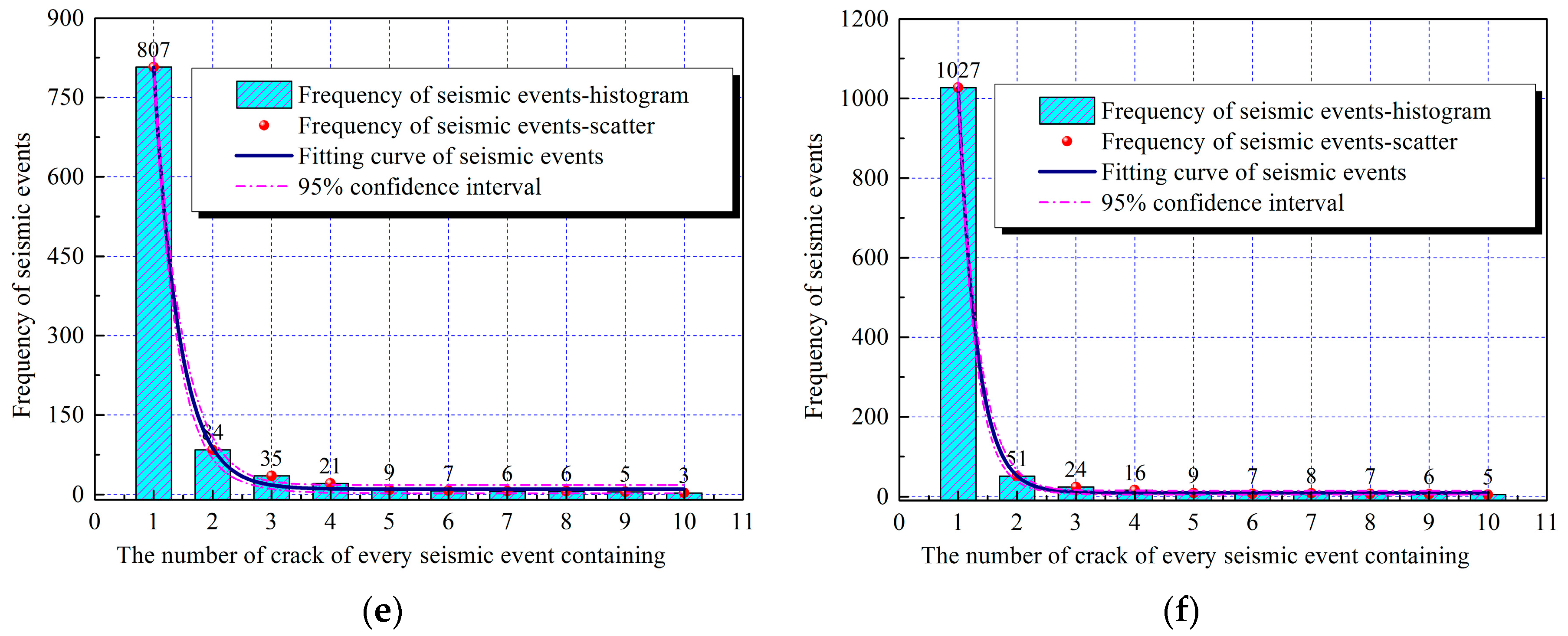
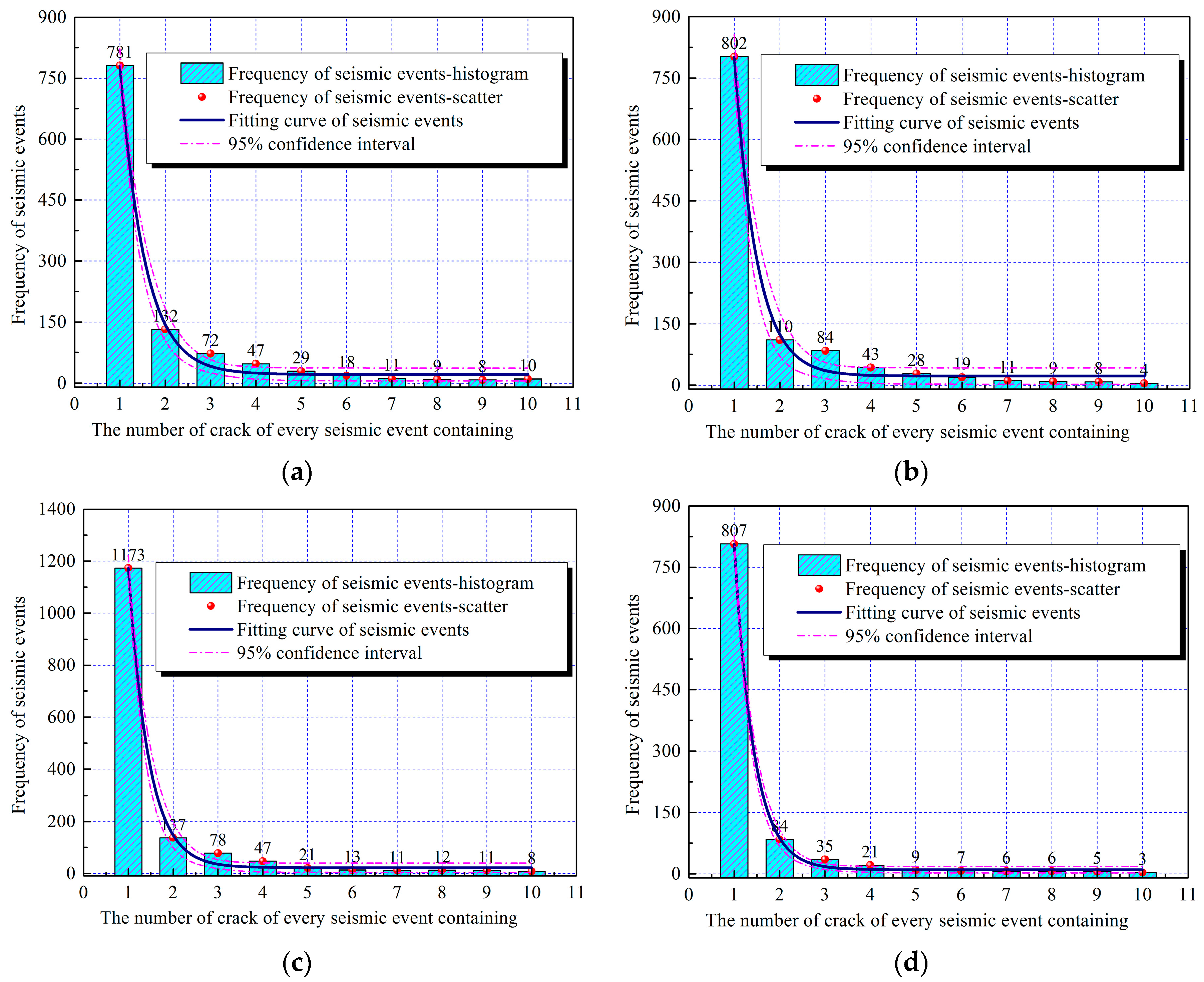
4.6. Seismic Events Containing the Crack Number
According to the definition of seismic event (Section 2.2), every seismic event may contain one or more cracks. Figure 19 illustrates the relationship between the number of cracks contained by each seismic event (x-coordinate) and the frequency of the seismic events (y-coordinate), and revealed a negative exponential relationship between the two, which meant that the frequency of a seismic event decreased rapidly with an increase in the crack number contained in seismic events. When Lif = 10 m, the frequency of the seismic events containing one crack accounted for 66.24% of the total frequency of only the seismic event, and the frequency of the seismic events containing 10 or more cracks reached 62 (Figure 19a). The frequency of the seismic events containing one crack grew gradually with an increase in the distance between the injection hole and the fault. It accounted for more than 80% of the total seismic events when Lif = 40 m (Figure 19d). The frequency increase of the seismic events containing one crack meant a decrease in the frequencies of large-magnitude seismic events, since more of the cracks were contained by a seismic event, given the larger the magnitude and affected area of the seismic event. Therefore, seismic events resulted in the maximum activation of the fault and the severest damage to the wellbore when Lif = 10 m.
5. Discussion
In Section 4.1, the measurement circles were applied to monitor the fault slip. Frankly speaking, there is some error in the setting of these measurement circles. In DEM, particles are bonded by contact, so the stress and displacement obtained are the results measured in one particle or in a region. Although finite element method (FEM) has an advantage in this respect, it has many drawbacks in initiation and propagation processes of simulated cracks. The presence of a crack is likely to affect the measurement of stress or displacement, but the error can be reduced by measuring slip displacement of the fault with sufficient measurement circles.
In addition, the b-value can be determined through both least square method and maximum likelihood method. Although different methods can yield somewhat different b-values, the conclusions they draw are consistent. That is, the shorter the distance between the fault and the injection location, the smaller the b-value obtained, and thus the greater the magnitude of seismic event. We will discuss in future work as to which b-value determination method agrees better with reality.
6. Conclusions
During hydraulic fracturing, fault activation and seismicity may result in underground water pollution and land subsidence. In this paper, a large quantity of numerical modeling was performed using a coupled hydro-mechanical model in PFC to investigate the effects of injection site on fault activation and seismicity during hydraulic fracturing. Analytical analyses with six key factors were conducted to investigate the numerical simulation results. From the analysis, the following conclusions were drawn:
- (1)
- The fault slip displacement and activation range increased at first, and then remained stable with an increase in the distance between the injection hole and the fault. In addition, there is a critical distance and interaction between the injection-induced stress disturbance, and fault slip was gentle when the actual distance between the injection hole and fault was larger than the threshold distance.
- (2)
- There was a linear relationship between the magnitude and the logarithmic frequency of the seismic events in a concentration zone. The b-value decreased with the increase in the distance between the injection hole and the fault. When Lif was relatively large (Lif ≥ 50 m), the b-value declined by more than 50%, which meant that no large-magnitude seismic event and affected area was generated within this distance range.
- (3)
- Seismic event frequency presented a normal distribution within the different magnitude ranges, and a negative exponential distribution was observed between the crack number contained in the seismic events and the seismic event frequency. In the case of the shortest Lif (Lif = 10 m), seismic event magnitudes concentrated in ranges from –3.5 to –1.5. In addition, the frequency of seismic events containing one crack was the lowest, while that of the seismic events containing more than 10 cracks was highest.
- (4)
- The injection rate, properties of the rock reservoir, and boundary conditions remained unchanged, resulting in small variations in the magnitude of borehole pressure (18–22 MPa). However, the distribution of injection pressure was quite sensitive to the change in the distance between the injection hole and the fault. Therefore, the interaction between the HFN and the fault induced by unstable injection pressure can result in the largest number of cracks.
Acknowledgments
Financial support for this work is provided by the National Natural Science Foundation of China (no. 51474208) and a project funded by the Priority Academic Program Development of Jiangsu Higher Education Institutions (PAPD). The financial support provided by China Scholarship Council (CSC, Grant no. 201606420013) is also gratefully acknowledged.
Author Contributions
Zhaohui Chong and Xuehua Li designed the theoretical framework and wrote the manuscript; Zhaohui Chong and Xiangyu Chen implemented the algorithm and developed the simulation platform of hydraulic fracturing; Xiangyu Chen analyzed the results. All authors have read and approved the final manuscript.
Conflicts of Interest
The authors declare that they have no conflicts of interest.
References
- Huang, S.; Liu, D.; Yao, Y.; Gan, Q.; Cai, Y.; Xu, L. Natural fractures initiation and fracture type prediction in coal reservoir under different in-situ stresses during hydraulic fracturing. J. Nat. Gas Sci. Eng. 2017, 43, 69–80. [Google Scholar] [CrossRef]
- Nagel, N.B.; Sanchez-Nagel, M.A.; Zhang, F.; Garcia, X.; Lee, B. Coupled Numerical Evaluations of the Geomechanical Interactions between a Hydraulic Fracture Stimulation and a Natural Fracture System in Shale Formations. Rock Mech. Rock Eng. 2013, 46, 581–609. [Google Scholar] [CrossRef]
- Fu, P.; Johnson, S.M.; Carrigan, C.R. An explicitly coupled hydro-geomechanical model for simulating hydraulic fracturing in arbitrary discrete fracture networks. Int. J. Numer. Anal. Methods 2013, 37, 2278–2300. [Google Scholar] [CrossRef]
- Wang, W.; Li, X.; Lin, B.; Zhai, C. Pulsating hydraulic fracturing technology in low permeability coal seams. Int. J. Min. Sci. Technol. 2015, 25, 681–685. [Google Scholar] [CrossRef]
- Rammay, M.H.; Awotunde, A.A. Stochastic optimization of hydraulic fracture and horizontal well parameters in shale gas reservoirs. J. Nat. Gas Sci. Eng. 2016, 36, 71–78. [Google Scholar] [CrossRef]
- Wang, X.; Liu, C.; Wang, H.; Liu, H.; Wu, H. Comparison of consecutive and alternate hydraulic fracturing in horizontal wells using XFEM-based cohesive zone method. J. Pet. Sci. Eng. 2016, 143, 14–25. [Google Scholar] [CrossRef]
- Omar, M.A.Z.; Rahman, M.M. Modeling Pinpoint Multistage Fracturing with 2D Fracture Geometry for Tight Oil Sands. Pet. Sci. Technol. 2011, 29, 1203–1213. [Google Scholar] [CrossRef]
- Tian, S.; Li, G.; Huang, Z.; Niu, J.; Xia, Q. Investigation and Application for Multistage Hydrajet-Fracturing with Coiled Tubing. Pet. Sci. Technol. 2009, 27, 1494–1502. [Google Scholar] [CrossRef]
- Verdon, J.P.; Kendall, J.M.; Horleston, A.C.; Stork, A.L. Subsurface fluid injection and induced seismicity in southeast Saskatchewan. Int. J. Greenh. Gas Control 2016, 54, 429–440. [Google Scholar] [CrossRef]
- Bao, X.; Eaton, D.W. Fault activation by hydraulic fracturing in western Canada. Science 2016, 354, 1406–1409. [Google Scholar] [CrossRef] [PubMed]
- Chang, M.; Huang, R. Observations of hydraulic fracturing in soils through field testing and numerical simulations. Can. Geotech. J. 2016, 53, 343–359. [Google Scholar] [CrossRef]
- Mrdjen, I.; Lee, J. High volume hydraulic fracturing operations: Potential impacts on surface water and human health. Int. J. Environ. Health Res. 2016, 26, 361–380. [Google Scholar] [CrossRef] [PubMed]
- Ito, T.; Hayashi, K. Role of Stress-controlled Flow Pathways in HDR Geothermal Reservoirs. Pure Appl. Geophys. 2003, 160, 1103–1124. [Google Scholar] [CrossRef]
- Renshaw, C.E.; Pollard, D.D. An Experimentally Verified Criterion for Propagation Across Unbounded Frictional Interfaces in Brittle, Linear Elastic Materials. Int. J. Rock Mech. Min. Sci. 1995, 32, 234–249. [Google Scholar] [CrossRef]
- Anderson, G.D. Effects of Friction on Hydraulic Fracture Growth Near Unbonded Interfaces in Rocks. Soc. Pet. Eng. J. 1981, 21, 21–29. [Google Scholar] [CrossRef]
- Weng, X. Modeling of complex hydraulic fractures in naturally fractured formation. J. Unconv. Oil Gas Resour. 2015, 9, 114–135. [Google Scholar] [CrossRef]
- Blanton, T.L. An experimental study of interaction between hydraulically induced and pre-existing fractures. SPE unconventional gas recovery symposium. Soc. Pet. Eng. 1982. [Google Scholar] [CrossRef]
- Zhou, J.; Chen, M.; Jin, Y.; Zhang, G. Analysis of fracture propagation behavior and fracture geometry using a tri-axial fracturing system in naturally fractured reservoirs. Int. J. Rock Mech. Min. Sci. 2008, 45, 1143–1152. [Google Scholar] [CrossRef]
- Daneshy, A.A. Hydraulic Fracture Propagation in the Presence of Planes of Weakness. SPE European Spring Meeting. Soc. Pet. Eng. 1974. [Google Scholar] [CrossRef]
- Gu, H.; Weng, X. Criterion for fractures crossing frictional interfaces at non-orthogonal angles. In Proceedings of the 44th US Rock Mechanics Symposium and 5th US-Canada Rock Mechanics Symposium: American Rock Mechanics Association, Salt Lake City, UT, USA, 27–30 June 2010. [Google Scholar]
- Gu, H.; Weng, X.; Lund, J.B.; Mack, M.G.; Ganguly, U.; Suarez-Rivera, R. Hydraulic fracture crossing natural fracture at nonorthogonal angles: A criterion and its validation. SPE Prod. Oper. 2012, 27, 20–26. [Google Scholar] [CrossRef]
- Cheng, W.; Jin, Y.; Chen, M. Reactivation mechanism of natural fractures by hydraulic fracturing in naturally fractured shale reservoirs. J. Nat. Gas Sci. Eng. 2015, 23, 431–439. [Google Scholar] [CrossRef]
- Wang, Y.; Li, X.; Zhang, B. Analysis of Fracturing Network Evolution Behaviors in Random Naturally Fractured Rock Blocks. Rock Mech. Rock Eng. 2016, 49, 4339–4347. [Google Scholar] [CrossRef]
- Wasantha, P.L.P.; Konietzky, H.; Weber, F. Geometric nature of hydraulic fracture propagation in naturally-fractured reservoirs. Comput. Geotech. 2017, 83, 209–220. [Google Scholar] [CrossRef]
- Yuan, B.; Wood, D.A.; Yu, W. Stimulation and hydraulic fracturing technology in natural gas reservoirs: Theory and case studies (2012–2015). J. Nat. Gas Sci. Eng. 2015, 26, 1414–1421. [Google Scholar] [CrossRef]
- Zeng, Q.; Yao, J. Numerical simulation of fracture network generation in naturally fractured reservoirs. J. Nat. Gas Sci. Eng. 2016, 30, 430–443. [Google Scholar] [CrossRef]
- Merrill, T.W.; Schizer, D.M. The Shale Oil and Gas Revolution, Hydraulic Fracturing, and Water Contamination: A Regulatory Strategy. Columbia Law and Economics Working Paper No. 440. Available online: https://ssrn.com/abstract=2221025 (accessed on 13 October 2017).
- Hatzenbuhler, H.; Centner, T. Regulation of Water Pollution from Hydraulic Fracturing in Horizontally-Drilled Wells in the Marcellus Shale Region, USA. Water 2012, 4, 983–994. [Google Scholar] [CrossRef]
- Lebeau, M.; Konrad, J. A new capillary and thin film flow model for predicting the hydraulic conductivity of unsaturated porous media. Water Resour. Res. 2010, 46. [Google Scholar] [CrossRef]
- De Pater, C.J.; Baisch, S. Geomechanical Study of Bowland Shale Seismicity. Synthesis Report. Available online: https://www.politiekemonitor.nl/9353000/1/j4nvgs5kjg27kof_j9vvioaf0kku7zz/viu9lvhwcewb/f=/blg137575.pdf (accessed on 16 October 2017).
- Holland, A. Examination of Possibly Induced Seismicity from Hydraulic Fracturing in the Eola Field; Oklahoma Geological Survey: Garvin County, OK, USA, 2011. [Google Scholar]
- Skoumal, R.J.; Brudzinski, M.R.; Currie, B.S. Earthquakes Induced by Hydraulic Fracturing in Poland Township, Ohio. Bull. Seismol. Soc. Am. 2015, 105, 189–197. [Google Scholar] [CrossRef]
- Fisher, K.; Warpinski, N. Hydraulic fracture-height growth: Realdata. In Proceedings of the SPE Annual Technical Conference and Exhibition, Denver, CO, USA, 30 October–2 November 2011. [Google Scholar]
- Cho, N.; Martin, C.D.; Sego, D.C. A clumped particle model for rock. Int. J. Rock Mech. Min. Sci. 2007, 44, 997–1010. [Google Scholar] [CrossRef]
- Witherspoon, P.A.; Wang, J.S.; Iwai, K.; Gale, J.E. Validity of cubic law for fluid flow in a deformable rock fracture. Water Resour. Res. 1980, 16, 1016–1024. [Google Scholar] [CrossRef]
- Yoon, J.S.; Zimmermann, G.; Zang, A. Numerical Investigation on Stress Shadowing in Fluid Injection-Induced Fracture Propagation in Naturally Fractured Geothermal Reservoirs. Rock Mech. Rock Eng. 2015, 48, 1439–1454. [Google Scholar] [CrossRef]
- Itasca Consulting Group. PFC2D Manual, version 5.0; Itasca Consulting Group, Inc.: Minneapolis, MN, USA, 2014. [Google Scholar]
- Lisjak, A.; Liu, Q.; Zhao, Q.; Mahabadi, O.K.; Grasselli, G. Numerical simulation of acoustic emission in brittle rocks by two-dimensional finite-discrete element analysis. Geophys. J. Int. 2013, 195, 423–443. [Google Scholar] [CrossRef]
- Heinze, T.; Galvan, B.; Miller, S.A. A new method to estimate location and slip of simulated rock failure events. Tectonophysics 2015, 651–652, 35–43. [Google Scholar] [CrossRef]
- Liang, S.; Elsworth, D.; Li, X.; Yang, D. Topographic influence on stability for gas wells penetrating longwall mining areas. Int. J. Coal Geol. 2014, 132, 23–36. [Google Scholar] [CrossRef]
- Rummel, F.; Baumgärtner, J. Hydraulic fracturing stress measurements in the GPK1 borehole, Soultz sous Forêts. Geotherm. Sci. Technol. 1991, 3, 119–148. [Google Scholar]
- Outlook, A.E. Energy information administration. Dep. Energy 2010, 92010, 1–15. [Google Scholar]
- Chong, Z.; Karekal, S.; Li, X.; Hou, P.; Yang, G.; Liang, S. Numerical investigation of hydraulic fracturing in transversely isotropic shale reservoirs based on the discrete element method. J. Nat. Gas Sci. 2017, 46, 398–420. [Google Scholar] [CrossRef]
- Wang, T.; Hu, W.; Elsworth, D.; Zhou, W.; Zhou, W.; Zhao, X.; Zhao, L. The effect of natural fractures on hydraulic fracturing propagation in coal seams. J. Pet. Sci. Eng. 2017, 150, 180–190. [Google Scholar] [CrossRef]
- Shivakumar, K.; Rao, M.V.M.S. Application of fractals to the study of rock fracture and rockburst-associated seismicity. In New Delhi: Application of Fractals in Earth Sciences; AA Balkema: Avereest, The Netherlands; USA/Oxford: New York, NY, USA; IBH Pub. Co.: Delhi, India, 2000; pp. 171–188. [Google Scholar]
- Shivakumar, K.; Rao, M.V.M.S.; Srinivasan, C.; Kusunose, K. Multifractal Analysis of the Spatial Distribution of Area Rockbursts at Kolar Gold Mines. Int. J. Rock Mech. Min. Sci. 1996, 33, 167–172. [Google Scholar] [CrossRef]
- Chong, Z.; Li, X.; Hou, P.; Chen, X.; Wu, Y. Moment tensor analysis of transversely isotropic shale based on the discrete element method. Int. J. Min. Sci. Technol. 2017, 27, 507–515. [Google Scholar] [CrossRef]
Figure 1.
Coefficient of friction versus crossing stress ratio for orthogonal interfaces [14].
Figure 1.
Coefficient of friction versus crossing stress ratio for orthogonal interfaces [14].

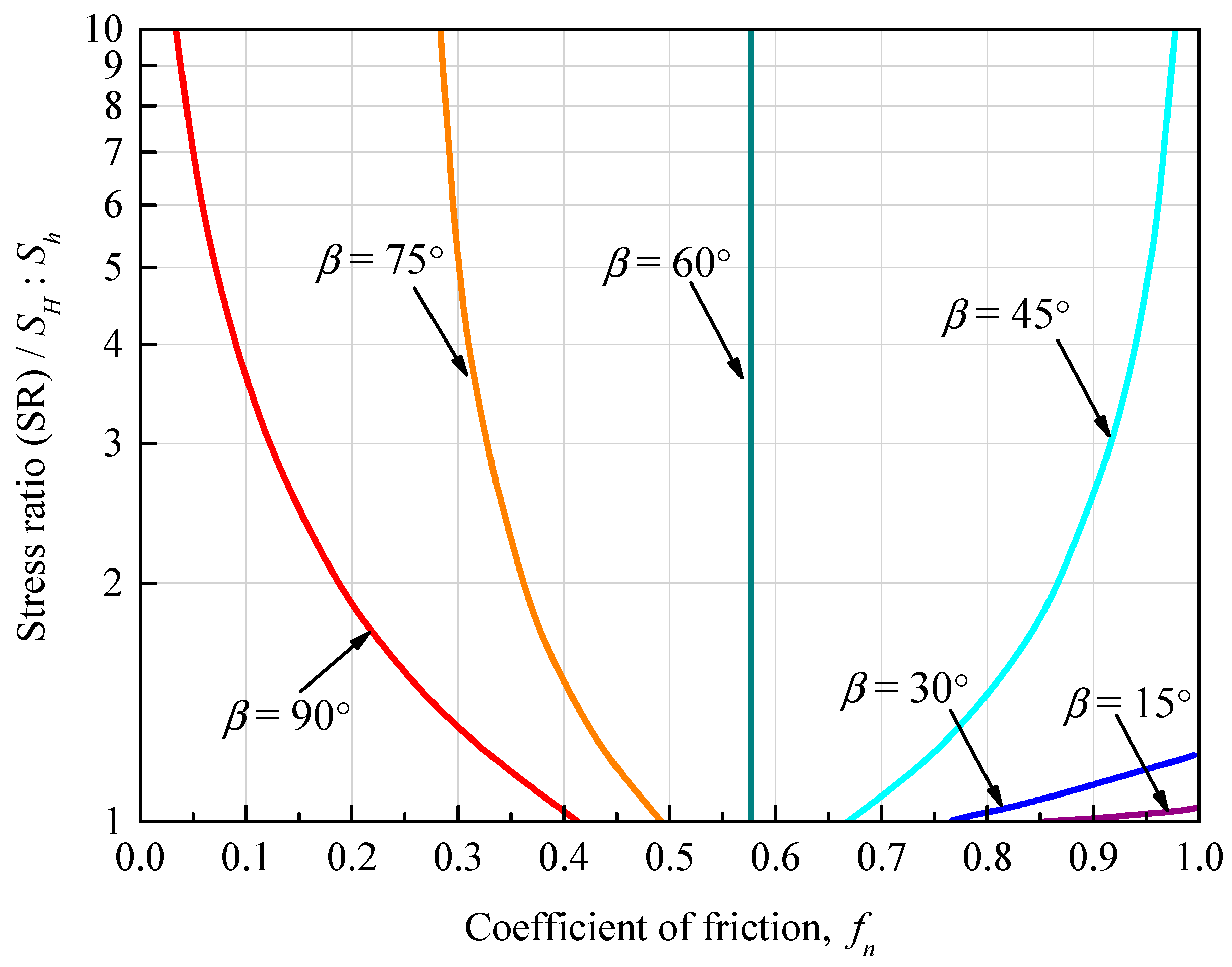
Figure 3.
(a) Coupled hydro-mechanical model; (b) Pore pressure build up; (c) Domain and flow channel; and (d) Hydraulic aperture.
Figure 3.
(a) Coupled hydro-mechanical model; (b) Pore pressure build up; (c) Domain and flow channel; and (d) Hydraulic aperture.
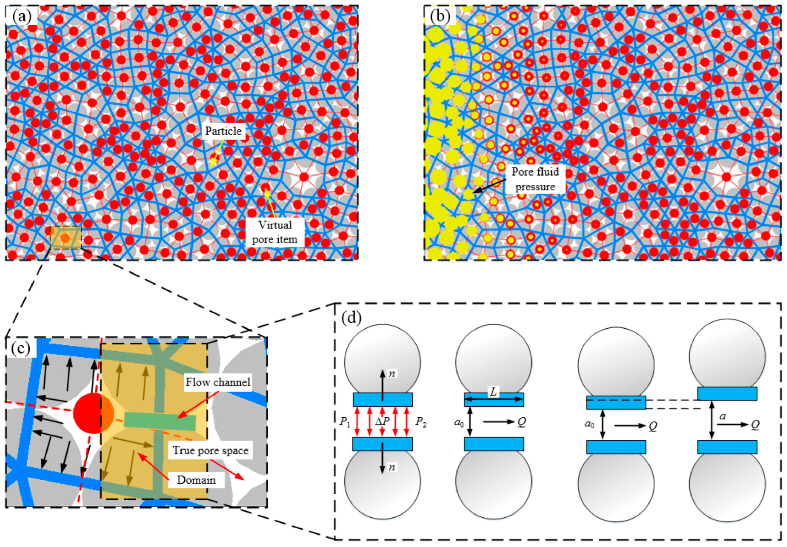
Figure 4.
Bond breakage and fluid pressure balancing according to Equation (4) in the two domains. (a) Fluid pressure before a crack initiation; (b) Fluid pressure after a crack initiation.
Figure 4.
Bond breakage and fluid pressure balancing according to Equation (4) in the two domains. (a) Fluid pressure before a crack initiation; (b) Fluid pressure after a crack initiation.

Figure 5.
Definition of the same seismic event in terms of space, in which Cracks 1, 2, and 3 belong to the same seismic event.
Figure 5.
Definition of the same seismic event in terms of space, in which Cracks 1, 2, and 3 belong to the same seismic event.

Figure 6.
Definition of the same seismic event in terms of time; the occurrence order of cracks is Crack 1, 5, 2, 3, and 4, where Cracks 1, 2, and 3 belong to the same seismic event.
Figure 6.
Definition of the same seismic event in terms of time; the occurrence order of cracks is Crack 1, 5, 2, 3, and 4, where Cracks 1, 2, and 3 belong to the same seismic event.
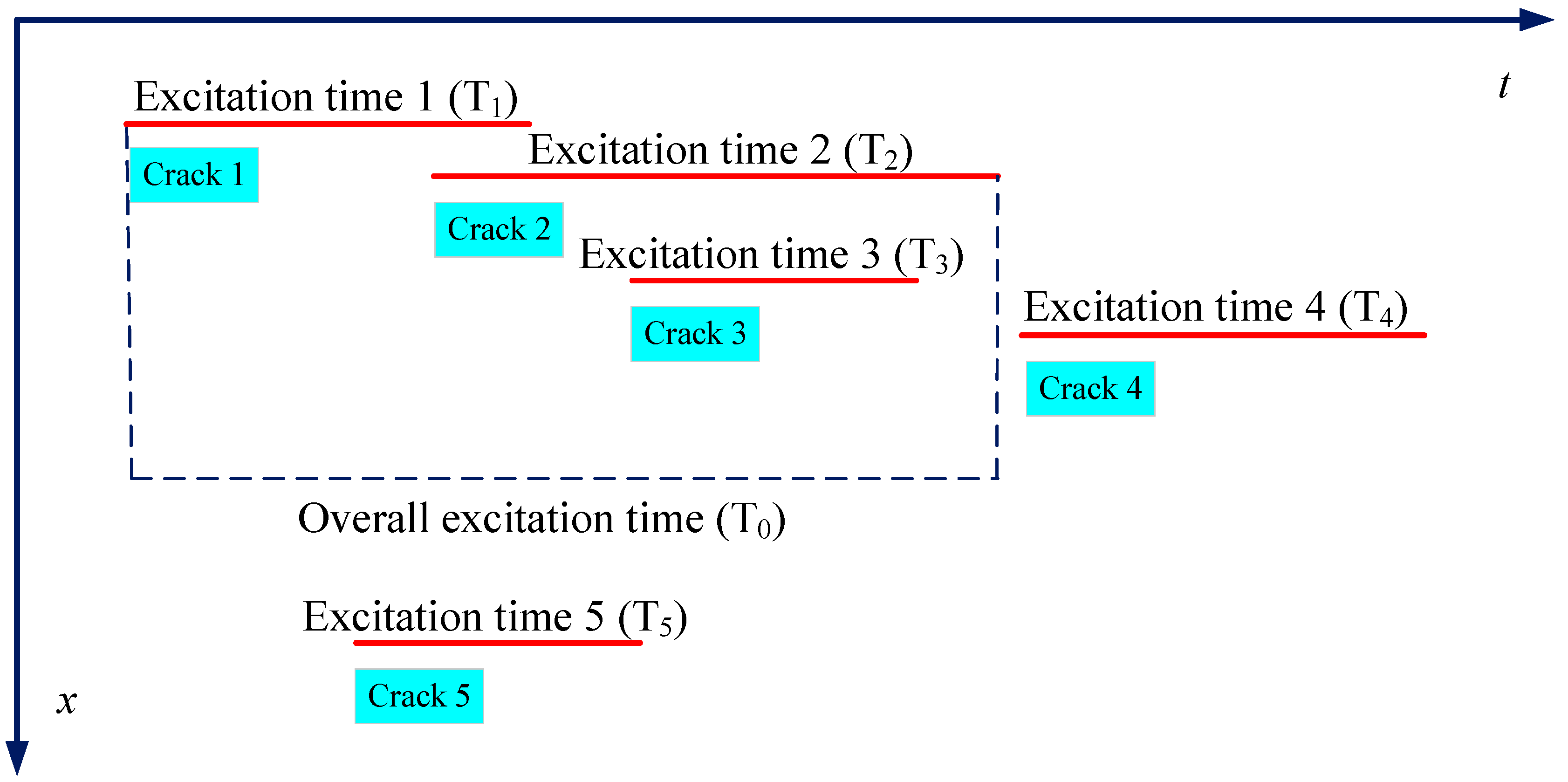
Figure 7.
(a) Distribution of shale gas enrichment basins and (b) the Marcellus shale play in the USA [42].
Figure 7.
(a) Distribution of shale gas enrichment basins and (b) the Marcellus shale play in the USA [42].
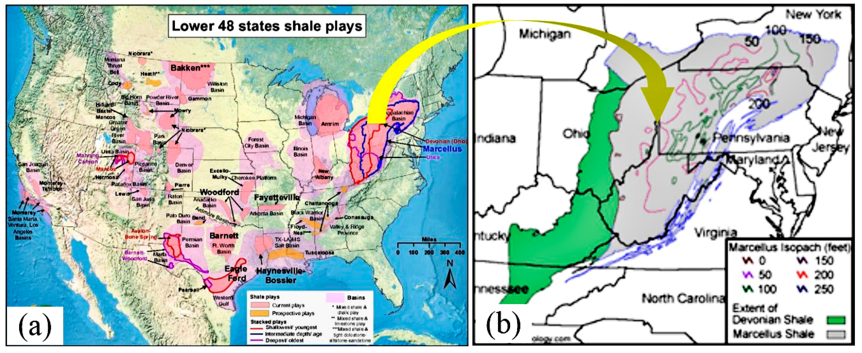
Figure 8.
Geometry reservoir model for hydraulic fracturing simulation: (a) sketch map of simulation model; (b) measurement region setup.
Figure 8.
Geometry reservoir model for hydraulic fracturing simulation: (a) sketch map of simulation model; (b) measurement region setup.
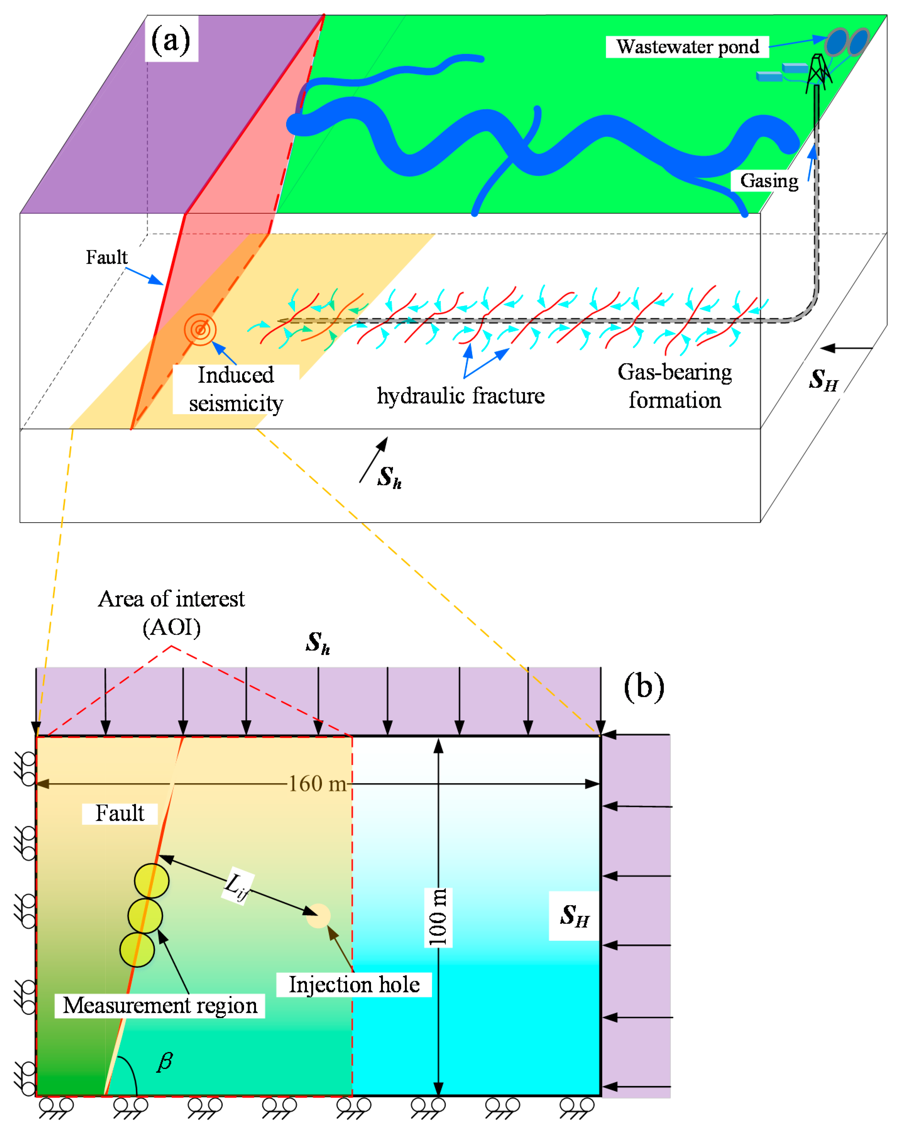
Figure 9.
Comparison results between numerical simulations and analytical solutions [20]: (a) β = 90°; (b) β = 75°; (c) β = 60°; (d) β = 45°; (e) β = 30°; and (f) β = 15°.
Figure 9.
Comparison results between numerical simulations and analytical solutions [20]: (a) β = 90°; (b) β = 75°; (c) β = 60°; (d) β = 45°; (e) β = 30°; and (f) β = 15°.
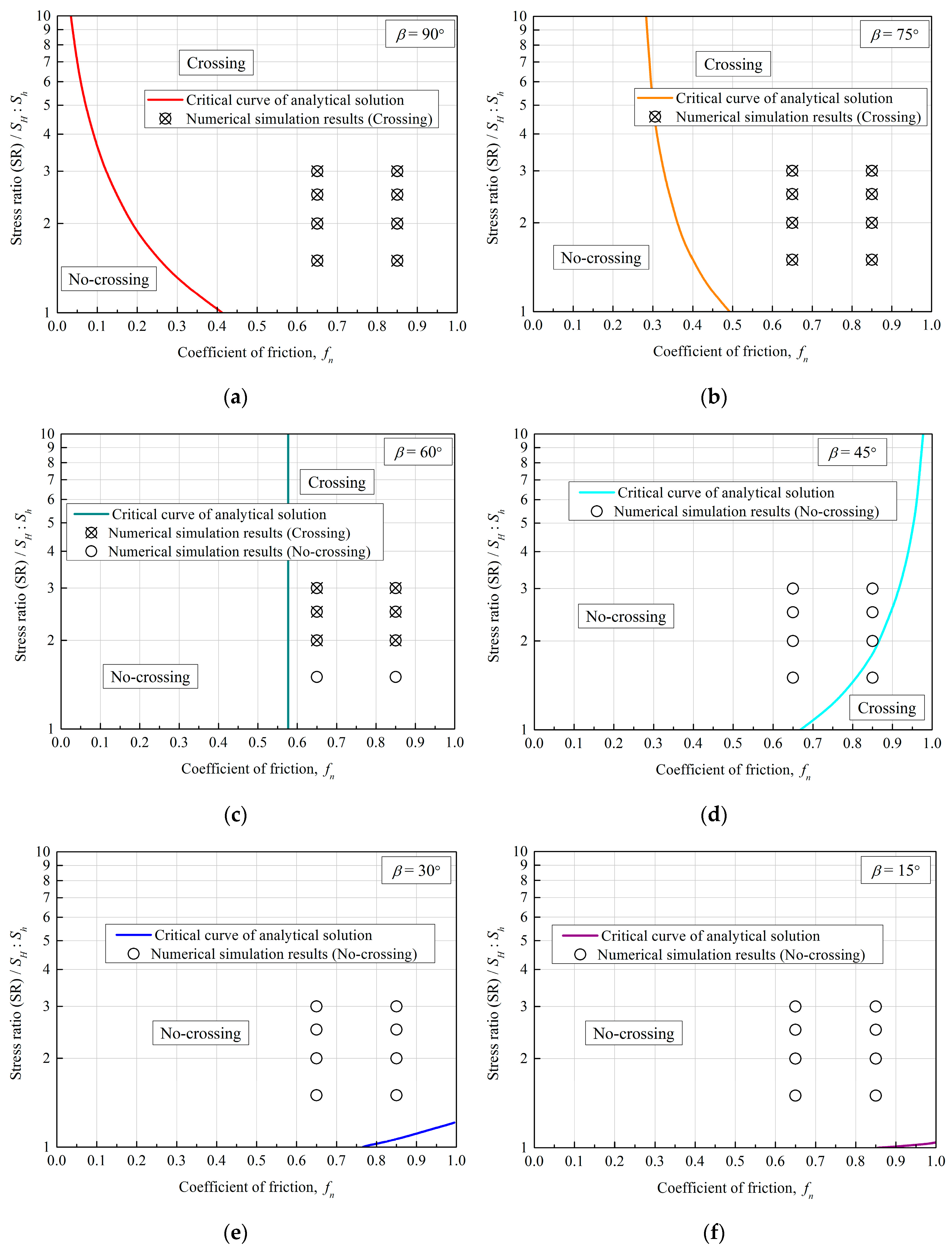
Figure 10.
Hydraulic fracture (HF) and fault interaction behavior for the numerical simulations performed under the friction coefficient of the fault: (a) fn = 0.27; and (b) fn = 0.58.
Figure 10.
Hydraulic fracture (HF) and fault interaction behavior for the numerical simulations performed under the friction coefficient of the fault: (a) fn = 0.27; and (b) fn = 0.58.

Figure 11.
A representative curve for fault slip displacement.

Figure 12.
Change of displacement of fault slip when the distance between the injection hole and the fault ranged from 10 to 60 m.
Figure 12.
Change of displacement of fault slip when the distance between the injection hole and the fault ranged from 10 to 60 m.

Figure 13.
Change of normalized range of fault activation when the distance between the injection hole and the fault ranged from 10 to 60 m.
Figure 13.
Change of normalized range of fault activation when the distance between the injection hole and the fault ranged from 10 to 60 m.
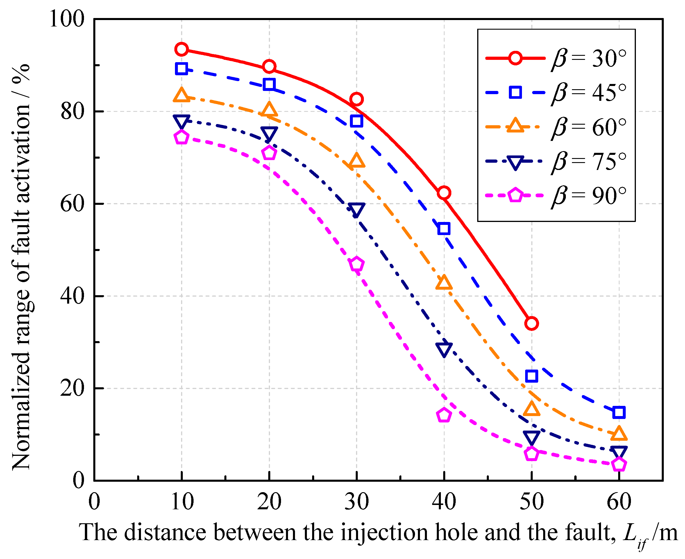
Figure 14.
Simulated injection-induced seismic events with variation in the distance between the injection hole and the fault: (a) Lif = 10 m; (b) Lif = 20 m; (c) Lif = 30 m; (d) Lif = 40 m; (e) Lif = 50 m; and (f) Lif = 60 m.
Figure 14.
Simulated injection-induced seismic events with variation in the distance between the injection hole and the fault: (a) Lif = 10 m; (b) Lif = 20 m; (c) Lif = 30 m; (d) Lif = 40 m; (e) Lif = 50 m; and (f) Lif = 60 m.

Figure 15.
Distribution of injection pressure with variation of the distance between the injection hole and the fault: (a) Lif = 10 m; (b) Lif = 20 m; (c) Lif = 30 m; (d) Lif = 40 m; (e) Lif = 50 m; and (f) Lif = 60 m.
Figure 15.
Distribution of injection pressure with variation of the distance between the injection hole and the fault: (a) Lif = 10 m; (b) Lif = 20 m; (c) Lif = 30 m; (d) Lif = 40 m; (e) Lif = 50 m; and (f) Lif = 60 m.
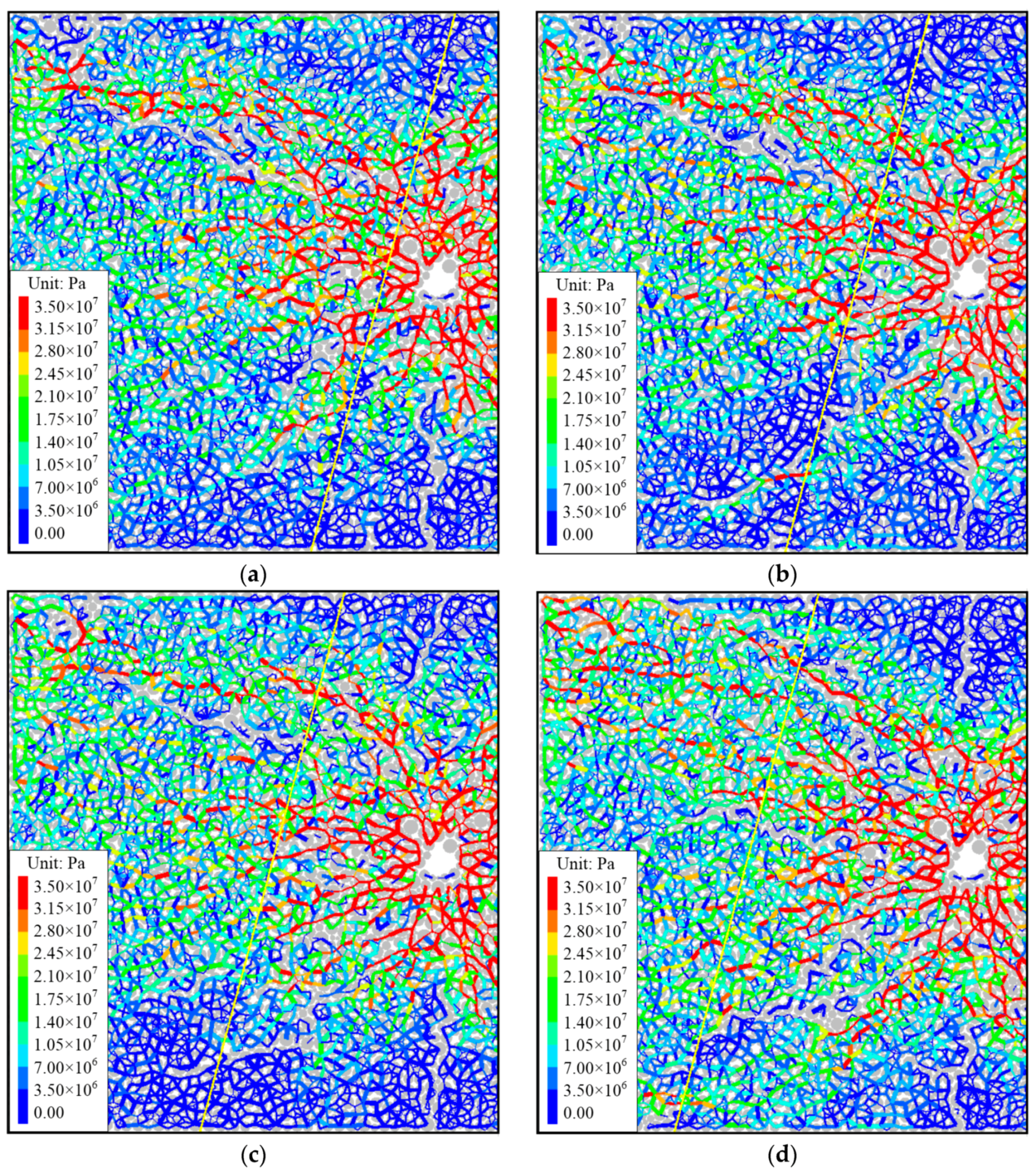
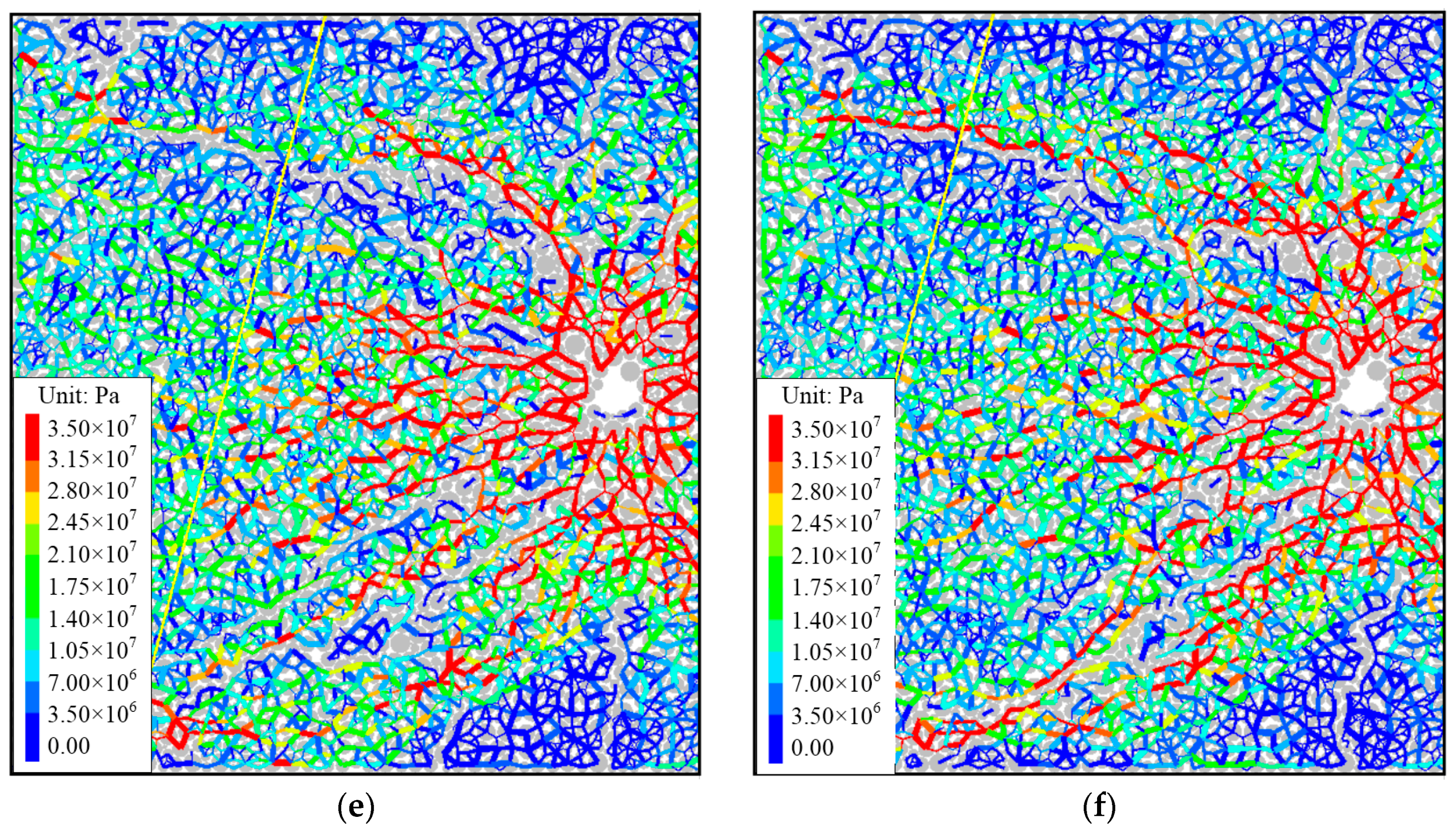
Figure 16.
Relationship between the magnitude of seismic events and the logarithmic seismic events when the distance between the injection hole and the fault ranged from 10–60 m.
Figure 16.
Relationship between the magnitude of seismic events and the logarithmic seismic events when the distance between the injection hole and the fault ranged from 10–60 m.
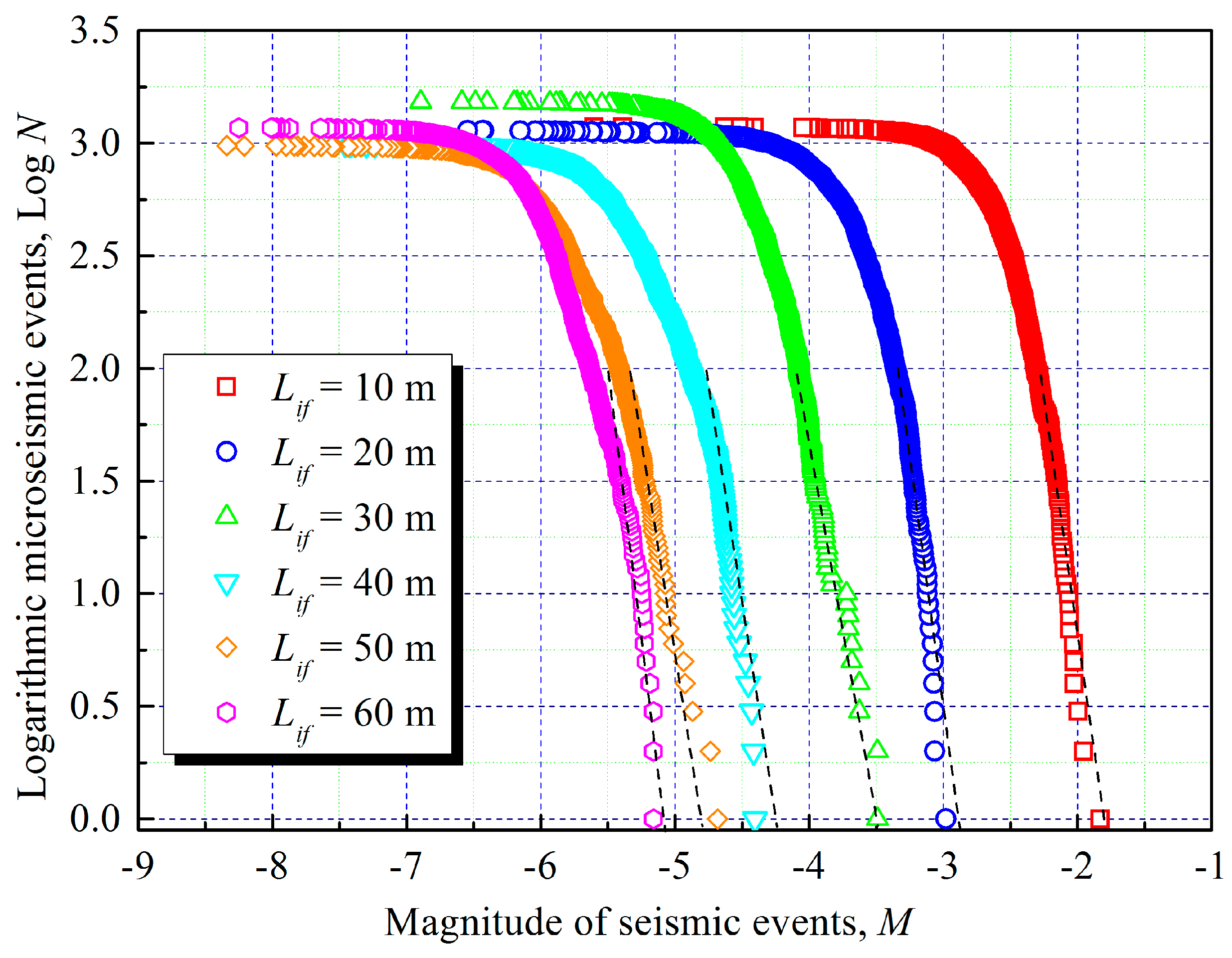
Figure 17.
Variations in borehole pressure and magnitude of seismic events when the distance between the injection hole and the fault ranged from 10–60 m: (a) Lif = 10 m; (b) Lif = 20 m; (c) Lif = 30 m; (d) Lif = 40 m; (e) Lif = 50 m; and (f) Lif = 60 m.
Figure 17.
Variations in borehole pressure and magnitude of seismic events when the distance between the injection hole and the fault ranged from 10–60 m: (a) Lif = 10 m; (b) Lif = 20 m; (c) Lif = 30 m; (d) Lif = 40 m; (e) Lif = 50 m; and (f) Lif = 60 m.


Figure 18.
Relationship between the magnitude of seismic events and the frequency of seismic events with different injection sites: (a) Lif = 10 m; (b) Lif = 20 m; (c) Lif = 30 m; (d) Lif = 40 m; (e) Lif = 50 m; and (f) Lif = 60 m.
Figure 18.
Relationship between the magnitude of seismic events and the frequency of seismic events with different injection sites: (a) Lif = 10 m; (b) Lif = 20 m; (c) Lif = 30 m; (d) Lif = 40 m; (e) Lif = 50 m; and (f) Lif = 60 m.
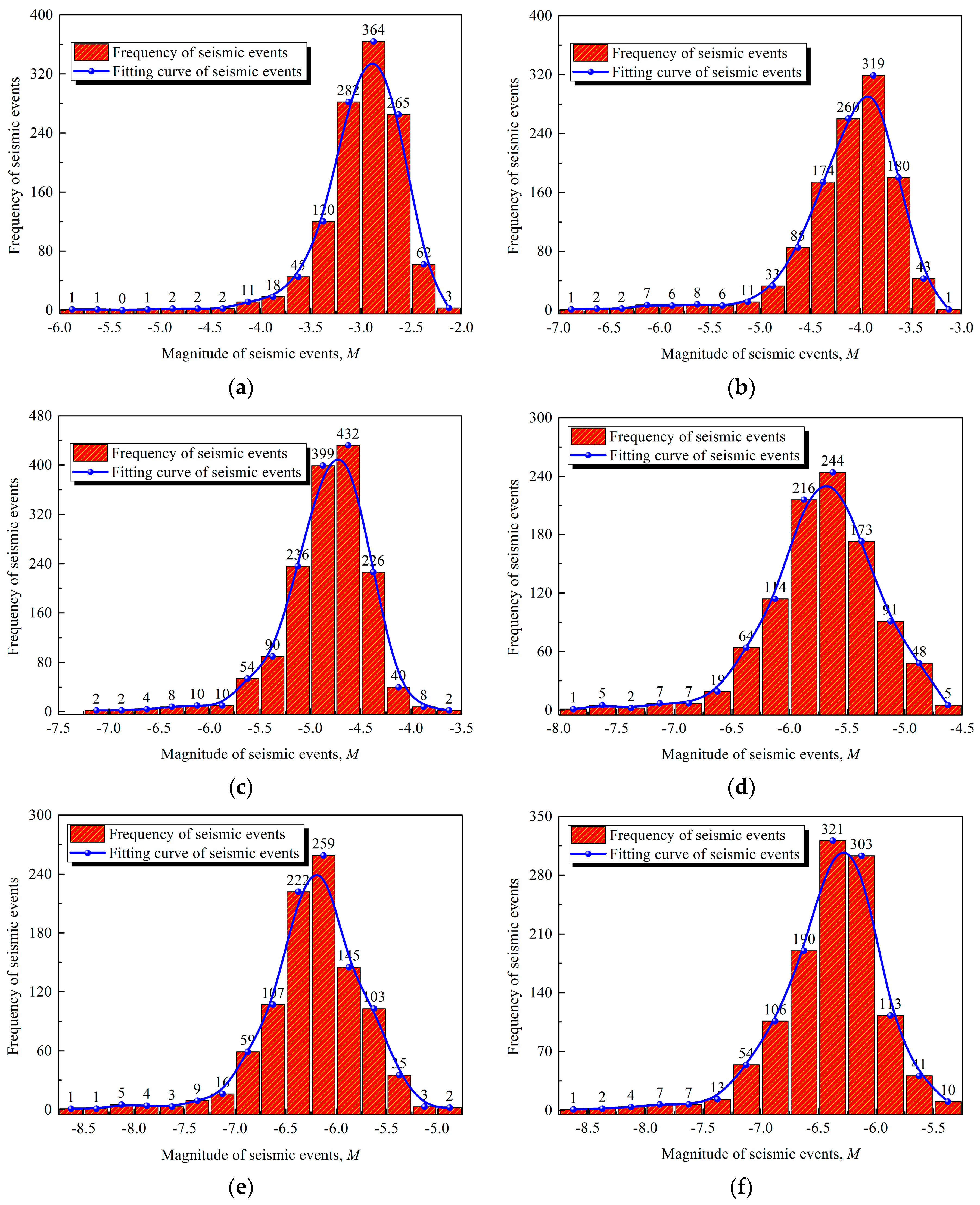
Figure 19.
Relationship between the frequency of seismic events and the number of cracks of every seismic event containing different injection sites: (a) Lif = 10 m; (b) Lif = 20 m; (c) Lif = 30 m; (d) Lif = 40 m; (e) Lif = 50 m; and (f) Lif = 60 m.
Figure 19.
Relationship between the frequency of seismic events and the number of cracks of every seismic event containing different injection sites: (a) Lif = 10 m; (b) Lif = 20 m; (c) Lif = 30 m; (d) Lif = 40 m; (e) Lif = 50 m; and (f) Lif = 60 m.


Table 1.
Micro-properties used for the simulated model after calibration. PB: parallel bond; SJ: smooth joint.
Table 1.
Micro-properties used for the simulated model after calibration. PB: parallel bond; SJ: smooth joint.
| Parameters | Unit | Values |
|---|---|---|
| Rock Matrix | ||
| Particle density | kg/m3 | 2700 |
| Particle friction coefficient | - | 0.10 |
| Young’s modulus of the particle | GPa | 15.2 |
| Young’s modulus of the parallel bond | GPa | 15.2 |
| Normal stiffness of the parallel bond (mean) | MPa | 100.6 |
| Normal stiffness of the parallel bond (std deviation) | MPa | 25 |
| Shear stiffness of the parallel bond (mean) | MPa | 131.5 |
| Shear stiffness of the parallel bond (std deviation) | MPa | 30 |
| Fault Properties | ||
| Normal stiffness | GPa/m | 60 |
| Shear stiffness | GPa/m | 60 |
| Tensile strength | MPa | 0 |
| Cohesion | MPa | 0 |
| Friction angle | ° | 29.5 |
| Dilation angle | ° | 0 |
| Fluid Properties and Operational Parameters | ||
| Injection rate | m3·s−1 | 2.0 × 10⁻⁶ |
| Fluid bulk modulus | GPa | 2.2 |
| Fluid dynamic viscosity | Pa·s | 1.1 × 10⁻⁴ |
| Initial hydraulic aperture | m | 3.2 × 10⁻⁵ (PB and SJ) |
| Infinite hydraulic aperture | m | 3.2 × 10⁻⁶ (PB and SJ) |
Table 2.
Fault properties assigned for the proposed models.
| Parameters | Unit | Values |
|---|---|---|
| Normal stiffness | GPa/m | 45 |
| Shear stiffness | GPa/m | 45 |
| Tensile strength | MPa | 6.2 |
| Cohesion | MPa | 4.8 |
| Friction angle | ° | 23.5 |
| Dilation angle | ° | 0 |
Table 3.
Duration time and fault slip displacement at four stages when the distance between the injection hole and the fault ranged from 10 to 60 m.
Table 3.
Duration time and fault slip displacement at four stages when the distance between the injection hole and the fault ranged from 10 to 60 m.
| The Distance between the Injection Hole and the Fault (m) | 10 | 20 | 30 | 40 | 50 | 60 | |
|---|---|---|---|---|---|---|---|
| Stage I | Duration (min) | 4.70 | 9.34 | 14.28 | 20.16 | 24.32 | 29.44 |
| Displacement (mm) | 0 | 0 | 0 | 0 | 0 | 0 | |
| Stage II | Duration (min) | 4.24 | 7.9 | 7.02 | 6.96 | 6.06 | 5.90 |
| Displacement (mm) | 104.11 | 81.96 | 63.09 | 42.41 | 16.07 | 15.13 | |
| Stage III | Duration (min) | 30.48 | 22.54 | 19.98 | 14.96 | 12.6 | 9.19 |
| Displacement (mm) | 33.29 | 39.83 | 29.28 | 22.98 | 22.97 | 11.28 | |
| Stage IV | Duration (min) | 20.58 | 20.22 | 18.72 | 17.92 | 17.02 | 15.47 |
| Displacement (mm) | 5.87 | 3.77 | 3.57 | 2.54 | 2.95 | 2.57 | |
| Accumulative displacement (mm) | 143.27 | 125.56 | 95.94 | 67.93 | 41.99 | 28.98 | |
Table 4.
Fitting a- and b-values of the accumulated seismic events when the distance between the injection hole and the fault ranged from 10–60 m.
Table 4.
Fitting a- and b-values of the accumulated seismic events when the distance between the injection hole and the fault ranged from 10–60 m.
| The Distance between the Injection Hole and the Fault (m) | a-Value | b-Value |
|---|---|---|
| 10 | −11.79 | 2.52 |
| 20 | −8.928 | 2.96 |
| 30 | −20.23 | 3.65 |
| 40 | −9.07 | 4.85 |
| 50 | −16.26 | 6.01 |
| 60 | −21.48 | 7.20 |
© 2017 by the authors. Licensee MDPI, Basel, Switzerland. This article is an open access article distributed under the terms and conditions of the Creative Commons Attribution (CC BY) license (http://creativecommons.org/licenses/by/4.0/).
Share and Cite
MDPI and ACS Style
Chong, Z.; Li, X.; Chen, X. Effect of Injection Site on Fault Activation and Seismicity during Hydraulic Fracturing. Energies 2017, 10, 1619. https://doi.org/10.3390/en10101619
AMA Style
Chong Z, Li X, Chen X. Effect of Injection Site on Fault Activation and Seismicity during Hydraulic Fracturing. Energies. 2017; 10(10):1619. https://doi.org/10.3390/en10101619
Chicago/Turabian StyleChong, Zhaohui, Xuehua Li, and Xiangyu Chen. 2017. "Effect of Injection Site on Fault Activation and Seismicity during Hydraulic Fracturing" Energies 10, no. 10: 1619. https://doi.org/10.3390/en10101619
Note that from the first issue of 2016, this journal uses article numbers instead of page numbers. See further details here.