Sensitivity Analysis of Time Length of Photovoltaic Output Power to Capacity Configuration of Energy Storage Systems

Abstract

Time interval and time length are two important indexes when analyzing the active output data of photovoltaic (PV) power stations. When the time interval is constant, the length of time is too small, and the included information is less, resulting in a lack and distortion of information; it the length of time is too large, the included information is redundant and complicated, resulting in unnecessary increases of storage capacity and calculation. Therefore, it is important to determine the appropriate length of data for the analysis of PV output data. In this paper, firstly, the output data of a PV power station is analyzed statistically, and the preliminary conclusions for time length selection are obtained by autocorrelation analysis. Based on the weather characteristics, clustering analysis methods and statistical principles are used to analyze the data and optimal sample capacity estimation, respectively, for different types of photovoltaic output data and determine the required data time length at the time of analyzing the PV power plant output data, the relationship between energy storage capacity demand and data length is investigated, the rationality of the length of the selected time is verified. Meanwhile, the energy storage system capacity configuration based on the optimal data time length is given. The results show that the requirement of data volume of energy storage system capacity configuration can be met when the time length of the PV output data is 23 days.

1. Introduction

Photovoltaic (PV) power generation as a clean and rich renewable energy source has attracted the attention of scholars at home and abroad [1,2,3]. At present, the research on PV power generation is becoming more and more mature, mainly in the areas of power prediction [4,5], optimal control [6,7], and energy storage system capacity optimization [8,9,10,11,12] for PV power stations. The essence of the above questions is the excavation and analysis of the information contained in the PV output data. A large number of data is stored in PV power plant databases. When analyzing PV output data, we need to consider the degree of density of the data collection and the amount collected, that is, the data interval and time length. Data volume is equal to the ratio of time length to time interval. In the joint application occasion of energy storage and renewable energy power generation and under the premise of not harming to the characteristics of the system, choosing the sampling time length scientifically and then recording the power output trajectory of intermittent power supply, is the foundation to grasp the system characteristics accurately and optimized the utilization. In this paper, we analyze in depth the power output data of a PV power plant, quantify the length of time and analyze and verify the result in the storage power station. The method can provide the most effective collection of time data under the condition of maximum economic cost savings, which has engineering practicality.

It can be seen that the overall length of data decreases and the overall data volume reduces linearly when the acquisition time interval is constant, but this easily leads to a shortage of the overall sample, the uncertainty increases, and the information is incomplete. When the overall data length increases, the amount of data rises, and the completeness of the sample uncertainty is enhanced, but this will produce redundancy, resulting in repetitive research and calculation. At present, studies on the overall length of time data have achieved some advances at home and abroad.

In [13], through the analysis of the sample information entropy change trend of the PV output power, a sampling span calibration method for the PV power output based on information entropy theory is proposed based on space characteristics. The simulation results show that the sampling span takes 33 days, which can satisfy the need for accuracy of the required energy storage system data to realize the smooth control of the PV output power. In [14], information entropy is used to measure the smoothness of the data and a selection method for the training sample length based on information entropy is proposed. Appropriate training samples were selected, and the data length was reduced, saving learning time and meanwhile the accuracy of the forecast results is improved. In [15], the length of the sample used in modeling the parametric model is discussed, analyzing the differences between different sample numbers used in the modeling. It is considered that the number of model samples has no significant effect on the estimation of model parameters, especially, when the sample length is short, which will have a great influence and must be carefully considered when modeling. In [16], a method for estimating the required sample length under the given analytical precision conditions by using the mean square value of variance coefficient curve equation is presented. Using this method, a mathematical model of the mean square deviation coefficient can be established with a finite but sufficient amount of test data to derive the necessary sample length with the required accuracy. In [17], a decision tree analysis is carried out by considering the function form of the model based on the Fisher information approximation method and the three competing models. In [18], the Monte Carlo process is used to propose a sample size and size spatial correlation function and reduce the data of spatial statistics by describing the matrix and elliptical contours and using the maximum likelihood method. In [19], the effects of different sampling strategies and sample size on the results of the study are investigated during the analysis of the relationship between trees and topography. In [20], a model predictive control scheme is assessed and its performance studied and compared to a thermostat with the aim of minimizing the cooling energy consumption through the minimization of the energy cost while satisfying the adequate temperature range for the human comfort. In [21], a model-based predictive control approach is proposed for home cooling and heating systems. Its effectiveness is compared to conventional thermostat control by providing simulations covering 24 h in a household. In [22], introduce a new consumption reduction method in some residential loads via the implementation of model predictive control. In [23], the impact of model predictive control on energy savings of residential households is determined. The value and impact of power generated by local power sources, such as roof-top-solar, will be determined during off-peak, mid-peak and on-peak, providing simulations during 24 h in a house. In [24], the research theme is focused on the relation between model predictive control weighting adjustment and the minimization of energy consumption. In general, at present the time length of the data samples used in different researches is different, and there is no definite theoretical guidance and method to base the selection. The means that analyses of the influence of the change of the time length of the collection sample on the system modeling are also limited to make repetitive horizontal contrasts between the time series of the different sample time lengths, without mining the characteristics of the time series, which lack qualitative or quantitative analysis. In this paper, based on the characteristics of the PV power time series, a quantitative analyzed standard of the sampling time length on the energy storage capacity sensitivity is given.

Since the study of the total length of data for renewable energy output data is not mature, this paper analyzes the capacity optimization problem of energy storage system arranged in a PV power plant as an example. Many of the studies select the total data length as one day [9] or one year [10,11,12] and inevitably must reconsider and calculate the data of many similar characteristic days. In this paper, we use the autocorrelation analysis to initially determine the suitable time length of the sample to meet the requirements of the data volume of the PV power plant. Then we use cluster analysis to analyze the fluctuations of the PV power data under five typical weather conditions. Finally, by using the most suitable sample estimation method under typical weather conditions we determine an optimal sampling time length that satisfies the data volume analysis requirements. This paper aims at PV output data of 45 s [25] and 60 s [13] interval to perform the analysis and determine the mathematical statistics. Given a method for determining the time length, then then analyze and verify it through investigating the relationship between the length of PV and the energy storage capacity of a PV power plant.

2. Analysis of the Output Characteristics of Photovoltaic Power Stations

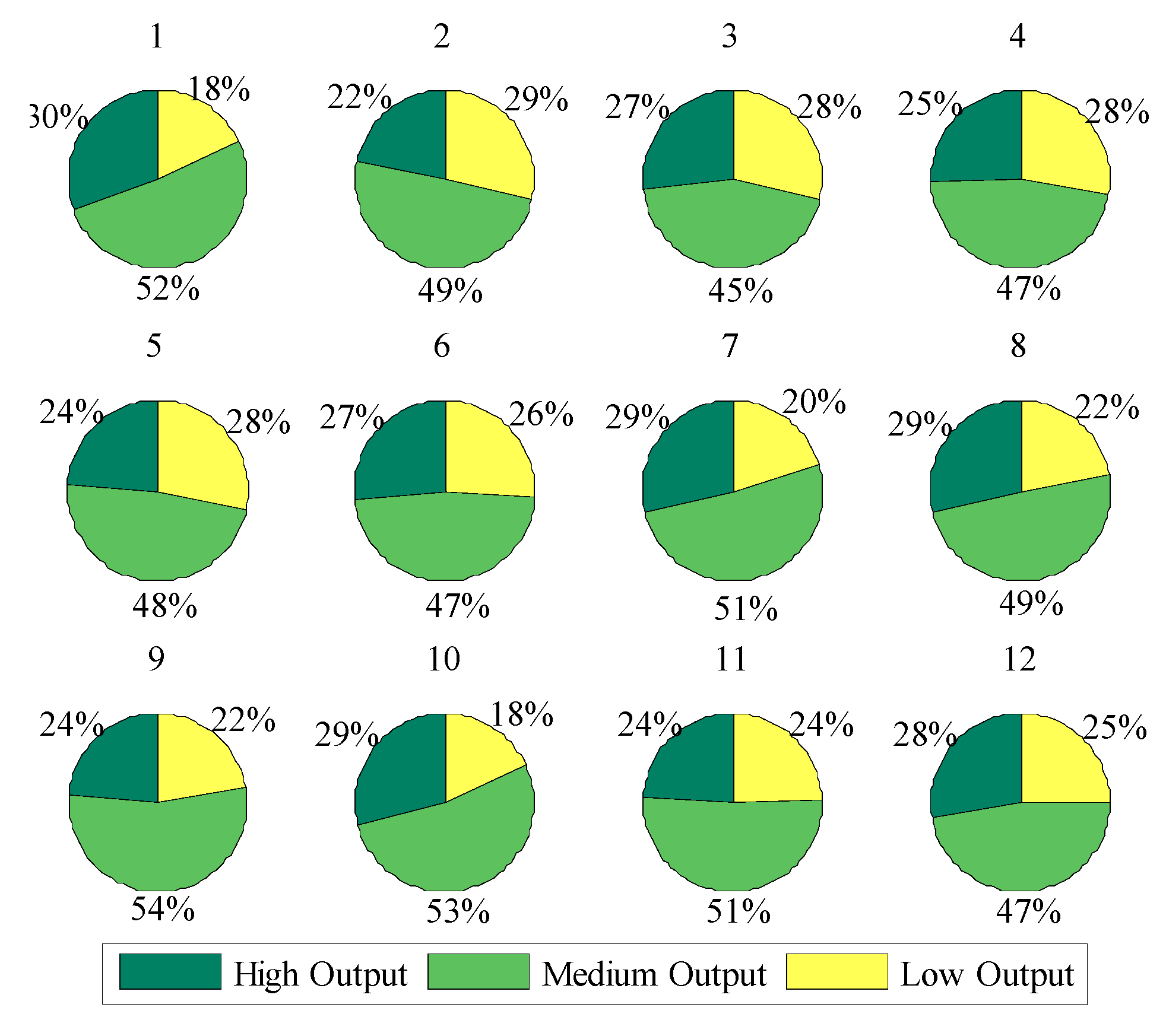
2.1. Output Power Level Statistics

The output of PV power plants depends on natural conditions such as the light intensity and ambient temperature. It is helpful for the dispatching department to arrange the power generation plan reasonably to master the distribution regulation of PV power generation in time and place. Therefore, the datamining analysis of the PV power plant operation data should first focus on the output power level of the plant. Taking some PV power plants with installed capacities of 40, 25 and 14 MW as examples (the data comes from the Zhangjiakou wind-photovoltaic-storage project of the State Grid Corporation in Hebei Province, China), we use the quantitative analysis method to analyze the time and place distribution of the PV power plant output data during 1 year. The output level of the PV plant is defined as the percentage of installed capacity, as shown in

Table 1. The definition of the output level of the PV plant.

Output Level	Definition
High output	The output level is higher than 60% of the installed capacity
Medium output	The output level is between 30% and 60% of the installed capacity
Low output	The output level is lower than 30% of the installed capacity

.

According to this definition, we do a statistical analysis of the percentage of the high, medium and low output operating times and find the proportion of them accounting for total output time in that month of the PV power station. Then we calculate the output level distribution figure of each month of the PV power station, which is shown in Figure 1.

It can be seen from the figure that the proportion of the three high, medium and low output levels in each month are approximately the same, but is not exactly, and the proportion of medium output accounting for the proportion of each month is about half, while the high output and low output account for a low proportion. This is consistent with the statistical outcome of the weather and illumination conditions in this area. This completes the macroscopic understanding of the power output level of the PV power station.

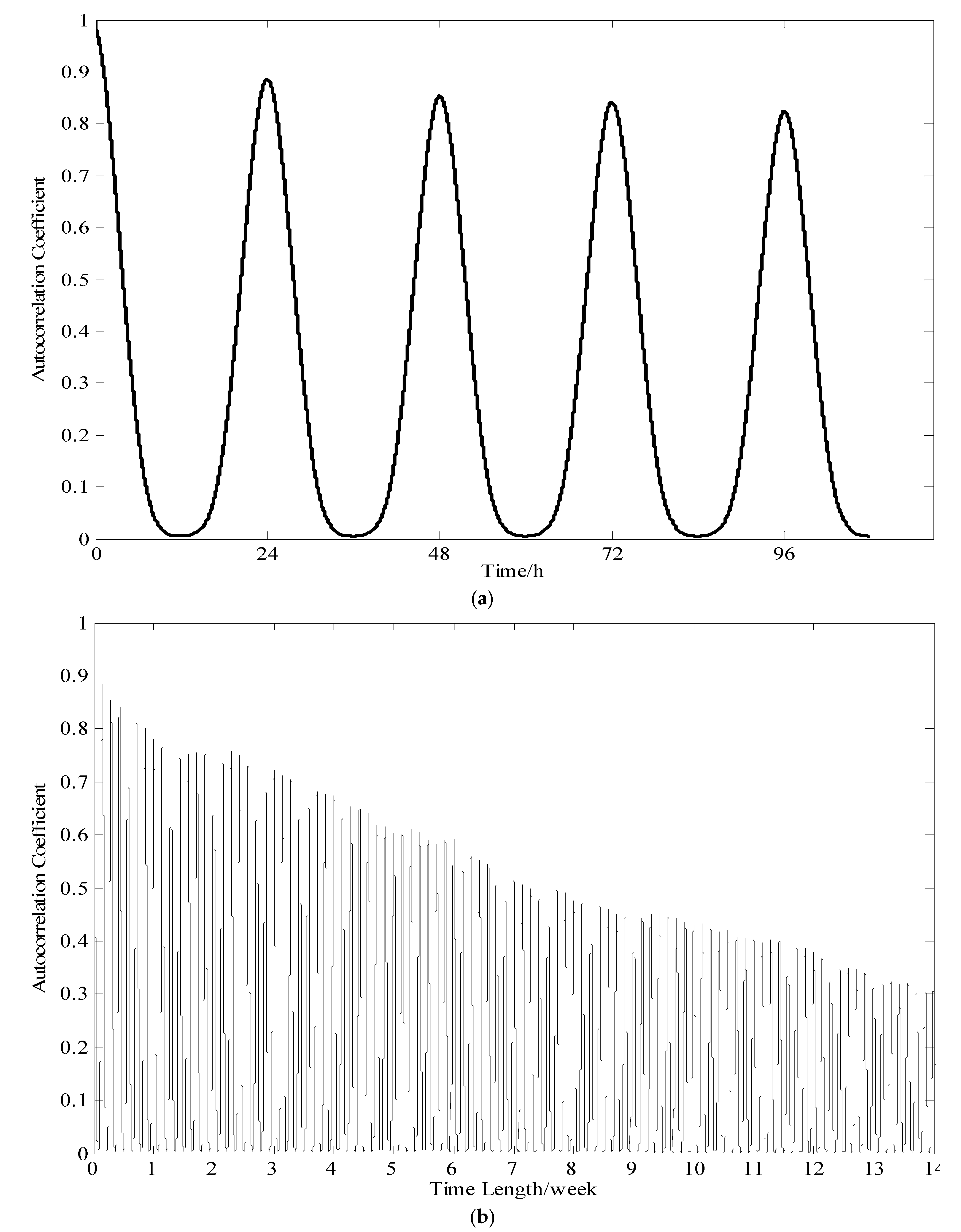
2.2. Output Data Autocorrelation Analysis

The time series (or dynamic numerical sequence) refers to a numerical sequence which arranges values of the same statistical indicators in accordance with the time order. Analyzing the time series can predict the future data based on historical data and help recognize the overall characteristics of this numerical sequence. The PV output data is regarded as a random time series. When analyzing the random time series, it is necessary to evaluate the correlation between the data of any moment and the historical data in order to discover the implicit laws and periodicity in the sequence. These characteristics can be obtained by analyzing the autocorrelation characteristics of the sequence.

The basis of autocorrelation analysis is the correlation coefficient in statistics, which is calculated as follows:

$${\rho }_{xy}=\frac{\mathrm{cov}(x_t,y_t)}{\sqrt{\mathrm{var}(x)\cdot \mathrm{var}(y)}}$$

(1)

Here, cov(•) expresses covariance and var(•) expresses variance. The correlation coefficient describes the consistency of the numerical variation trends among different sequences. The greater the absolute value of the correlation coefficient is, the stronger the change correlation between the sequences becomes.

When a time sequence is moved under time displacements to get another sequence, the correlation coefficient between the two sequences is also called the autocorrelation coefficient. The autocorrelation coefficient describes the consistency of change between the current data and the data before the moment Δt, and Δt is the time displacements. Do a correlation analysis of PV output data through calculating autocorrelation coefficients, as shown in Figure 2.

Figure 2a shows that with the change of length of time, the autocorrelation coefficient presents a decreasing and oscillating trend and the oscillation cycle is 24 h, which shows that if we use 24 h as the PV output period, the output will have an obvious and regular changing trend, so taking one-day data as the basic unit to determine the time length of data is reasonable. From the view of Figure 2b, with the time length increasing, the oscillation amplitude of the autocorrelation coefficient is decreasing and the oscillation center is approaching the 0 point. After more than 2400 h (100 days), the autocorrelation coefficient maximum value of PV sequence drops below 0.3 [26,27,28], Thus, we can think that correlation between the PV output at any time and PV output historical data changes before 100 days is weak, and its influence is very small. Therefore, in the three PV power plant capacity scenarios, it is concluded that we should take 100 days as a time length sample to analyze the PV output data.

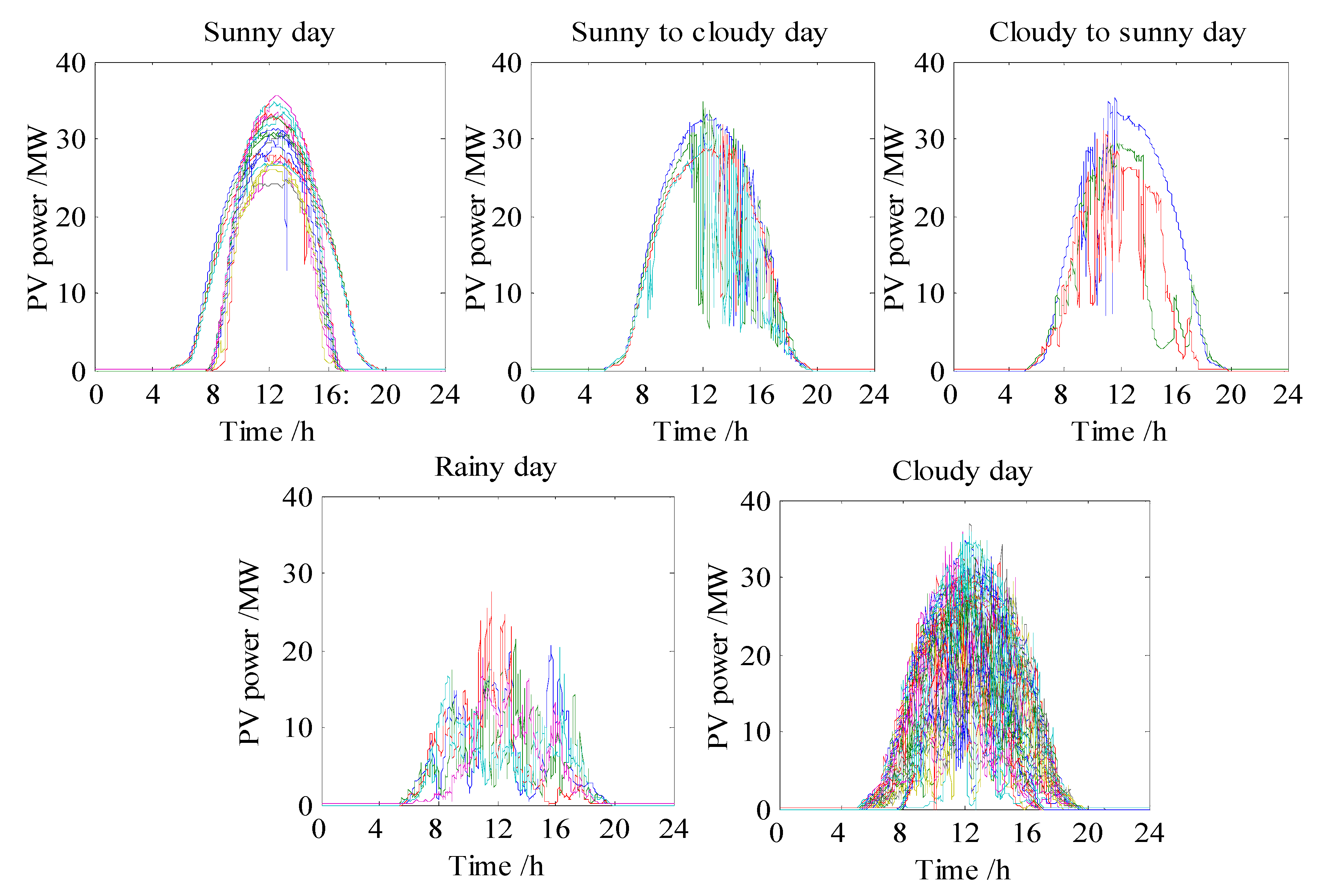
2.3. The Clustering Analysis of Similar Day of Operation Data of the PV Power Station

After comparing between the operation data output level of the PV power plant and the weather conditions, and further analyzing the data, we note that a high output level corresponds to sunny days, a low output level corresponds to rainy days, while the output level has three kinds of weather conditions: clear turning to cloudy, cloudy turning to clear and cloudy. The analysis of the output level of operation data of the PV power plant describes the generating capacity of the power station, but it cannot describe the fluctuating distribution conditions of the PV power plant output. The power generation and fluctuation of PV output are strongly related to the weather conditions and the analysis of operation data of a PV power station should take into account both the output level and the fluctuations. Typical output under different weather conditions is shown in Figure 3.

The PV output curve exhibits different shapes as the weather changes. The photovoltaic output of the same weather type contains similar information. Doing clustering analysis on the PV data with the same weather type, we select weather characteristic parameters like the solar radiation intensity, radiation time and air temperature, etc. as the clustering index of the PV output, that is, the daily feature vector:

$$X_i=[I_{hi},\stackrel{-}{I_{sh}},\stackrel{-}{I_{xi}},t_{hi},\stackrel{-}{t_{\mathrm{s}h}},\stackrel{-}{t_{xi}},T]$$

(2)

$I_{hi},\stackrel{-}{I_{sh}},\stackrel{-}{I_{xi}}$: maximum solar radiation intensity value, morning average value, afternoon average value of day i;

$t_{hi},\stackrel{-}{t_{\mathrm{s}h}},\stackrel{-}{t_{xi}}$: maximum temperature, morning average temperature, afternoon average temperature of day i;

$T$: The length of irradiation time of day i;

We use the Euclidean distance to describe the overall difference of various meteorological factors between any two days:

$$d_{ij=}\sqrt{{\displaystyle \sum _{k=1}^m{(x_{ik}-x_{jk})}^2}}$$

(3)

where k is the sequence number of the eigenvector; m is the number of eigenvectors.

According to the conclusion of Section 2.2, we select 100-days PV data as the time length to do the clustering analysis and divide the data into five categories: (1) sunny day, (2) clear turning to cloudy, (3) cloudy turning to clear, (4) rainy, (5) cloudy. The clustering effect is shown in Figure 4.

As can be seen from Figure 4, the output conditions of PV power plants and the weather conditions are strongly related. The output curve of the PV power plant of the same weather type is similar, that is, the fluctuation is similar to the output level. As sunny days may also have clouds blocking the sunlight, the output curve of category 1~category 3 in the sunny days will also have slight fluctuations. The differences between category 4 (rainy) and category 5 (cloudy) are that the solar irradiance is very small throughout a rainy day, so the output amplitude is very small; clouds is affected by the cloud movement, the sun is sometimes present, and sometimes disappears, so the amplitude of the output curve is greater than on rainy days and the fluctuation is more intense.

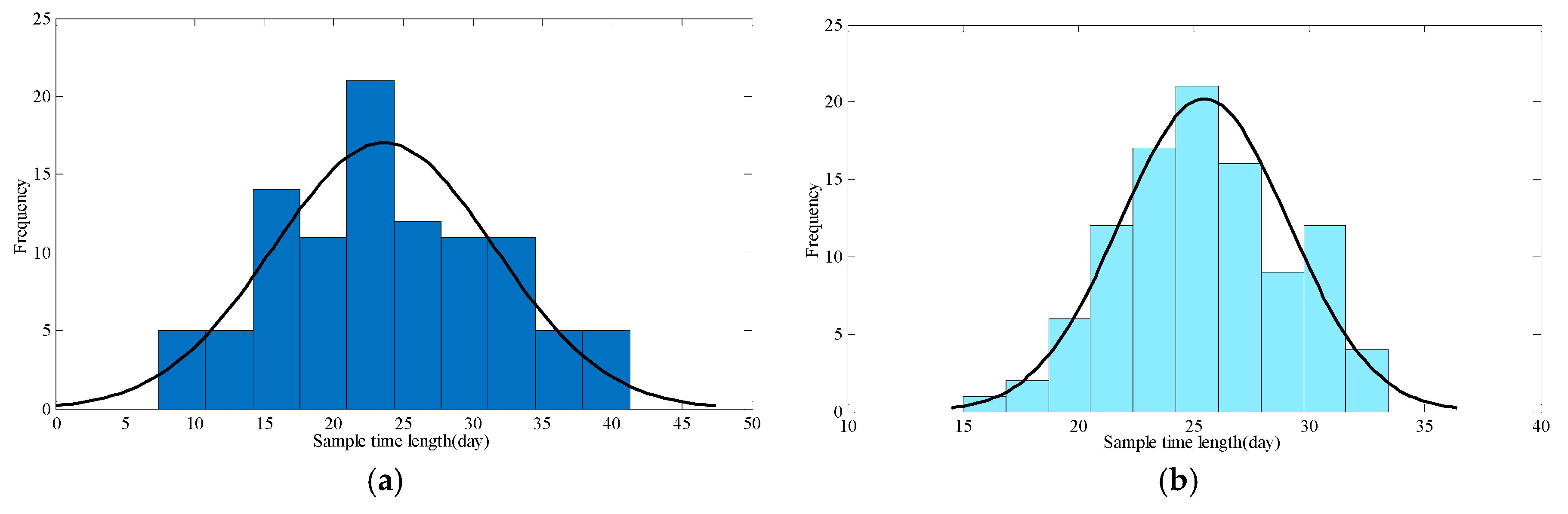
2.4. Based on the Optimal Sample Capacity Estimate to Determine the Length of Time

According to the conclusions obtained from the autocorrelation analysis, we take the one-day output curve of a PV power plant capacity as the sample unit and take one day as the step length to gradually increase the sample capacity. With the increase of the output day sample of the PV power plant, the different typical output characteristic days are becoming more and more complete, the amount of obtained information is more and more, the amount of data will also have a certain amount of redundancy. The key to the rational choice of data time length is not only to include the different output characteristics of the power station, but also to screen out the unnecessary redundant information, which requires research on the characteristics of the daily output data of the photovoltaic power plant.

The characteristics of daily output data of a PV power plant reflect the acute degree of fluctuation and size of power generation. In order to show the characteristics of any one-day output data of a PV power plant, we definite a daily output characterization coefficient B_i as:

$$B_i=\frac{N\cdot {\displaystyle \sum _{j=1}^N(P_{ij}-\frac{1}{N}{\displaystyle \sum _{j=1}^N{P}_{ij}})}{}^2}{{\displaystyle \sum _{j=1}^N{P}_{ij}}}$$

(4)

In the formula, P_ij is the power value of the jth sample point of Day i, and N is the number of every day total sampling points. The purpose of selecting the time length of the operation data of the PV plant is to find the most suitable sample capacity which can reflect the data characteristics, which in essence can abstract it as an optimal sample capacity estimation problem. According to the principle of probability and statistics, when doing an organization sample survey, the size of the sampling error directly affects the representative size of the sample index and the necessary sample unit number is an important factor to ensure the sampling error no more than the given range. Therefore, in the sampling design, it is necessary to determine the appropriate number of sample units, because the appropriate number of sample units is the basic premise to ensure the sample indicators are fully representative. In order to determine the time length of the operation data of the PV plant, we do an optimum sample size estimation on the daily output characterization coefficient under these five weather conditions: (1) sunny day, (2) clear turning to cloudy, (3) cloudy turning to clear, (4) rainy, (5) cloudy. The sum of the sample capacity estimation of all categories is the time length of the data.

The reason of doing optimal sample capacity estimation is that with regard to a large system state space, if we do consequence analysis on all the system state in order to get accurate results, it often lead to the calculation process into a “calculation of disaster”. Therefore, it is necessary to choose a random sample in the system state space and take the extracted sample on behalf of the overall level. The more the extracted samples are, the more comprehensive the feedback information is. However, in practical applications, the number of sampling points n cannot be too large, otherwise the calculation is too large, so we should allow errors ${\epsilon }_0$ based on the actual conditions and choose the value of n reasonably.

Set $(B_1,B_2,B_3,...,B_n)$ is a sample from B. $E(B)=u,D(B)={\sigma }^2$ By the central limit theorem, for real numbers $t_{\alpha }$, there are:

$$\underset{n\to \infty }{\lim }P\{\frac{\stackrel{-}{B_n}-u}{{\sigma }^{}/\sqrt{n}}\}={\displaystyle {\int }_{-\infty }^{t_{\alpha }}\frac{1}{\sqrt{2}}}{e}^{-t^2/2}dt=\Phi (t_{\alpha })$$

(5)

It can be seen that when the number of sampling points n is sufficiently large, $\stackrel{-}{B_n}-u/({\sigma }^2/\sqrt{n})$ follows approximately the standard normal distribution N (0, 1). Thus, for a given confidence level $\alpha$, there are:

$$P(\frac{\stackrel{-}{B_n}-u}{{\sigma }^{}/\sqrt{n}}\le t_{\alpha })=1-\alpha$$

(6)

$t_{\alpha }$ is the bilateral quantile of the standard normal distribution and can be found by searching for the standard normal distribution table.

Setting ${\epsilon }_0$ as the allowable absolute error upper limit, in order to make the sampling error more reasonable, should have:

$$P(\stackrel{-}{|B_n}-u|\le {\epsilon }_0)=1-\alpha$$

(7)

Comparing these two formulas, there are: ${\epsilon }_0=t_{\alpha }\cdot {\sigma }^{}/\sqrt{n}$. $\epsilon$ is relative accuracy, ${\epsilon }_0=\epsilon \cdot u_{}$. So the size of the optimal sample is:

$$n={\sigma }^2\cdot t_{\alpha }{}^2/{(u\cdot \epsilon )}^2$$

(8)

When the confidence level is 95%, $t_{0.05}=1.96$ the overall mean value $u$ can be estimated from the sample mean $\stackrel{-}{x}$. In the statistical principle, it is noted that $s^2$ ($s$ is the standard deviation of the sample) is the unbiased estimate of ${\sigma }^2$, so $\sigma$ can be substituted for $s$.

The relative accuracy [29,30,31] is set by the researcher, and this section uses 0.15, 0.2, 0.25, and 0.3, respectively. The optimum sample capacity estimation under different allowable error accuracy values is shown in Figure 5.

As can be seen from Figure 5, as the allowable error accuracy becomes smaller, the optimal sample capacity estimation of every weather category is increased and the overall data time length increases. After doing cluster analysis on the PV output data, when the allowable error accuracy is fixed, we make a random selection successively on the data of $X_i(i=1,2,3,4,5)$ days from the five weather categories (1) sunny day, (2) clear turning to cloudy, (3) cloudy turning to clear, (4) rainy, (5) cloudy) and ${\displaystyle \sum _{i=1}^5{X}_i}$ is the time length of data. In order to understand the output level and fluctuation characteristics of PV power generation data, the suggested time length of data should be selected as shown in

Table 2. Selection scheme of data time length.

Allowable error accuracy	0.15	0.2	0.25	0.3
Time length/day	79	55	31	23

.

3. The Influence of the Time Length on the Capacity Configuration of the Energy Storage System

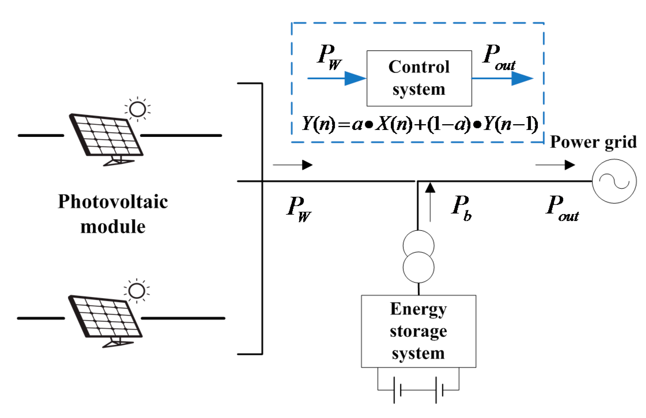
3.1. Smooth Control Principle of the First-Order Low-Pass Filter for Energy Storage Systems

The first-order low-pass filter (as shown in Figure 6) is used to smooth the fluctuation of the PV output power and the relationship between the energy storage capacity and the acquisition time internal of the data is analyzed.

The output of energy storage systems $P_b$ is obtained by Equation (9):

$$P_b=P_{out}-P_s$$

(9)

where $P_s$ is the output power of the PV module collected by the controller and $P_{out}$ is the power of PV connected to grid smoothed by the first-order low-pass filter.

The required capacity of energy storage systems E is calculated by Equation (10):

$$E={\displaystyle \underset{0}{\overset{T}{\int }}{P}_b}d\Delta$$

(10)

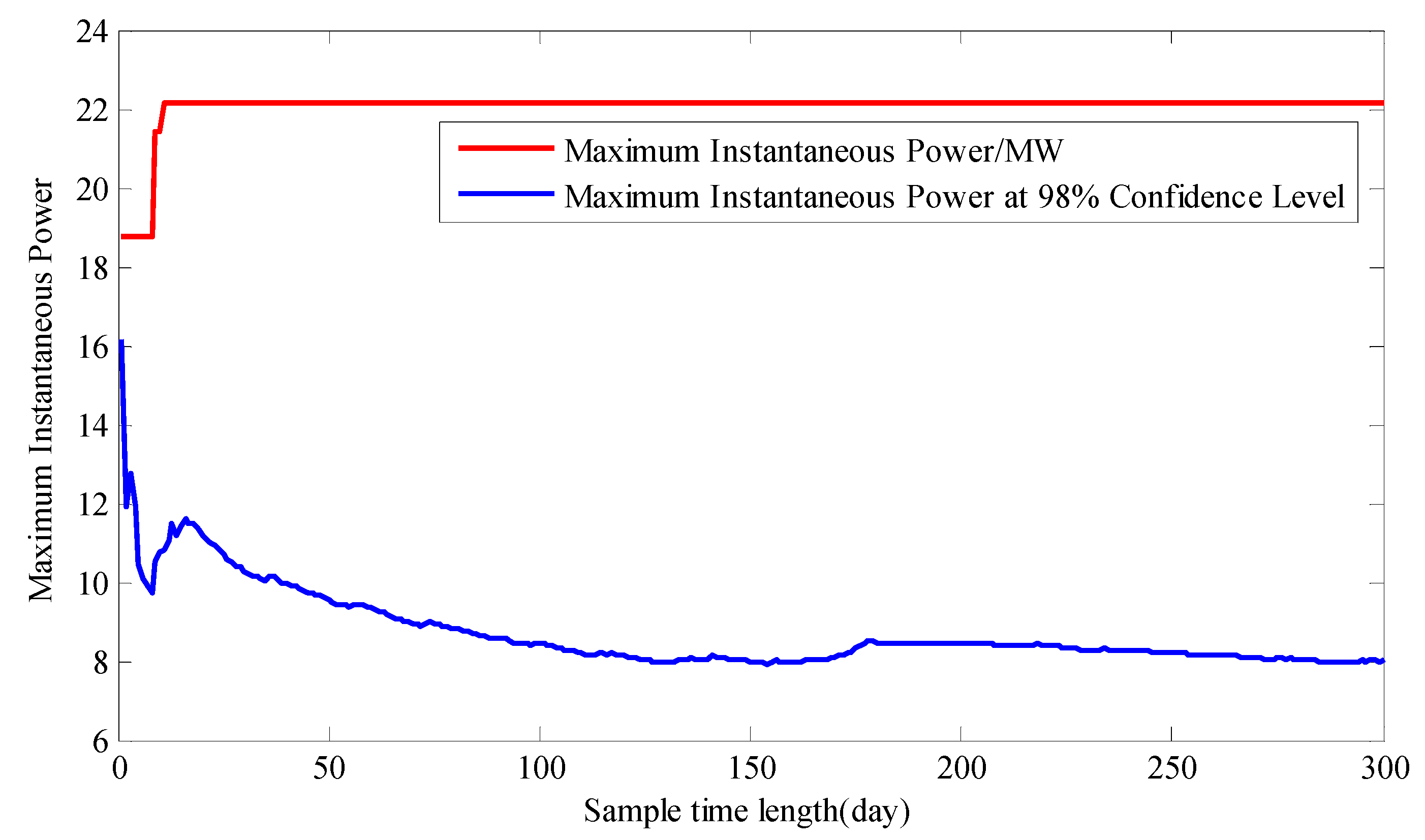
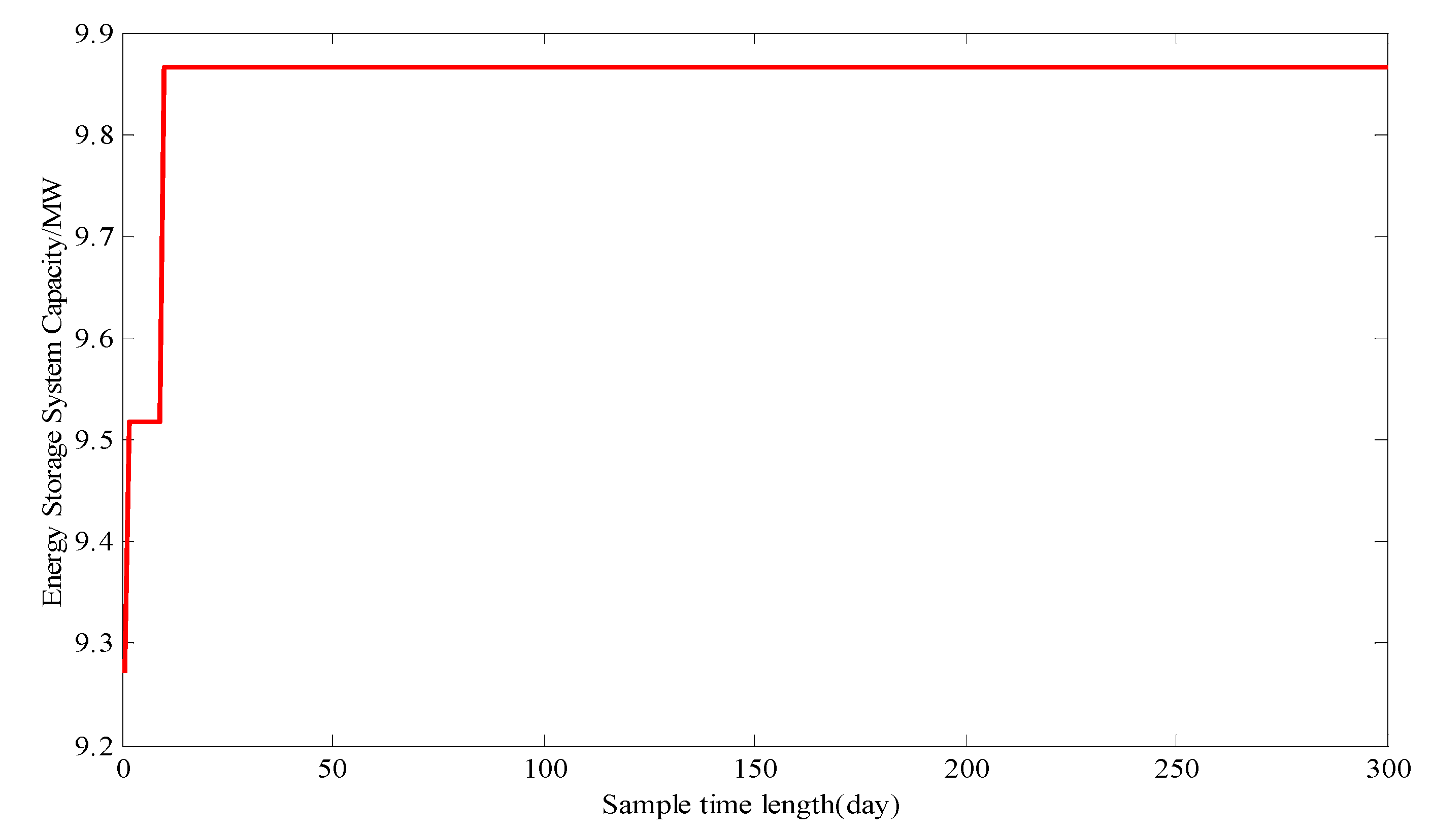
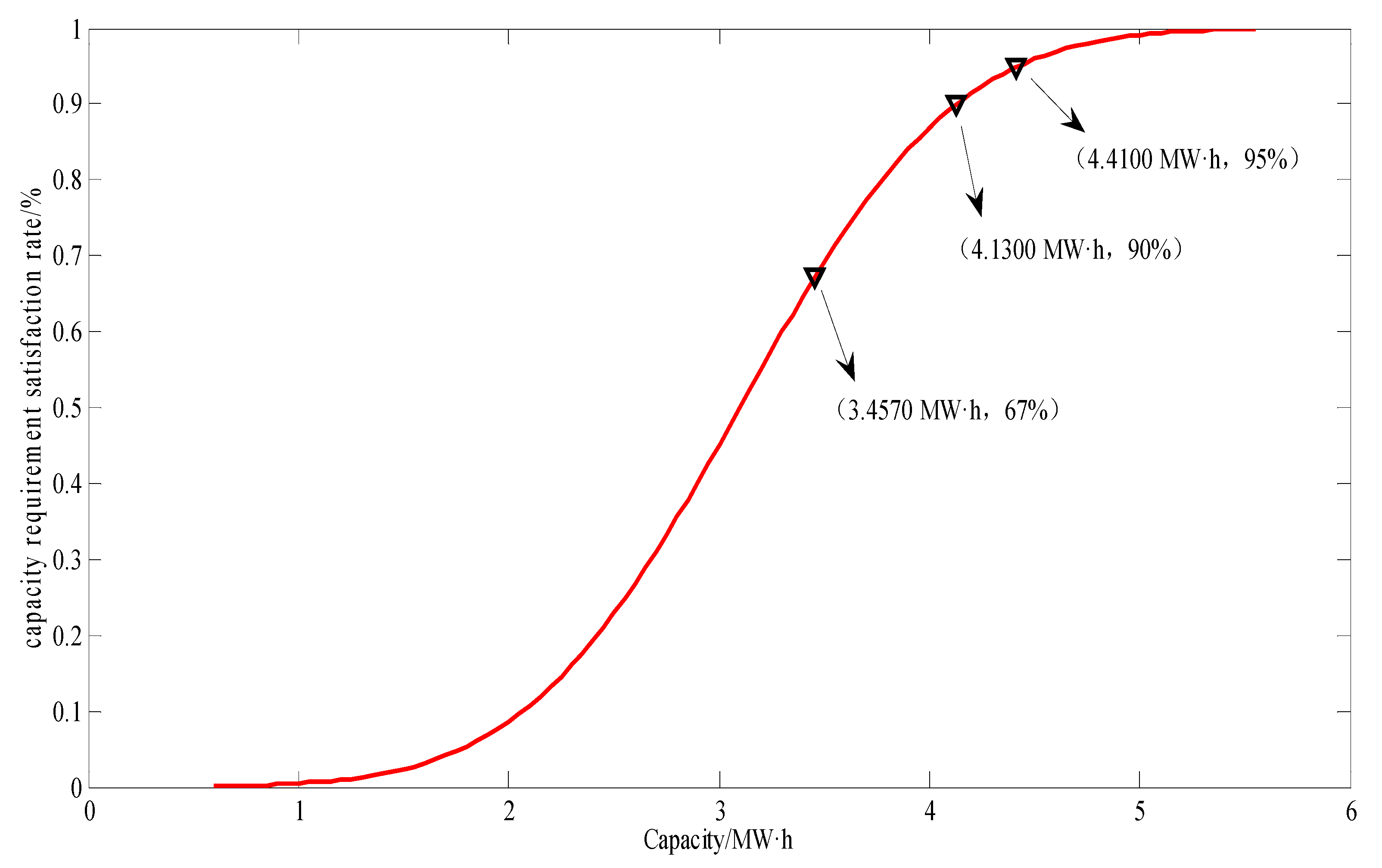
3.2. The Influence of the Sampling Time Length on the Capacity Configuration of Energy Storage Systems

Suppose the acquisition time internal of the PV output power is 60 s and 45 s, the sampling time length accumulates successively from the first day, and the capacity configuration results of the PV power station under different sampling time length are as shown in Figure 7 and Figure 8.

It can be seen from Figure 7 and Figure 8, that the required capacity and maximum instantaneous power of energy storage systems gradually increase before the sampling time length takes 30 days and remain stable after the sampling time length takes 30 days, after which it no longer continues to increase.

For the sake of generality, a total of 100 consecutive reorderings are made for successive output days and the number of days in the 300 samples to achieve the required maximum power and capacity after each reordering is recorded. The frequency distribution histogram and the normal distribution fit curve are shown in Figure 9.

From the fitting effect in Figure 9, when the output data time length of the PV power station is 21–25 days, the frequency of maximum power demand quantity is the most, that is, when we use the 21–25 days as the sample days, it is most probable to get the power of required energy storage system. When we use 23–26 days as the sample days, the frequency of occurrence of maximum capacity demand is the biggest, that is, when using 23–26 days as the sample days, it is most probable to get the required capacity of the energy storage system. Combining this with the conclusion of Section 2.4, when the allowable error accuracy is 0.3, the data time length is 23 days. Note that Figure 8 is the distribution statistics for 100 time random rankings. Therefore, the data length of PV data can be determined as 23 days, that is, randomly selecting the data 2, 3, 4, 6, 8 days from five weather types: sunny day, clear turning to cloudy, cloudy turning to clear, rainy and cloudy.

4. Comparison and Analysis of Capacity Configuration of the Energy Storage System

4.1. Configure Capacity based on One-Year Historical Data

Under application scenarios of stabilizing the power fluctuation of a PV power station, we take a PV power plant with an installed capacity of 40 MW as an example and record the PV power data for a time length of 360 days and the 360-day charge and discharge power of the energy storage system. Then we calculate the required energy storage capacity of the jth day:

$$Cap(j)=\max (N_1,N_2)$$

(11)

$$N_1=\max (|{\displaystyle \sum _{i=1}^k}{P}_{ji}\Delta t|),k=1,2,...,s$$

(12)

$$N_2=\max (|{\displaystyle \sum _{i=1}^{m_1}}{P}_{ji}\Delta t|,|{\displaystyle \sum _{i=m_2}^{m_3}}{P}_{ji}\Delta t|,...,|{\displaystyle \sum _{i=m_j}^{m_s}}{P}_{ji}\Delta t|)$$

(13)

where Cap(j) is the installed energy storage capacity of jth day (j = 1, 2, ..., 360), and P_ji is the charge/discharge power value at moment i of jth day, $\Delta t$ is the sampling interval and $1~m_1,m_2~m_3,m_j~m_n$ is data sampling moment of the energy storage uninterrupted charge/discharge.

We define the capacity demand satisfaction rate as a probability that storage system capacity value can meet the system capacity requirements:

$$F(x)=P(X\le x)$$

(14)

where X is the daily energy storage system capacity requirement, P is the probability of satisfying the capacity requirement and x is the maximum demand capacity under the capacity demand satisfaction rate P.

The relationship between the different storage capacity and the capacity demand satisfaction rate can be obtained from the cumulative distribution function (CDF) curve of Cap (j), as shown in Figure 10.

4.2. Configure Energy Storage Capacity Based on the Time Length Conclusion of PV Output Data

Aiming at a certain PV power plant with an installed capacity of 40 MW, bringing the power data which corresponds to the date time length determined in Section 2 into Equations (11)–(13), according to the calculation method in Section 4.1, when the capacity requirement satisfaction rate is 95%, the storage capacity is 4.4523 MW·h, which represent a 95% probability to meet the daily capacity requirements of the energy storage system, approaching the one-year configured energy storage capacity. Based on the same calculation method, when the installed capacity is 14 MW and 25 MW, we can obtain the corresponding storage capacities, as shown in

Table 3. Energy storage capacity allocation results under different installed capacity.

Installed Capacity/MW	14	25	40
Energy storage capacity/MW·h	1.5583	2.7827	4.4523

.

5. Conclusions

In this paper, firstly, a statistical analysis of the output data of a PV power plant is carried out and the periodic characteristics of the output data of the PV power plant are obtained by autocorrelation analysis. Seven kinds of characteristic weather parameters are selected to do cluster analysis on the PV output data and the total capacity space is decomposed into the capacity subspace of these five weather categories. Based on the statistical principle, the optimal sample capacity estimation of the PV output data under different weather categories is done. The required data time length at the time of analyzing PV output data of a PV plant whose time interval is 45 s and 60 s is determined, the relationship between the energy storage capacity and the data time length is investigated, the rationality of the length of the selected time is verified, meanwhile the capacity configuration of the energy storage system based on the optimal data time length is presented. The results show that when the time length of the PV output data is 23 days, it can meet the requirements of the data volume requirement to configure the storage capacity.

References

1. Pinto, R.; Mariano, S.; Calado, M.; de Souza, J. Impact of Rural Grid-Connected Photovoltaic Generation Systems on Power Quality. Energies 2016, 9, 739. [Google Scholar] [CrossRef]
2. Hong, Y.Y.; Lai, Y.M.; Chang, Y.R.; Lee, Y.D.; Liu, P.W. Optimizing Capacities of Distributed Generation and Energy Storage in a Small Autonomous Power System Considering Uncertainty in Renewables. Energies 2015, 8, 2473–2492. [Google Scholar] [CrossRef]
3. Alghamdi, A.; Bahaj, A.B.; Wu, Y. Assessment of Large Scale Photovoltaic Power Generation from Carport Canopies. Energies 2017, 10. [Google Scholar] [CrossRef]
4. Gulin, M.; Pavlović, T.; Vašak, M. A one-day-ahead photovoltaic array power production prediction with combined static and dynamic on-line correction. Sol. Energy 2017, 142, 49–60. [Google Scholar] [CrossRef]
5. Yadav, A.K.; Chandel, S.S. Identification of relevant input variables for prediction of 1-minute time-step photovoltaic module power using Artificial Neural Network and Multiple Linear Regression Models. Renew. Sustain. Energy Rev. 2017, 77, 955–969. [Google Scholar] [CrossRef]
6. Sichilalu, S.; Mathaba, T.; Xia, X. Optimal control of a wind–PV-hybrid powered heat pump water heater. Appl. Energy 2017, 185, 1173–1184. [Google Scholar] [CrossRef]
7. Chen, W.L.; Tsai, C.T. Optimal Balancing Control for Tracking Theoretical Global MPP of Series PV Modules Subject to Partial Shading. IEEE Trans. Ind. Electron. 2015, 62, 4837–4848. [Google Scholar] [CrossRef]
8. Abdelrazek, S.A.; Kamalasadan, S. Integrated PV Capacity Firming and Energy Time Shift Battery Energy Storage Management Using Energy-Oriented Optimization. IEEE Trans. Ind. Appl. 2016, 52, 2607–2617. [Google Scholar] [CrossRef]
9. Liu, G.Q.; Yuan, Y.; Wang, M.; Dai, X.; Xu, L. Energy storage capacity determining of PV plant considering economic cost. Renew. Energy Resour. 2014, 1, 1–5. [Google Scholar]
10. Zhu, L.; Yan, Z.; Yang, X.; Fu, Y.; Chen, J. Optimal configuration of battery capacity in microgrid composed of wind power and photovoltaic generation with energy storage. Power Syst. Technol. 2012, 12, 26–31. [Google Scholar]
11. Hu, G.Z.; Duan, S.X.; Cai, T.; Chen, C.S. Sizing and cost analysis of photovoltaic generation system based on vanadium redox battery. Trans. Chin. Electron. Soc. 2012, 5, 260–267. [Google Scholar]
12. Wu, X.G.; Liu, Z.Q.; Tian, L.T.; Ding, D.; Cheng, Z. Optimized capacity configuration of photovoltaic generation and energy storage device for stand-alone photovoltaic generation system. Power Syst. Technol. 2014, 5, 1271–1276. [Google Scholar]
13. Han, X.; Liu, D.; Liu, J.; Kong, L. Sensitivity analysis of PV output power to capacity configuration of energy storage systems from time and space characteristics. Int. J. Energy Res. 2017. [Google Scholar] [CrossRef]
14. Han, Z.H.; Zhu, X.X. Selection of training sample length in support vector regression based on information entropy. Proc. CSEE 2010, 20, 112–116. [Google Scholar]
15. Gao, P.X. Parametric modeling sample size selection. J. Vib. Meas. Diagn. 1991, 4, 9–14. [Google Scholar]
16. Shi, L.D.; Zhang, J.G.; Huang, S.Q. Investigating of random sample to determine the length of the data processing problem. Constr. Mach 1993, 4, 16–21. [Google Scholar]
17. Heck, D.W.; Moshagen, M.; Erdfelder, E. Model selection by minimum description length: Lower-bound sample sizes for the Fisher information approximation. J. Math. Psychol. 2014, 60, 29–34. [Google Scholar] [CrossRef]
18. Vallejos, R.; Osorio, F. Effective sample size of spatial process models. Spat. Stat. 2014, 9, 66–92. [Google Scholar] [CrossRef]
19. Chun, Y.; Griffith, D.A. A quality assessment of eigenvector spatial filtering based parameter estimates for the normal probability model. Spat. Stat. 2014, 10, 1–11. [Google Scholar] [CrossRef]
20. Rodrigues, E.M.G.; Godina, R.; Pouresmaeil, E.; Ferreira, J.R.; Catalão, J.P.S. Domestic appliances energy optimization with model predictive control. Energy Convers. Manag. 2017, 142, 402–413. [Google Scholar] [CrossRef]
21. Oliveira, D.; Rodrigues, E.M.G.; Mendes, T.D.P.; Catalão, J.P.S.; Pouresmaeil, E. Model predictive control technique for energy optimization in residential appliances. In Proceedings of the IEEE International Conference on Smart Energy Grid Engineering, Oshawa, ON, Canada, 17–19 August 2015; pp. 1–6. [Google Scholar]
22. Godina, R.; Rodrigues, E.M.G.; Pouresmaeil, E.; Matias, J.C.O.; Catalão, J.P.S. Model predictive control technique for energy optimization in residential sector. In Proceedings of the IEEE International Conference on Environment and Electrical Engineering, Florence, Italy, 7–10 June 2016. [Google Scholar]
23. Oliveira, D.; Rodrigues, E.M.G.; Godina, R.; Mendes, T.D.P.; Catalão, J.P.S.; Pouresmaeil, E. Enhancing home appliances energy optimization with solar power integration. In Proceedings of the IEEE Region 8 International Conference on Computer as a Tool (EUROCON), Salamanca, Spain, 8–11 September 2015. [Google Scholar]
24. Oliveira, D.; Rodrigues, E.M.G.; Godina, R.; Matias, J.C.O.; Catalão, J.P.S.; Pouresmaeil, E. MPC weights tunning role on the energy optimization in residential appliances. In Proceedings of the Power Engineering Conference, Wollongong, Australia, 27–30 September 2015; pp. 1–6. [Google Scholar]
25. Han, X.; Liu, D.; Liu, J.; Kong, L. Sensitivity analysis of acquisition granularity of photovoltaic output power to capacity configuration of energy storage systems. Appl. Energy 2017, 203, 794–807. [Google Scholar] [CrossRef]
26. Luo, B.; Yu, H.; Zhang, X.; Shen, Z.; Li, Q. On eigen-based signal combining using the autocorrelation coefficient. IET Commun. 2013, 6, 3091–3097. [Google Scholar] [CrossRef]
27. Zárate-Miñano, R.; Milano, F. Construction of SDE-based wind speed models with exponentially decaying autocorrelation. Renew. Energy 2016, 94, 186–196. [Google Scholar] [CrossRef]
28. Bhandary, M. On confidence interval of a common autocorrelation coefficient of two populations in multivariate data when the errors are autocorrelated. J. Stat. Manag. Syst. 2016, 19, 509–517. [Google Scholar] [CrossRef]
29. Saygin, D.; Kempener, R.; Wagner, N.; Ayuso, M.; Gielen, D. The Implications for Renewable Energy Innovation of Doubling the Share of Renewables in the Global Energy Mix between 2010 and 2030. Energies 2015, 8, 5828–5865. [Google Scholar] [CrossRef]
30. Brenna, M.; Dolara, A.; Foiadelli, F.; Lazaroiu, G.C.; Leva, S. Transient Analysis of Large Scale PV Systems with Floating DC Section. Energies 2012, 5, 3736–3752. [Google Scholar] [CrossRef]
31. Fu, G.; Fu, J.; Xu, Y.; Chen, Z.; Lai, J. Accuracy enhancement of five-axis machine tool based on differential motion matrix: Geometric error modeling, identification and compensation. Int. J. Mach. Tools Manuf. 2015, 89, 170–181. [Google Scholar] [CrossRef]
Figure 1. The output level of each month of PV power plant.
Energies 10 01616 g001
Figure 2. Autocorrelation coefficient of PV output data. (a) 96-h autocorrelation coefficient and (b) 2400-h autocorrelation coefficient.
Energies 10 01616 g002
Figure 3. Typical output curves under five different types of weather.
Energies 10 01616 g003
Figure 4. Clustering analysis on PV data based on weather conditions (one part).
Energies 10 01616 g004
Figure 5. Optimal sample capacity estimation.
Energies 10 01616 g005
Figure 6. Schematic diagram of the first-order low-pass filter control algorithm for energy storage systems.
Energies 10 01616 g006
Figure 7. The relationship between the required maximum instantaneous power of energy storage systems and sampling time length.
Energies 10 01616 g007
Figure 8. The relationship between the required capacity of energy storage systems and sampling time length.
Energies 10 01616 g008
Figure 9. The frequency distribution of the sampling time length reaching to the demand of energy storage systems. (a) The required maximum power corresponding to the sampling time length; (b) The required maximum capacity corresponding to the sampling time length.
Energies 10 01616 g009
Figure 10. The relationship between annual storage capacity and capacity demand satisfaction rate.
Energies 10 01616 g010