Article

Short-Term Electricity-Load Forecasting Using a TSK-Based Extreme Learning Machine with Knowledge Representation

Department of Control and Instrumentation Engineering, Chosun University, Gwangju 61452, Korea
*
Author to whom correspondence should be addressed.
Energies 2017, 10(10), 1613; https://doi.org/10.3390/en10101613
Submission received: 25 September 2017 / Revised: 9 October 2017 / Accepted: 10 October 2017 / Published: 16 October 2017
(This article belongs to the Section F: Electrical Engineering)

Abstract

:
This paper discusses short-term electricity-load forecasting using an extreme learning machine (ELM) with automatic knowledge representation from a given input-output data set. For this purpose, we use a Takagi-Sugeno-Kang (TSK)-based ELM to develop a systematic approach to generating if-then rules, while the conventional ELM operates without knowledge information. The TSK-ELM design includes a two-phase development. First, we generate an initial random-partition matrix and estimate cluster centers for random clustering. The obtained cluster centers are used to determine the premise parameters of fuzzy if-then rules. Next, the linear weights of the TSK fuzzy type are estimated using the least squares estimate (LSE) method. These linear weights are used as the consequent parameters in the TSK-ELM design. The experiments were performed on short-term electricity-load data for forecasting. The electricity-load data were used to forecast hourly day-ahead loads given temperature forecasts; holiday information; and historical loads from the New England ISO. In order to quantify the performance of the forecaster, we use metrics and statistical characteristics such as root mean squared error (RMSE) as well as mean absolute error (MAE), mean absolute percent error (MAPE), and R-squared, respectively. The experimental results revealed that the proposed method showed good performance when compared with a conventional ELM with four activation functions such sigmoid, sine, radial basis function, and rectified linear unit (ReLU). It possessed superior prediction performance and knowledge information and a small number of rules.

1. Introduction

The electric power system is often considered the most complex system devised by humans. It consists of dynamic components, including transformers, generators, transmission and distribution lines, nonlinear and linear loads, protective devices, etc. These components must operate synergistically in a manner that ensures the stability and reliability of the electric power system during disturbances.
An important aspect of electric-power system operation is that the system performance follows the load requirements. An individual decrease or increase in power generation depends on a respective decrease or increase in the system load. The electric utility operator allocates the system resources through prior knowledge of the load requirements. The ability to forecast electricity-load requirements plays an important role in providing effective power-system management [1]. Thus, accurate electricity-load forecasting is critical for short-term operations and long-term planning for every electric utility. The electricity-load forecasting system influences several decisions, including which generators to commit for a given period [2].
Over the past few decades, many studies have been conducted on short-term electricity-load forecasting. Dong [3] proposed a forecasting method model using data decomposition approach for short-term electricity load forecasting. Huang [4] proposed a permutation importance-based feature-selection method for short-term electricity-load forecasting using the random forest learning method. The original feature set was used to train random forest as the original model. Bennett [5] proposed a combined model using an autoregressive integrated moving average with exogenous variables and a neural network with back-propagation (BP) learning for the short-term load forecast of low-voltage residential distribution networks. Hernandez [6] proposed an electric-load forecast architectural model based on Multi-Layer Perceptron neural networks for microgrids. Amjady [7] proposed a new neural network approach to short-term load forecasting. The proposed network was based on a modified harmony search technique, which can avoid the overfitting problem and being trapped in local minima. Goude [8] proposed local short- and middle-term electricity-load forecasting with semi-parametric additive models to model the electrical load of over 2200 substations in the French distribution network. Guo [9] proposed accelerated continuous conditional random fields that can treat a multi-steps-ahead regression task as a sequence-labeling problem for load forecasting. Yu [10] proposed a sparse coding approach to household electricity-load forecasting in smart grids. The proposed methods were tested on a data set of 5000 households in a joint project with the electric power board of Chattanooga, Tennessee. Chen [11] proposed a support-vector regression model to calculate the demand-response baseline for short-term electrical-load forecasting of office buildings. Ren [12] proposed a random-vector functional-link network for short-term electricity-load demand forecasting. Lopez [13] proposed a combined model based on a wavelet neural network, particle swarm optimization, and an ensemble empirical-mode decomposition.
Other studies have focused on extreme learning machines (ELMs) with fast learning using the LSE, in contrast to the traditional neural networks with BP learning schemes in previous literature. ELMs are feed forward neural networks for classification or regression with a single layer of hidden nodes. The weights connecting the inputs to the hidden nodes are randomly assigned and never updated. They are learned in a single step, which essentially amounts to learning the linear weights.
Zhang [14] performed short-term load forecasting of the Australian National electricity market with an ensemble ELM model based on the ensemble learning strategy. Golestaneh [15] performed very short-term nonparametric probabilistic forecasting of renewable energy generation with applications to solar energy, using ELMs as a fast regression model. Li [16] proposed a novel wavelet-based ensemble method for short-term load forecasting with hybrid neural networks and feature selection. A wavelet-based ensemble scheme was employed to generate the individual ELM-based forecasters. Cecati [17] proposed a novel radial basis function (RBF) training method for short-term electric-load forecasting and comparative studies including ELMs. Li [18] proposed a hybrid short-term electric-load forecasting strategy base d on a wavelet transform, an ELM, and a modified artificial bee-colony algorithm. Yang [19] proposed a hybrid approach that combines the wavelet transform and a kernel ELM, based on self-adapting particle-swarm optimization. Li [20] proposed an ensemble method for short-term load forecasting based on a wavelet transform, an ELM, and partial least squares regression.
Although these ELM methods have demonstrated their prediction and classification superiority, it is difficult to obtain meaningful information. Therefore, we propose a new ELM predictor with knowledge representation, e.g., if-then rules, for short-term electricity-load forecasting. For this, a TSK-based ELM is proposed as a systematic approach to generating fuzzy if-then rules.
The TSK-ELM design includes a two-phase development. First, we generate an initial random-partition matrix and estimate the cluster centers. This is similar to generating random weights between the input and hidden layers in the original ELM design [21]. The obtained cluster centers are used as the premise parameters of the fuzzy if-then rules. Next, the TSK-type linear weights are estimated by LSE. These linear weights are used as the consequent parameters. The electricity-load data are used to forecast hourly day-ahead loads, given temperature forecasts, holiday information, and historical loads from the New England Power Pool region [22,23].
This paper is organized in the following manner. Section 2 describes the architecture and concept of conventional ELM as an intelligent predictor. Section 3 describes the design method of a TSK-based ELM with knowledge representation for short-term electricity-load forecasting. Section 4 covers the performance measure and simulation results from the electricity-load data. Finally, concluding comments are presented in Section 5.

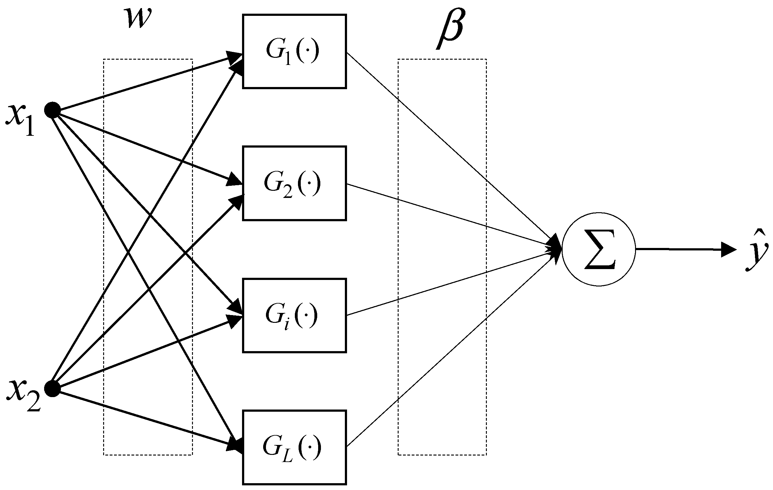
2. ELM as an Intelligent Predictor

Conventional studies on neural networks have focused on learning and adaptation for classification and regression. Several studies have been investigated the development of good learning methods in the past decades. In contrast to well-known neural networks, e.g., the multilayer perceptron (MLP) and radial basis function network (RBFN), ELMs possess a real-time learning capability and good prediction ability as intelligent predictors [21,24,25].
Figure 1 shows the architecture of an ELM predictor. Given random hidden neurons, which need not be an algebraic sum or other ELM feature mappings, almost any nonlinear piecewise continuous hidden nodes can be represented as follows [21]:
H i ( x ) = G i ( w i , b i , x )
where w i and b i are the weights and biases between the input layer and the hidden layer, respectively.
The output function of a generalized single layer feedforward network (SLFN) is expressed as
f L ( x ) = i = 1 L β i G i ( w i , b i , x )
The output function in the hidden-layer mapping is as follows:
H ( x ) = [ G 1 ( w 1 , b 1 , x ) , , G L ( w L , b L , x ) ]
The output functions of the hidden nodes can be used by the various forms. The different types of activation function include sigmoid networks, RBF networks, polynomial networks, complex networks, sine function, ReLU, and wavelet networks, some of which are described as follows:
Sigmoid :   G ( w i , b i , x ) = 1 1 + e ( w i x + b i )
RBF :   G ( w i , b i , x ) = e ( w i x + b i ) 2
Sine :   G ( w i , b i , x ) = sin ( w i x + b i )
ReLU :   G ( w i , b i , x ) = max ( w i x + b i , 0 )
where G ( w , b , x ) and L are the output function of hidden node and the number of hidden node, respectively.
In what follows, we shall review the processing procedure of an ELM predictor. ELM determines output weights using the following steps:
  • Randomly assign hidden node parameters ( w i , b i ) , i = 1 , 2 , , N .
  • Calculate the hidden-layer output matrix H = [ h ( x 1 ) h ( x N ) ] .
  • Calculate the output weights β using a LSE:
    β = Η * T
where H * is the Moore–Penrose generalized inverse of matrix H . T is the target output vector. When H T H is nonsingular, H * = ( H T H ) 1 H T is the pseudo-inverse of H. This is a standard LSE problem and the best solution for β is expressed as follows:
β = ( H T H ) 1 H T T
We can develop ELM by adding a positive value to the diagonal of H T H with the use of the ridge regression. By doing this, the resultant prediction can obtain better generalization performance [26]. The essence of an ELM can be summarized by the following features. First, the hidden layer does not need to be tuned. Second, the hidden layer mapping h(x) satisfies the universal approximation conditions [24]. Next, the ELM parameters are estimated to minimize, as follows:
H β T 2

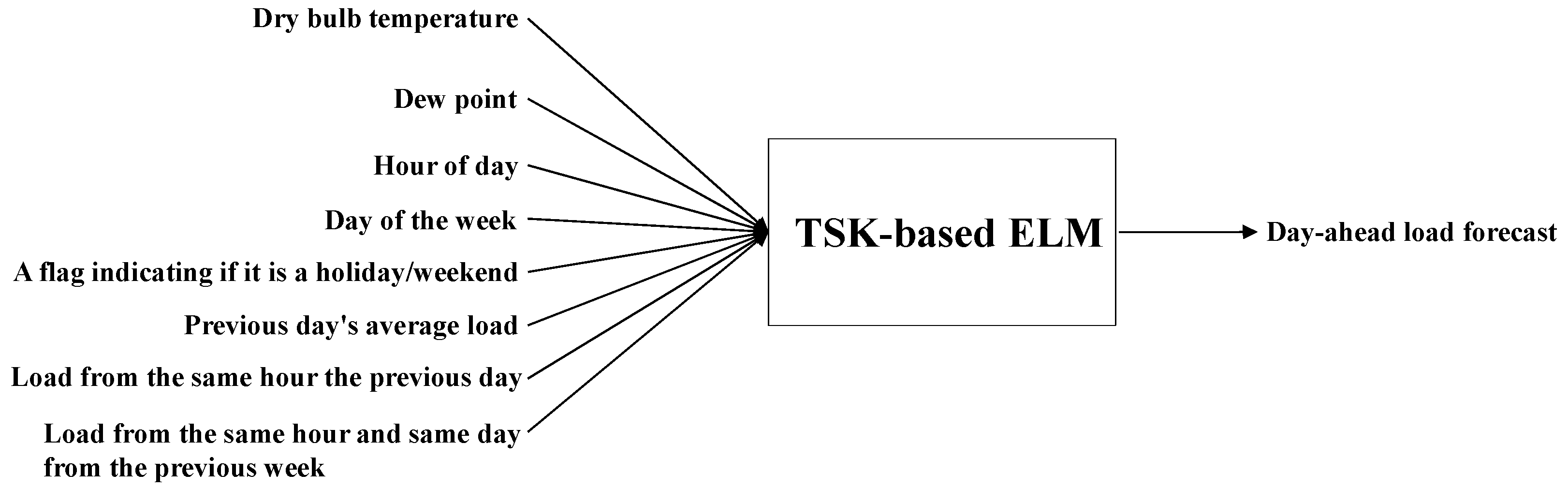
3. Design of TSK-Based ELM for Short-Term Electricity-Load Forecasting

In this section, we describe a new ELM predictor with knowledge information obtained from TSK-based rules for short-term electricity-load forecasting.

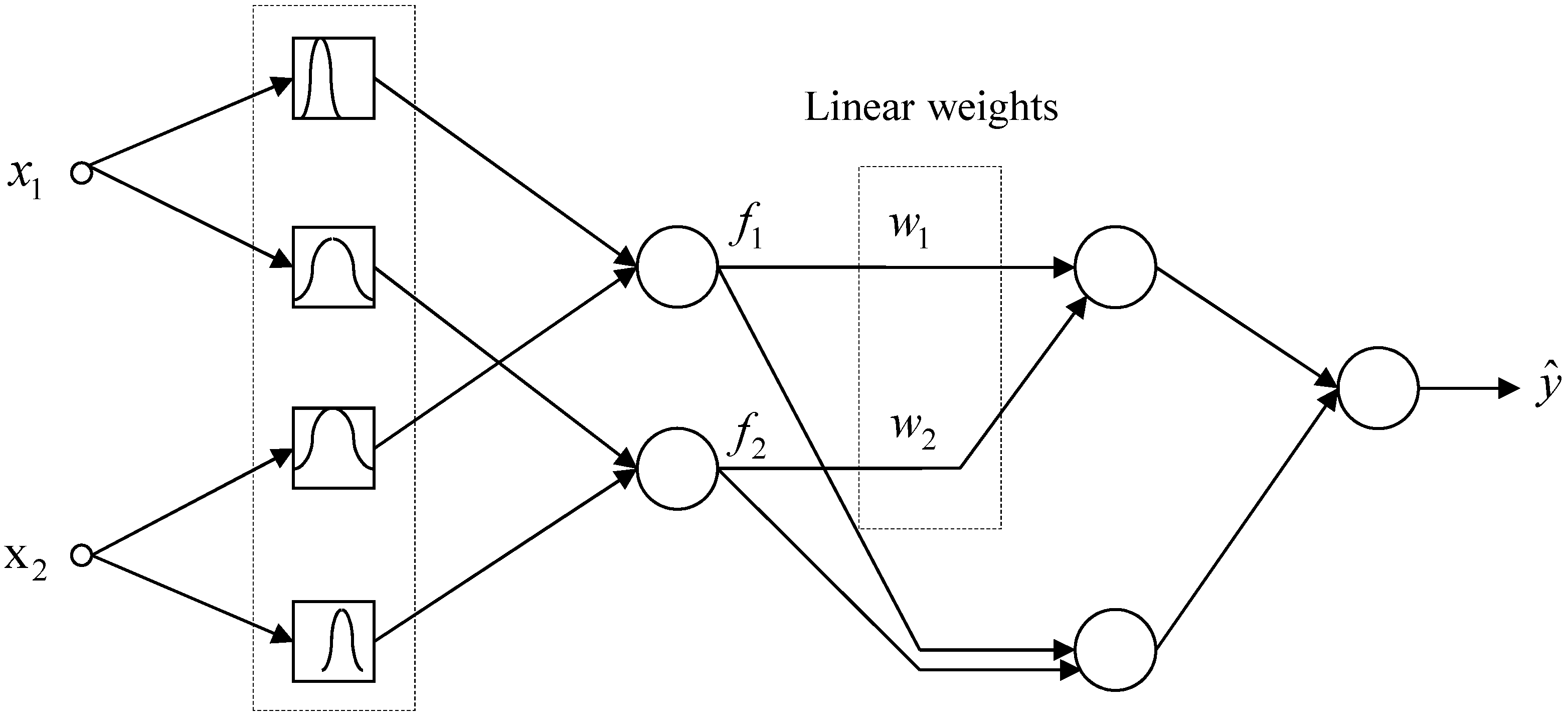
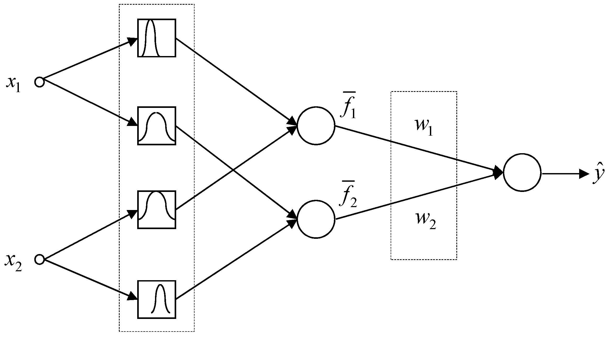
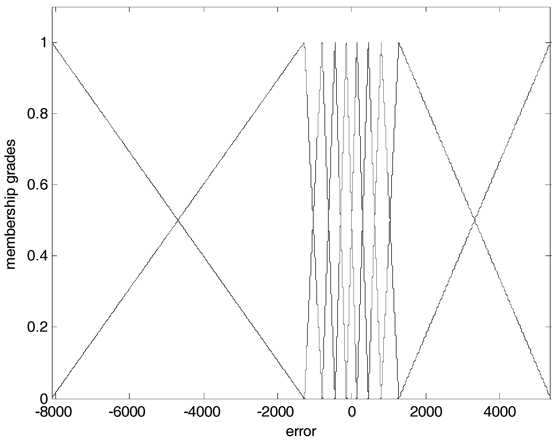
3.1. TSK-ELM Architecture and Knowledge Representation

The proposed TSK-ELM is an innovative approach to constructing a computationally intelligent predictor. This predictor can automatically extract knowledge information from a numerical input-output data set. The knowledge is represented by TSK-type fuzzy rules, in which the consequent part is a polynomial in the input variables. Although the conventional ELM predictor shows good prediction performance with a single forward pass, it is difficult to extract and represent the knowledge information.
In the following, we shall explain the architecture and each layer of the proposed TSK-ELM. For simplicity, we suppose that the TSK-ELM to be considered has two inputs x 1 and x 2 and one output. The TSK-type rule set is expressed in the following form:
If   x 1   is   A i   and   x 2   is   B i ,   then   w i = p i x 1 + q i x 2 + r i .
This rule is composed of the premise part and the consequent part. Figure 2 shows the architecture of the TSK-ELM predictor. The network consists of four layers. The nodes of the first layer are obtained by random clustering. We generate an initial random partition matrix and estimate the cluster centers. This process is very similar to the concept of generating random weights between the input and hidden layer in the original ELM design [21]. The obtained cluster centers are used as the premise parameters for the fuzzy if-then rules.
The membership function is characterized by a Gaussian membership function, which is specified by two parameters as follows:
μ A ( x ) = e 1 2 ( x c σ ) 2
A Gaussian membership function is determined by cluster center c and width σ . Each cluster center c i is obtained by an initial random partition matrix u i j as follows:
c i = j = 1 n u i j m x j j = 1 n u i j m
μ i j = 1 k = 1 c ( d i j d k j ) 2 / ( m 1 )
where u i j is between 0 and 1. d i j = c j x j is the Euclidean distance between i-th cluster center and j-th data point. m [ 1 , ) is a weighting exponent.
The width σ j of each input variable is obtained by a statistical data distribution as follows:
σ j = α x max x min 2 2
where x max and x min are the maximum and minimum values in each input variable dimension, respectively. The fuzzy set A is a linguistic label and specifies the degree to which the given input satisfies the quantifier. These parameters are referred to as premise parameters. In the second layer, the output is the product of all the incoming signals and represents as the firing strength f i of a rule. The output of the third layer is obtained by a combination of the firing strength of a rule and the linear weights w i . Here, the consequent parameters are estimated by LSE, i.e., the same method as in the ELM design [21]. The single node in the final layer computes the overall output as the summation of all incoming signals, as follows:
y ^ = i = 1 r f i w i i = 1 r f i = i = 1 r f i ( p i x 1 + q i x 2 + r i ) i = 1 r f i
In what follows, we shall present more simplified structure than that of Figure 2. Figure 3 shows the simplified architecture of TSK-ELM as ELM structure. This network consists of three layers. Each node in the second layer represents the normalized firing strength f ¯ i of the rule. The weights between the second layer and third layer can be expressed by a constant or linear equation. The overall output was calculated by the linear combination of the consequent part and the weights. The linear combination are expressed as follows
y ^ = f ¯ 1 w 1 + f ¯ 2 w 2 = ( f ¯ 1 x 1 ) p 1 + ( f ¯ 1 x 2 ) q 1 + ( f ¯ 1 ) r 1 + ( f ¯ 2 x 1 ) p 2 + ( f ¯ 2 x 2 ) q 2 + ( f ¯ 2 ) r 2
The TSK-ELM structure can be viewed as the integration of adaptive neuro-fuzzy inference system (ANFIS) and ELM. In the structural aspect, the TSK-ELM is similar to that of ANFIS. In the case of conventional ANFIS with grid partition, it encounters the curse of dimensionality problem when have a moderately large number of inputs, while we use scatter partition method using random clustering with initial random partition matrix. Furthermore, in the theoretical aspect, we follow the main concept of the conventional ELM. Thus, we use an initial random-partition matrix and estimate cluster centers for random clustering. As for the width of Gaussian membership function, we obtain statistical values from Equation (10) without the assignment of random values. These cluster centers are used as the premise parameters of fuzzy if-then rules. The linear weights of the TSK fuzzy type are obtained using LSE. Recently, the initial random-partition method has been demonstrated the effectiveness in [27].

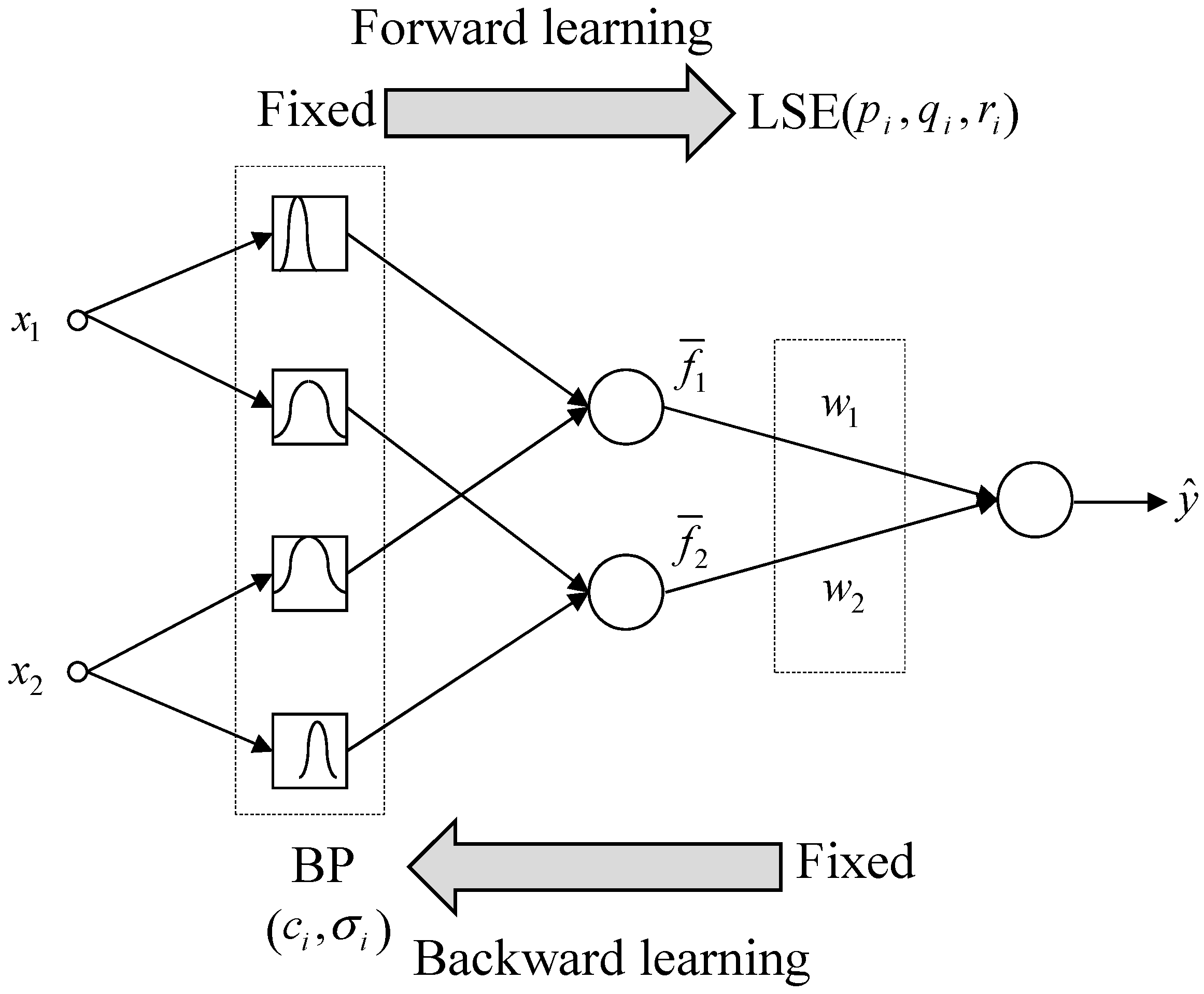
3.2. TSK-ELM’s Fast Learning and Hybrid-Learning

The consequent parameters are estimated by LSE to obtain the optimal parameters in the same manner as ELM. This process is achieved by one pass, based on LSE. To obtain better prediction performance, a hybrid-learning algorithm that combines BP and LSE for fast parameter identification can be applied directly.
Figure 4 shows a diagram of the hybrid-learning method in the TSK-ELM design. In the forward pass, the input values go forward until the second layer, and the consequent parameters are estimated by LSE. In the backward pass, the error signals propagate backward, and the premise parameters are updated by the BP method. The hybrid approach converges much faster, since it reduces the search space dimensions of the original BP method. Although we can apply BP to tune the parameters in the TSK-ELM design, this simple optimization method usually takes a long time before it converges. If the input-output data set is large, then the premise and consequent parameters should be fine-tuned. Human-determined parameters are seldom optimal in terms of reproducing the desired output. This learning scheme is equally applicable to RBFN. Furthermore, this hybrid-learning method using LSE and BP is the well-known scheme in the ANFIS design [28].

4. Experimental Results

In this section, we report on the comprehensive experiment set and describe comparative experiments to evaluate the performance of the proposed TSK-ELM for short-term electricity load forecasting.

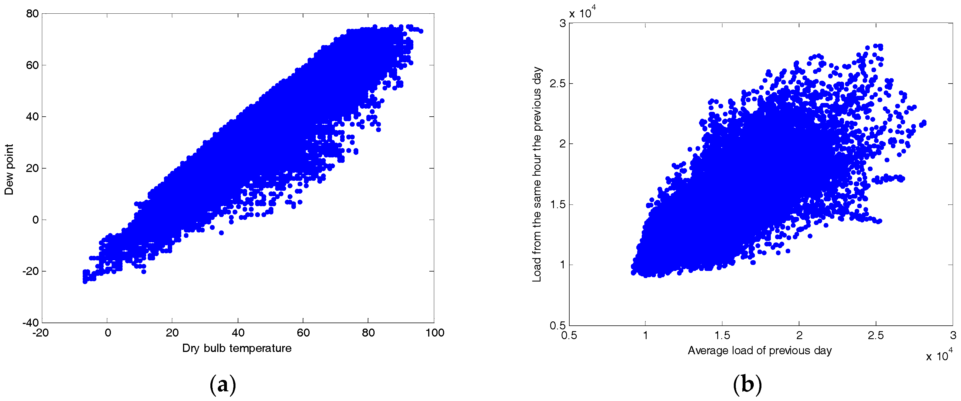
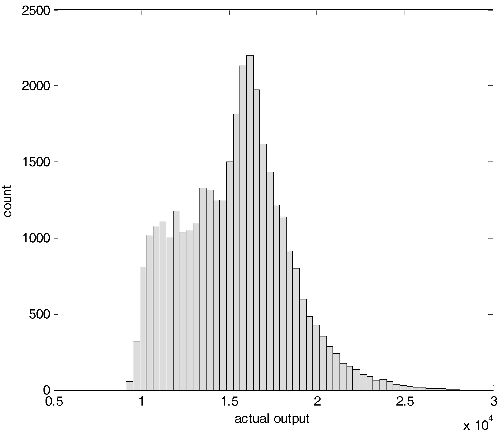
4.1. Training and Testing Data Sets

The input variables used in this example are dry bulb temperature, dew point, hour of day, day of the week, a flag indicating if it is a holiday/weekend, previous day’s average load, load from the same hour the previous day, and load from the same hour and same day from the previous week as shown in Figure 5. This example demonstrates building and validating a short-term electricity-load forecasting model. The model considers multiple information sources, including temperatures and holidays, when constructing a day-ahead load forecaster. The original data were obtained from the Zonal hourly load data websites of the New England ISO [22,23].
The numbers of training and testing data points are 35,068 from 2004 to 2007 and 8784 from 2008, respectively. The training data set is used for designing the TSK-ELM, while the testing data set is used for validating the generalization performance.
Since most similarity metrics are sensitive to the ranges of elements in the input vectors, each of the input variables must be normalized to within the unit interval [0, 1] except for out variable. For short-term forecasting, these include the dry-bulb temperature, dew point, hour of the day, day of the week, holiday and weekend indicators, the previous day’s average load, the load from the same hour the previous day, and the load from the same hour and same day of the previous week. Figure 6 visualizes the data distribution between input variables. Figure 7 shows a histogram of the actual output.

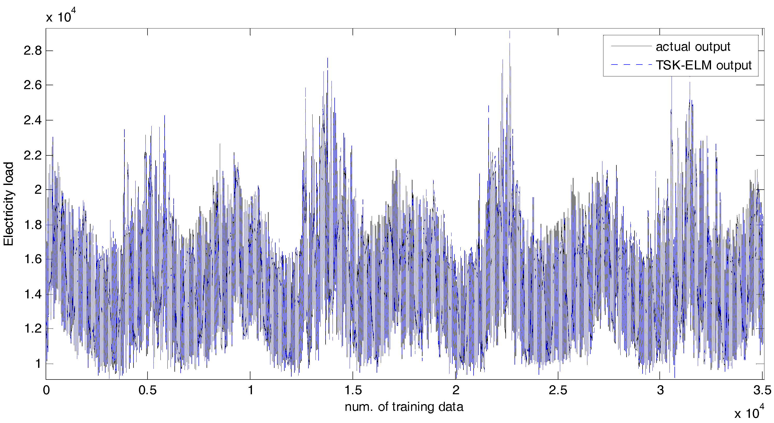
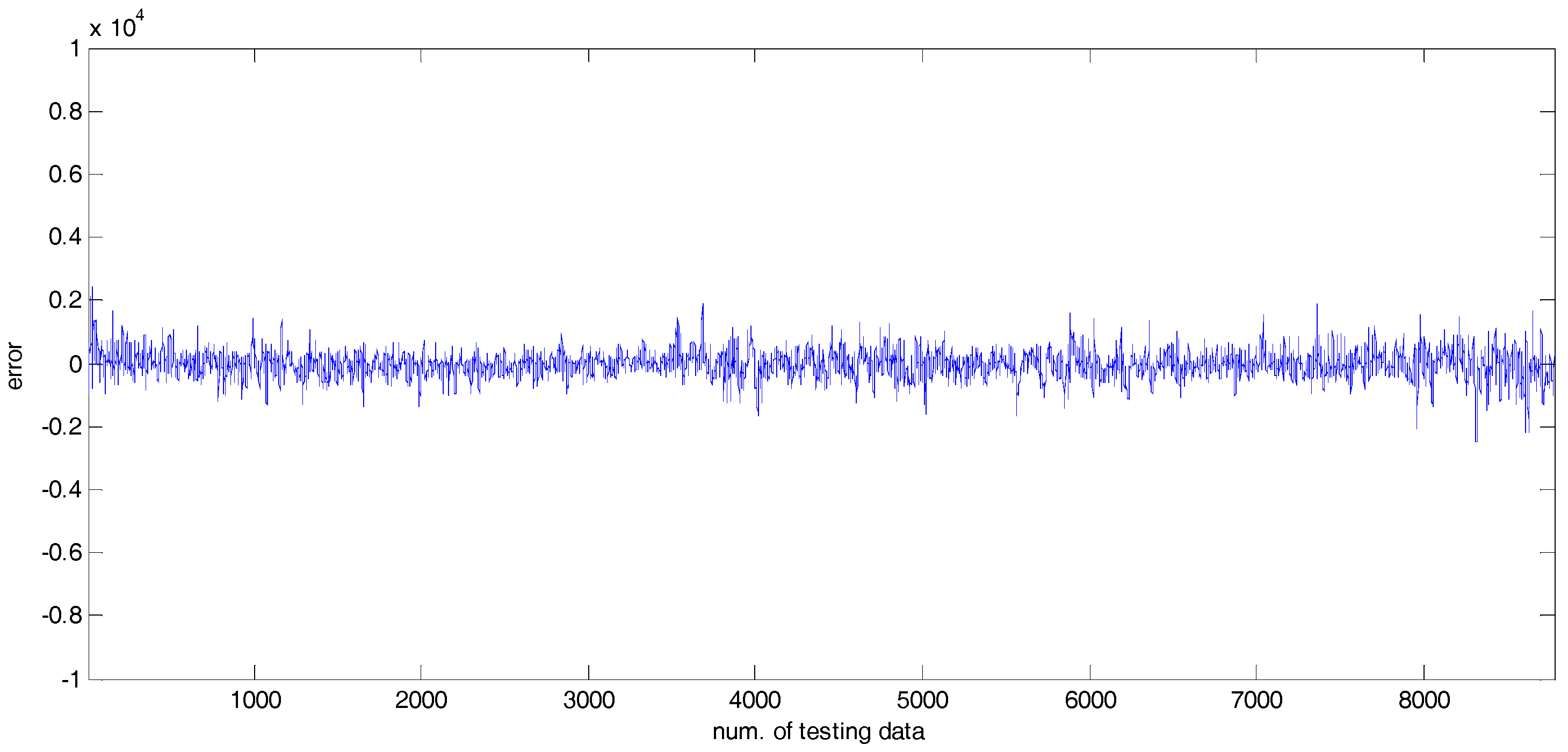
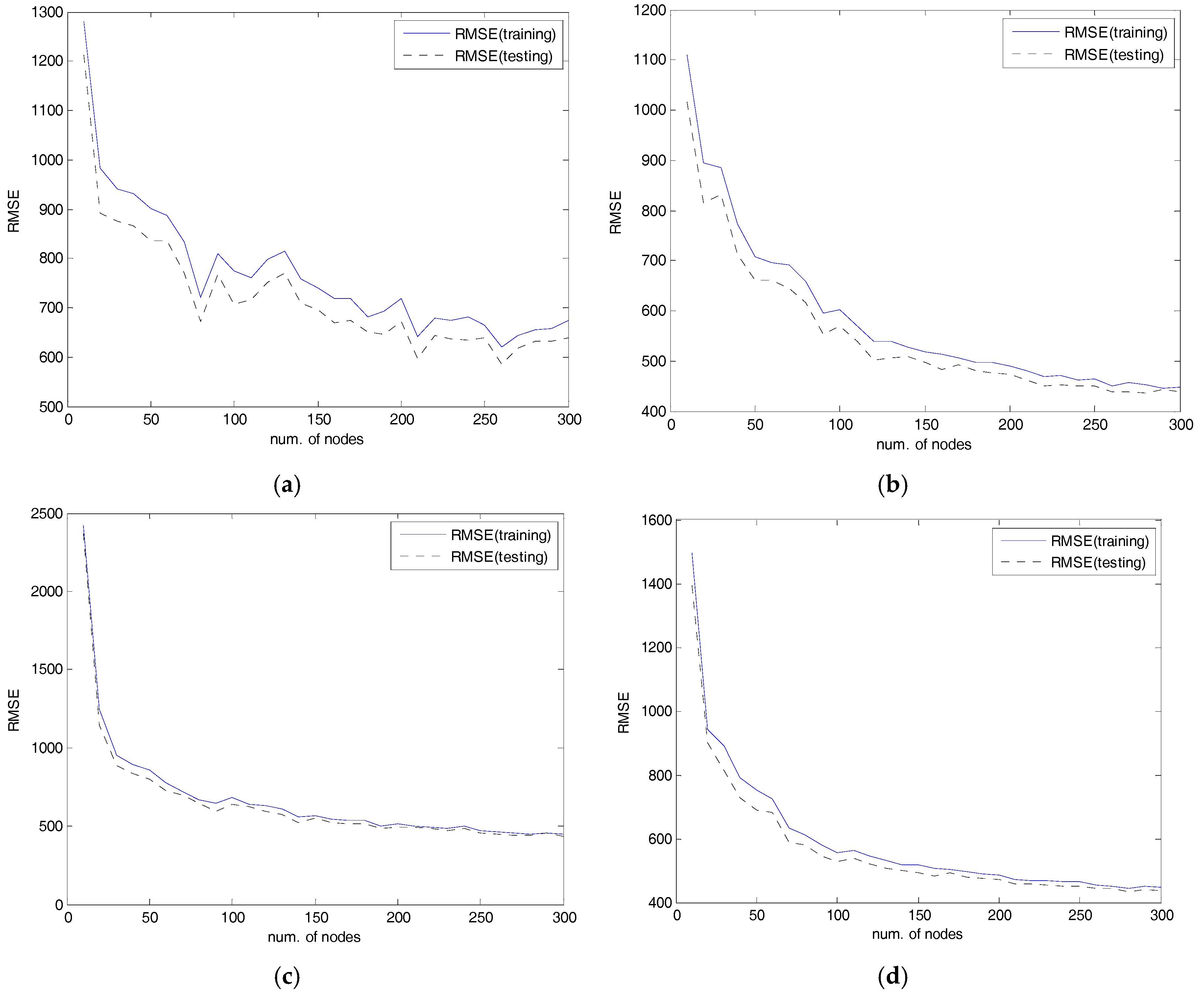
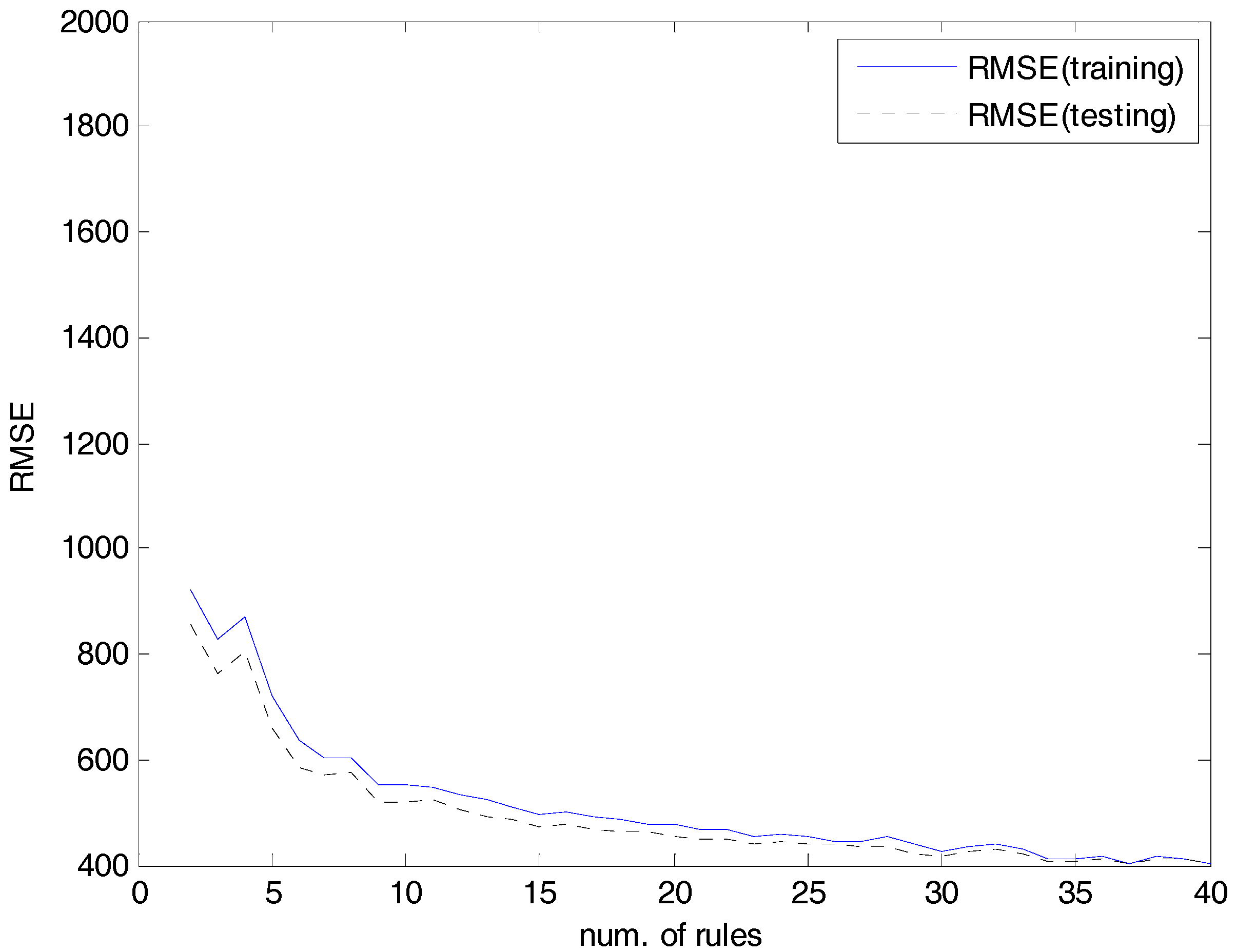
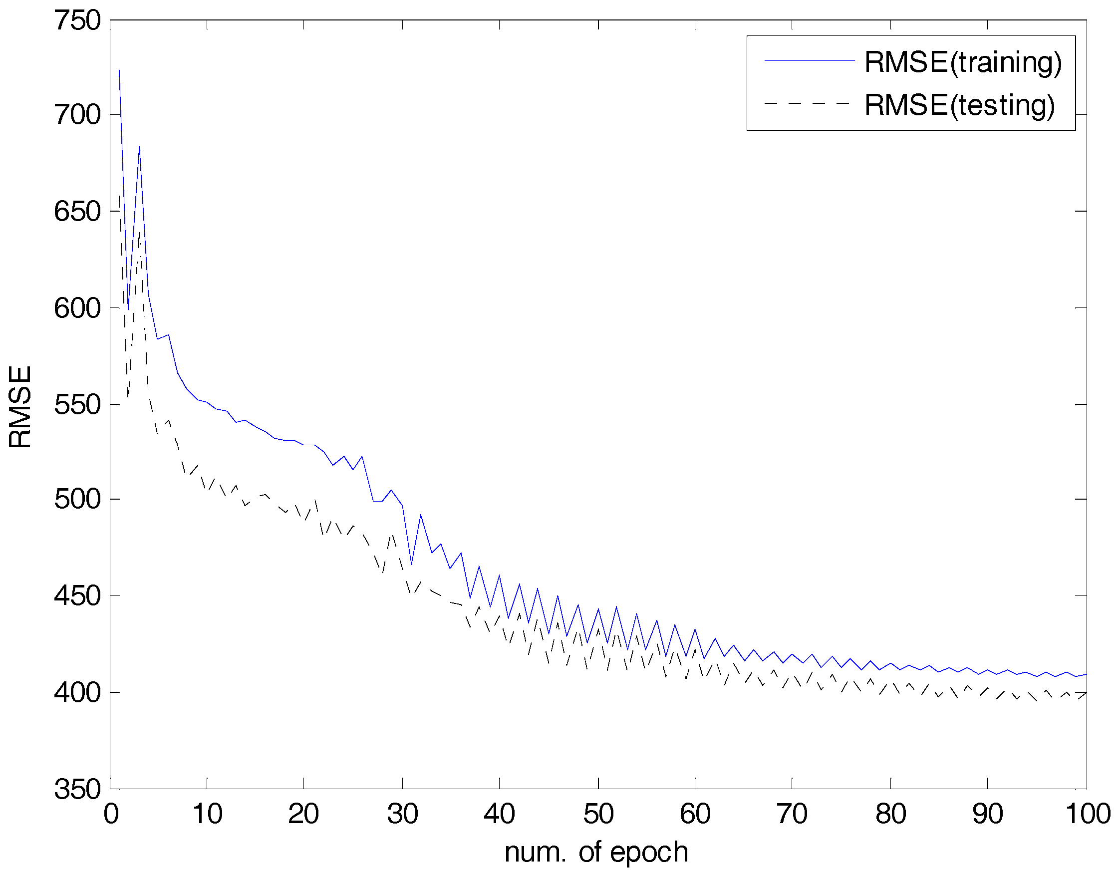
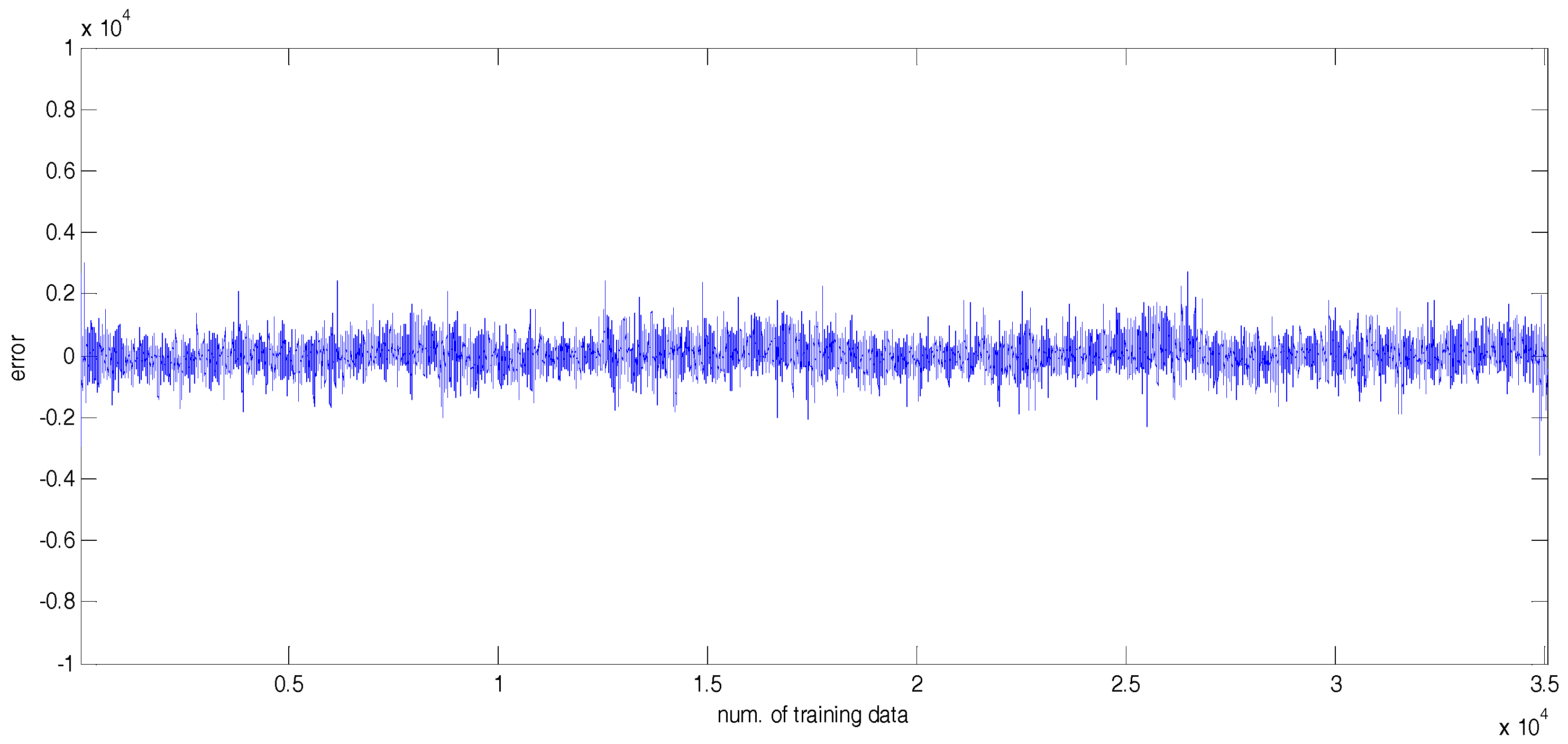
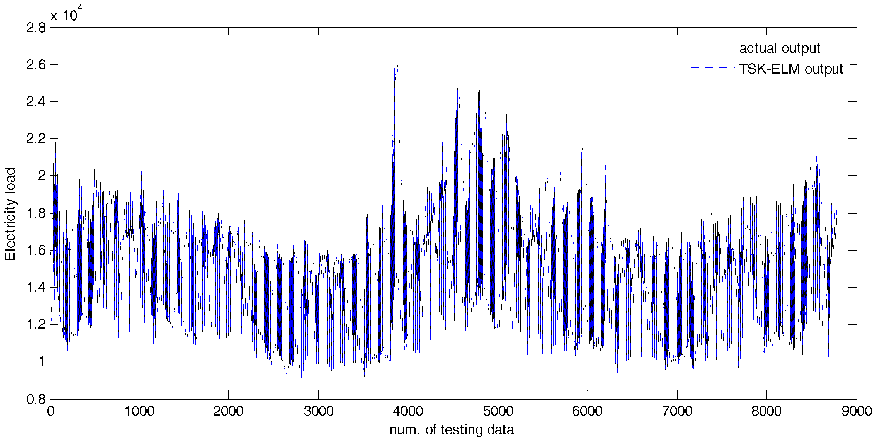
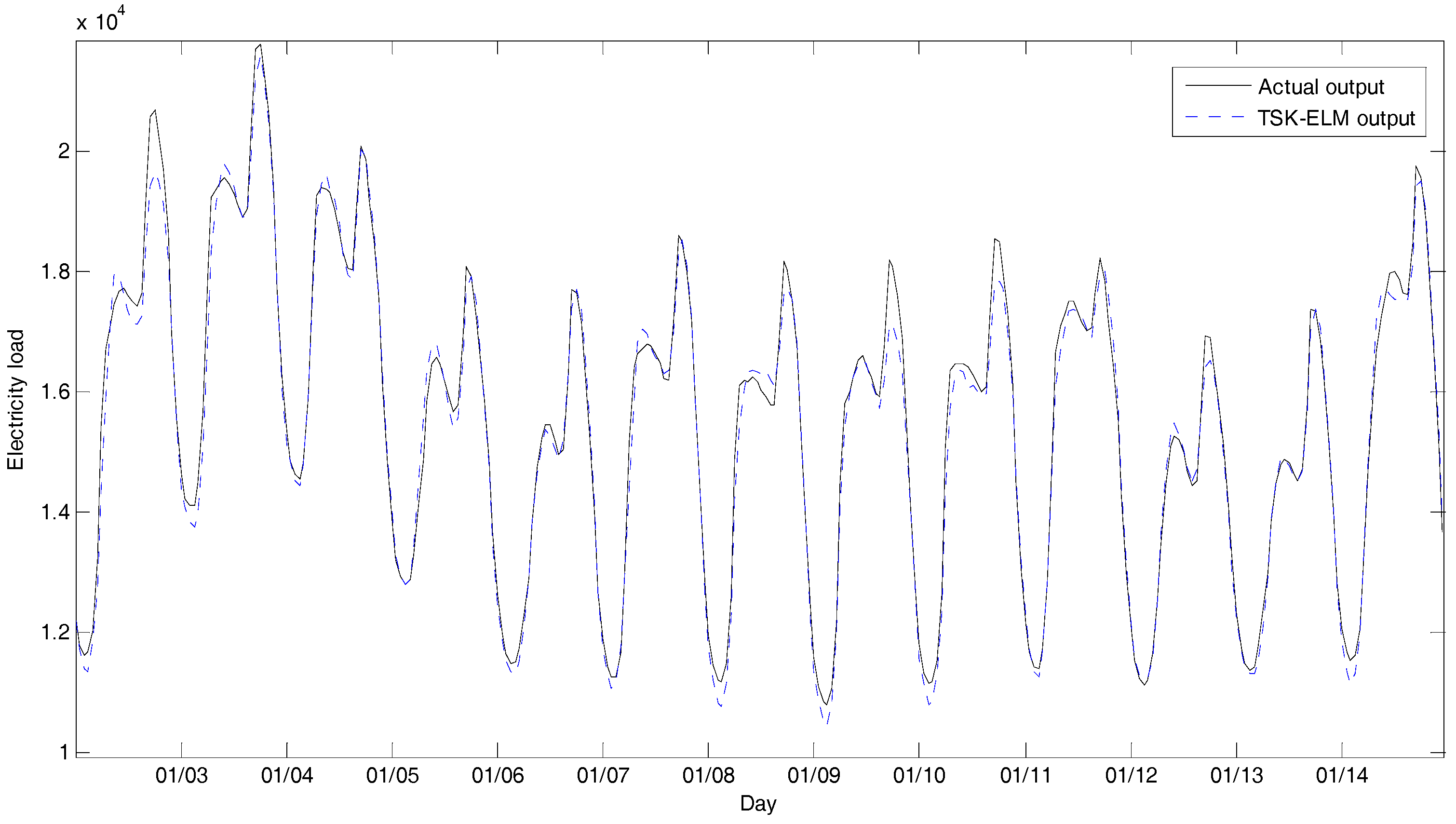
4.2. Experiments and Results

In this experiment, we compared the proposed method with conventional methods. We quantify the performance of the forecaster using metrics such as RMSE as well as MAE and MAPE. Also, we investigate statistical characteristics based on the coefficient of determination (R-squared) as follows
RMSE = 1 n k = 1 n ( t k y ^ k ) 2
MAE = k = 1 n | t k y ^ k | n
MAPE = 1 n k = 1 n | t k y ^ k | t k
R 2 = 1 k = 1 n ( t k y ^ k ) 2 k = 1 n ( t ¯ y ^ k ) 2
where y ^ k , t k , and t ¯ are model output, actual target output, and the mean of the actual output, respectively. n is the number of measured data points.
First, we obtained the root-mean-square error (RMSE) variation, as the number of cluster centers increased from 2 to 40. Here the number of cluster is equal to that of TSK-based fuzzy rule. Also, the Gaussian membership function per input variable is equal to that of cluster center. Figure 8 shows the RMSE values for the training and testing data sets. We observe that the RMSE value diminishes as the number of rules increases. The obtained results showed good generalization performance for testing data set, when the number of rules is 36. The RMSE of the testing error is at its lowest value: 400.86. Simultaneously, the RMSE of the training error is 402.89. Figure 9 shows the RMSE variation, when hybrid-learning is performed with five rules. The experimental results show a performance similar to the best case shown in Figure 8.
Figure 10 shows the prediction performance for all training data points. Figure 11 shows the TSK-ELM error for the training data points. As shown in Figure 10 and Figure 11, the proposed TSK-ELM shows a good approximation capability.
Figure 12 and Figure 13 visualize the generalization performance and error between the actual output and the TSK-ELM output for the testing data points. Figure 14 shows the performance for some period (some part of January in 2008) in the data set. As shown in these figures, the proposed method had a good generalization performance.
Table 1 lists the performance results of the RMSE regarding the previous model and the proposed approach. In the linguistic model (LM) design, we used 10 contexts and 10 clusters per context [29]. Thus, the number of rules was 100. This model lacked the adaptability to cover complex nonlinearity. In the RBFN design with context-based fuzzy c-means (CFCM) clustering, we used the number of clusters and the context in the same manner as the LM [30]. Here, the learning rate and the number of epochs are 0.001 and 1000, respectively. In the incremental RBFN design (IRBFN), we combined linear regression (LR) and RBFN [31]. LR and RBFN are used as the global model and local granular network, respectively. The error obtained from the LR is compensated by the local RBFN based on CFCM clustering. Here, the weights between the hidden layer and the output layer are estimated by LSE. Figure 15 shows the linguistic contexts produced from errors, when the number of contexts is 10. These contexts are obtained in error space based on CFCM clustering [30,31]. The errors obtained by LR are compensated by a collection of radial basis functions that capture more localized nonlinearities of the system as a local RBFN [31]. These contexts are used as the linguistic weights in the design of RBFN. In order to generate these contexts, we used fuzzy equalization and probabilistic distribution. Here, we use probabilistic distribution by histogram, probability density function, and conditional density function in order [31,32].
On the other hand, we performed on TSK-ELM based on scatter partition methods such as fuzzy c-means (FCM) clustering and subtractive clustering (SC). In the case of FCM clustering, we used 36 cluster centers as the number of rules. The experimental results of RMSE are 468.79 and 450.60 as listed in Table 1, respectively. In the case of SC clustering, we used 36 cluster centers as in the same manner. The experimental results of RMSE are 487.38 and 479.79, respectively. As a result, the proposed TSK-ELM showed good performance in comparison with those of scatter partition methods. Thus, the initial random-partition method of ELM used in this experiment demonstrated the effectiveness as the previous works [27].
In the ELM case, we used the ReLU, sigmoid, RBF, and sine functions as activation functions. Figure 16 visualizes the RMSE for the training and testing data sets as the number of nodes increases from 10 to 300. We observed that the ELM with the sine, sigmoid, and radial basis function showed similar performance except for ReLU activation function. However, we could not obtain the knowledge information about the ELM structure. Although these models have been successfully demonstrated on various applications, the proposed TSK-ELM outperformed the previous models as listed in Table 1.
In what follows, we quantified the performance between TSK-ELM and the previous methods using metrics such as of MAE and MAPE. To obtain further insight into the TSK-ELM performance for forecasting, we visualized the percent forecast errors by the hour of the day, day of the week, and month of the year as shown in Figure 17, respectively. On each box, the central mark indicates the median, and the bottom and top edges of the box indicate the 25% and 75% for MAPE, respectively. The whiskers extend to the most extreme data points not considered outliers, and the outliers are plotted individually using the “+” symbol.
Figure 18 shows performance results of MAPE by the number of node in the design of ELM with four activation functions, respectively. The experiment was performed as the number of node increase from 10 to 300. Figure 19 visualizes the distribution of error, MAE, and MAPE, respectively. Table 2 and Table 3 list the comparison results of MAPE and MAE, respectively. As listed in Table 2 and Table 3, these results led us to the conclusion that the proposed TSK-ELM without learning or with learning showed good performance in comparison to the previous methods such as ELM with four activation functions [21] and ANFIS with grid partition and input selection method [35]. We compared ELM (sin) with TSK-ELM based on the coefficient of determination (R-squared) showing statistical characteristics. R-squared values are 0.9783 and 0.9905 for ELM and TSK-ELM, respectively. These results provide a measure of how well the actual output is predicted by TSK-ELM model. In addition to R-squared values, the MAPE values of ELM are 2.16 and 2.14 for training and testing data, while those of TSK-LEM are 1.38 and 1.49 as listed in Table 3, respectively. As a result, the proposed TSK-ELM showed good performance in comparison to ELM itself.

5. Conclusions

We proposed a new design method based on an ELM with automatic knowledge representation from the numerical data sets for short-term electricity-load forecasting. The conventional ELM did not use knowledge information. The notable features of the proposed TSK-LEM were that the cluster centers of the membership function were used to determine the premise parameters, and the linear weights of the TSK-type were estimated by LSE.
The experimental results revealed that the proposed TSK-ELM showed good performance for short-term electricity-load forecasting in comparison to previous approaches such as LR, CFCM-RBFN, LM, IRBFN, and ELM with four activation functions. Furthermore, when a hybrid-learning method using LSE and BP was applied, the proposed model showed better prediction performance and statistical characteristics for RBSE, MAPE, MAE, and R-squared. For further research, we shall design an intelligent predictor by integrating an ELM with deep learning to solve real-world problems.

Acknowledgments

This research was supported by the “Human Resources Program in Energy Technology” of the Korea Institute of Energy Technology Evaluation and Planning (KETEP). Financial resources were granted by the Ministry of Trade, Industry and Energy, Republic of Korea (No. 20174030201620).

Author Contributions

Chan-Uk Yeom suggested the idea of the work and performed the experiments; Keun-Chang Kwak designed the experimental method; both authors wrote and critically revised the paper.

Conflicts of Interest

The authors declare no conflict of interest.

References

  1. Kyriakides, E.; Polycarpou, M. Short Term Electric Load Forecasting: A Tutorial. In Studies in Computational Intelligence; Springer: Berlin/Heidelberg, Germany, 2007; pp. 391–418. [Google Scholar]
  2. Zhang, Y.; Yang, R.; Zhang, K.; Jiang, H.; Jason, J. Consumption behavior analytics-aided energy forecasting and dispatch. IEEE Intell. Syst. 2017, 32, 59–63. [Google Scholar] [CrossRef]
  3. Dong, Y.; Ma, X.; Ma, C.; Wang, J. Research and application of a hybrid forecasting model based on data decomposition for electrical load forecasting. Energies 2016, 9, 1050. [Google Scholar] [CrossRef]
  4. Huang, N.; Lu, G.; Xu, D. A permutation importance-based feature selection method for short-term electricity load forecasting using random forest. Energies 2016, 9, 767. [Google Scholar] [CrossRef]
  5. Bennett, C.; Stewart, R.A.; Lu, J. Autoregressive with exogenous variables and neural network short-term load forecast models for residential low voltage distribution networks. Energies 2014, 7, 2938–2960. [Google Scholar] [CrossRef]
  6. Hernandez, L.; Baladron, C.; Aguiar, J.M.; Carro, B.; Sanchez-Esguevillas, A.J.; Lloret, J. Short-term load forecasting for microgrids based on artificial neural networks. Energies 2013, 6, 1385–1408. [Google Scholar] [CrossRef]
  7. Amjady, N.; Keynia, F. A new neural network approach to short term load forecasting of electrical power systems. Energies 2011, 4, 488–503. [Google Scholar] [CrossRef]
  8. Goude, Y.; Nedellec, R.; Kong, N. Local short and middle term electricity load forecasting with semi-parametric additive models. IEEE Trans. Smart Grid 2014, 5, 440–446. [Google Scholar] [CrossRef]
  9. Guo, H. Accelerated continuous conditional random fields for load forecasting. IEEE Trans. Knowl. Data Eng. 2015, 27, 2023–2033. [Google Scholar] [CrossRef]
  10. Yu, C.N.; Mirowski, P.; Ho, T.K. A sparse coding approach to household electricity demand forecasting in smart grids. IEEE Trans. Smart Grid 2017, 8, 738–748. [Google Scholar] [CrossRef]
  11. Chen, Y.; Xu, P.; Chu, Y.; Li, W.; Wu, Y.; Ni, L.; Bao, Y.; Wang, K. Short-term electrical load forecasting using the support vector regression model to calculate the demand response baseline for office buildings. Appl. Energy 2017, 195, 659–670. [Google Scholar] [CrossRef]
  12. Ren, Y.; Suganthan, P.N.; Amaratunga, G. Random vector functional link network for short-term electricity load demand forecasting. Inf. Sci. 2016, 367–368, 1078–1093. [Google Scholar] [CrossRef]
  13. Lopez, C.; Zhong, W.; Zheng, M. Short-term electric load forecasting based on wavelet neural network, particle swarm optimization and ensemble empirical mode decomposition. Energy Procedia 2017, 105, 3677–3682. [Google Scholar] [CrossRef]
  14. Zhang, R.; Dong, Z.Y.; Xu, Y.; Meng, K.; Wong, K.P. Short-term load forecasting of Australian national electricity market by an ensemble model of extreme learning machine. IET Gener. Transm. Distrib. 2013, 7, 391–397. [Google Scholar] [CrossRef]
  15. Golestaneh, F.; Pinson, P.; Gooi, H.B. Very short-term nonparametric probabilistic forecasting of renewable energy generation-with application to solar energy. IEEE Trans. Power Syst. 2016, 31, 3850–3863. [Google Scholar] [CrossRef]
  16. Li, S.; Wang, P.; Goel, L. A novel wavelet-based ensemble method for short-term load forecasting with hybrid neural networks and feature selection. IEEE Trans. Power Syst. 2016, 31, 1788–1798. [Google Scholar] [CrossRef]
  17. Cecati, C.; Kolbusz, J.; Rozycki, P.; Siano, P.; Wilamowski, B.M. A novel RBF training algorithm for short-term electric load forecasting and comparative studies. IEEE Trans. Ind. Electron. 2015, 62, 6519–6529. [Google Scholar] [CrossRef]
  18. Li, S.; Wang, P.; Goel, L. Short-term load forecasting by wavelet transform and evolutionary extreme learning machine. Electr. Power Syst. Res. 2015, 122, 96–103. [Google Scholar] [CrossRef]
  19. Yang, Z.; Ce, L.; Lian, L. Electricity price forecasting by a hybrid model, combining wavelet transform, ARMA and kernel-based extreme learning machine methods. Appl. Energy 2017, 190, 291–305. [Google Scholar] [CrossRef]
  20. Li, S.; Goel, L.; Wang, P. An ensemble approach for short-term load forecasting by ELM. Appl. Energy 2016, 170, 22–29. [Google Scholar] [CrossRef]
  21. Huang, G.B.; Zhou, H.; Ding, X.; Zhang, R. Extreme learning machine for regression and multiclass classification. IEEE Trans. Syst. Man Cybern. Part B 2012, 42, 513–529. [Google Scholar] [CrossRef] [PubMed]
  22. ISO. New England. Available online: https://en.wikipedia.org/wiki/ISO_New_England (accessed on 13 October 2017).
  23. Mathworks. Available online: https://www.mathworks.com/videos/electricity-load-and-price-forecasting-with-matlab-81765.html (accessed on 13 October 2017).
  24. Zhang, R.; Lan, Y.; Huang, G.B.; Xu, Z.B. Universal approximation of extreme learning machine with adaptive growth of hidden nodes. IEEE Trans. Neural Netw. Learn. Syst. 2012, 23, 365–371. [Google Scholar] [CrossRef] [PubMed]
  25. Huang, G.B.; Bai, Z.; Kasun, L.L.C.; Vong, C.M. Local receptive fields based extreme learning machine. IEEE Comput. Intell. Mag. 2015, 10, 18–29. [Google Scholar] [CrossRef]
  26. Neumann, K.; Steil, J.J. Optimizing extreme learning machines via ridge regression and batch intrinsic plasticity. Neurocomputing 2013, 102, 23–30. [Google Scholar] [CrossRef]
  27. Deng, Z.; Choi, K.S.; Cao, L.; Wang, S. T2FELA: Type-2 fuzzy extreme learning algorithm for fast training of interval type-2 TSK fuzzy logic system. IEEE Trans. Neural Netw. Learn. Syst. 2014, 25, 664–676. [Google Scholar] [CrossRef] [PubMed]
  28. Jang, J.S.R.; Sun, C.T.; Mizutani, E. Neuro-Fuzzy and Soft Computing: A Computational Approach to Learning and Machine Intelligence; Prentice Hall: Upper Saddle River, NJ, USA, 1997. [Google Scholar]
  29. Han, Y.H.; Kwak, K.C. A design of an improved linguistic model based on information granules. J. Inst. Electron. Inf. Eng. 2010, 47, 76–82. [Google Scholar]
  30. Pedrycz, W. Conditional fuzzy clustering in the design of radial basis function neural networks. IEEE Trans. Neural Netw. 1998, 9, 601–612. [Google Scholar] [CrossRef] [PubMed]
  31. Lee, M.W.; Kwak, K.C. A design of incremental granular networks for human-centric system and computing. J. Korean Inst. Inf. Technol. 2012, 10, 137–142. [Google Scholar]
  32. Kwak, K.C.; Kim, S.S. Development of quantum-based adaptive neuro-fuzzy networks. IEEE Trans. Syst. Man. Cybern. Part B 2010, 40, 91–100. [Google Scholar]
  33. Box, G.E.P.; Jenkins, G.M.; Reinsel, G.C. Time Series Analysis: Forecasting and Control, 4th ed.; John Wiley & Sons: Hoboken, NJ, USA, 2008. [Google Scholar]
  34. Han, J.S.; Kwak, K.C. Image classification using convolutional neural network and extreme learning machine classifier based on ReLU function. J. Korean Inst. Inf. Technol. 2017, 15, 15–23. [Google Scholar]
  35. Pal, S.; Sharma, A.K. Short-term load forecasting using adaptive neuro-fuzzy inference system. Int. J. Novel Res Electr. Mech. Eng. 2015, 2, 65–71. [Google Scholar]
Figure 1. Architecture of a conventional ELM predictor.
Energies 10 01613 g001
Figure 2. Architecture of TSK-ELM with knowledge information.
Energies 10 01613 g002
Figure 3. Simplified architecture of TSK-ELM.
Energies 10 01613 g003
Figure 4. Diagram of the hybrid-learning procedure.
Energies 10 01613 g004
Figure 5. Input variables and output variable.
Energies 10 01613 g005
Figure 6. Data distribution between input variables (a) dew point and dry bulb temperature and (b) average load of the previous day and the load from the same hour the previous day
Energies 10 01613 g006
Figure 7. Histogram of actual output.
Energies 10 01613 g007
Figure 8. RMSE by rule number variation (TSK-ELM).
Energies 10 01613 g008
Figure 9. RMSE by hybrid learning (num. of rules = 5).
Energies 10 01613 g009
Figure 10. Prediction performance for training data points.
Energies 10 01613 g010
Figure 11. TSK-ELM error for training data points.
Energies 10 01613 g011
Figure 12. Prediction performance for testing data points.
Energies 10 01613 g012
Figure 13. TSK-ELM error for testing data points.
Energies 10 01613 g013
Figure 14. Performance for some period of testing data sets.
Energies 10 01613 g014
Figure 15. Linguistic contexts obtained by IRBFN.
Energies 10 01613 g015
Figure 16. Performance results of the conventional ELM. (a) ReLU; (b) sigmoid; (c) RBF; and (d) sine.
Energies 10 01613 g016
Figure 17. RMSE divided by each output point. (a) hour of day; (b) day of week; (c) month of year.
Energies 10 01613 g017
Figure 18. Performance results of MAPE by the number of node (ELM with four activation functions). (a) ReLU; (b) sigmoid; (c) RBF; and (d) sine.
Energies 10 01613 g018
Figure 19. Distribution of (a) error; (b) MAE; and (c) MAPE.
Energies 10 01613 g019
Table 1. Comparison results of RMSE (*: no. of rule).
MethodNo. of NodeRMSE (Training)RMSE (Testing)
LR [33]-1044.5928.98
RBFN(CFCM) [30]100983.64926.43
LM [29]100 *1005.61980.59
IRBFN [31]450647.10450.60
ELM (ReLU) [34]260620.35586.11
ELM (Sigmoid) [21]270451.56438.52
ELM (RBF) [21]300449.88433.99
ELM (sin) [21]270443.16435.07
TSK-ELM (FCM)36 *468.79450.60
TSK-ELM(SC)36 *487.38478.79
TSK-ELM (without learning)36 *402. 89400.86
TSK-ELM (with learning)5 *409.31398.58
10 *359.24349.61
36 *292.93331.16
Table 2. Comparison results of MAPE (*: no. of rule).
MethodNo. of NodeMAPE(%)-TrainingMAPE(%)-Testing
ELM (ReLU) [34]3002.942.87
ELM (Sig) [21]2902.182.15
ELM (RBF) [21]3002.232.19
ELM (sin) [21]3002.162.14
ANFIS [35]36 *3.323.27
TSK-ELM (without learning)36 *2.011.99
TSK-ELM (with learning)5 *1.961.95
10 *1.721.70
36 *1.381.49
Table 3. Comparison results of MAE (*: no. of rule).
MethodNo. of NodeMAE(MWh)-TrainingMAE (MWh)-Testing
ELM (ReLU) [34]300445.54427.08
ELM (Sig) [21]290331.06320.69
ELM (RBF) [21]300338.91326.21
ELM (sin) [21]300328.71319.18
ANFIS [35]36 *500.84483.11
TSK-ELM (without learning)36 *306.62298.21
TSK-ELM (with learning)5 *300.53292.14
10 *264.65257.19
36 *213.72227.48

