Community Microgrid Scheduling Considering Network Operational Constraints and Building Thermal Dynamics †


1
Power & Energy Systems Group, Oak Ridge National Laboratory, Oak Ridge, TN 37831, USA
2
Department of Electrical Engineering and Computer Science, The University of Tennessee, Knoxville, TN 37996, USA
*
Author to whom correspondence should be addressed.
†
This manuscript has been authored by UT-Battelle, LLC under Contract No. DE-AC05-00OR22725 with the U.S. Department of Energy. The United States Government retains and the publisher, by accepting the article for publication, acknowledges that the United States Government retains a non-exclusive, paid-up, irrevocable, world-wide license to publish or reproduce the published form of this manuscript, or allow others to do so, for United States Government purposes. The Department of Energy will provide public access to these results of federally sponsored research in accordance with the DOE Public Access Plan (http://energy.gov/downloads/doe-public-access-plan).
Energies 2017, 10(10), 1554; https://doi.org/10.3390/en10101554
Submission received: 16 August 2017
/
Revised: 19 September 2017
/
Accepted: 27 September 2017
/
Published: 10 October 2017
(This article belongs to the Section F: Electrical Engineering)
Abstract
:This paper proposes a Mixed Integer Conic Programming (MICP) model for community microgrids considering the network operational constraints and building thermal dynamics. The proposed multi-objective optimization model optimizes not only the operating cost, including fuel cost, electricity purchasing/selling, storage degradation, voluntary load shedding and the cost associated with customer discomfort as a result of the room temperature deviation from the customer setting point, but also several performance indices, including voltage deviation, network power loss and power factor at the Point of Common Coupling (PCC). In particular, we integrate the detailed thermal dynamic model of buildings into the distribution optimal power flow (D-OPF) model for the optimal operation. Thus, the proposed model can directly schedule the heating, ventilation and air-conditioning (HVAC) systems of buildings intelligently so as to to reduce the electricity cost without compromising the comfort of customers. Results of numerical simulation validate the effectiveness of the proposed model and significant savings in electricity cost with network operational constraints satisfied.
1. Introduction
A microgrid is a small-scale and low voltage power system comprising various distributed generation facilities, such as distributed generators (DG) and energy storage. A microgrid has two operating modes: grid-connected and islanded [1]. It is connected to the main grid with a single point interface, the Point of Common Coupling (PCC). Through PCC, a microgrid can not only purchase electricity from or sell electricity back to the main grid, but also provide other services, such as voltage and frequency regulation [2,3]. By coordinating DG, energy storage and demand response, a microgrid can improve the reliability of local electricity supply with lower cost and emissions [4]. Therefore, research on microgrid has been growing recently [5].
The scheduling of microgrids in either grid-connected or islanded modes is usually performed by a microgrid controller. It optimizes the dispatch of controllable DG and the power exchanging at PCC with the main grid by solving a economic dispatch or unit commitment problem. The optimization is subject to various environmental, reliability and operating constraints. There has been extensive research on the scheduling of microgrids [6]. Various models are proposed for microgrid scheduling in islanded model [7,8,9,10] and grid-connected mode [11,12,13,14,15]. In particular, Sobu et al. [11,12] proposed deterministic models, while Cardoso et al. [13,14] proposed stochastic models considering uncertainty of renewable generation. Liu et al. [15] designed a hybrid stochastic/robust programming model. However, in most of existing literature, network configuration, reactive power flow and power factor constraints have been mostly ignored in the optimization model. Under this assumption, the voltage and power factor limits as well as line thermal limits may not be satisfied by the solution. For this reason, economic and secure operation of microgrids requires solving the distribution optimal power flow (D-OPF) considering the distribution network, voltage and power factor limits, and so on. The D-OPF problem has been researched extensively and various methods has been proposed. Gradient search and interior point methods are directly used to solve the nonlinear and non-convex D-OPF problem in [16,17,18]. However, solving non-convex programming is very time consuming, while the real-time control of microgrids normally has strict time requirements. Besides, the global optimum cannot be guaranteed. For this reason, Borghetti et al. [19,20,21,22,23] proposed sensitivity based linear programming model for the D-OPF problem. The distribution network is directly linearized at current operating point by calculating the sensitivity coefficients. Nevertheless, the sensitivity coefficients need to be updated continuously, which is still time consuming. More popularly, the non-linear/non-convex items in the D-OPF problem are directly approximated or relaxed into linear/convex form. In particular, the D-OPF is approximated as linear programming [24,25]; or semidefinite programming (SDP) [26]; or second-order cone programming (SOCP) using either polar coordinates [27]. DistFlow model is proposed in [28,29]. The non-convex D-OPF is directly relaxed into convex conic programming. The solution efficiency can been improved significantly with accuracy preserved. For this reason, DistFlow model has been widely used in various research recently.
In the existing literature, HVAC consumption is mostly considered as a responsive load, which could be postponed, or as a simple non-controllable load. The thermal dynamic characteristics of buildings as well as the customer comfort preference are seldom taken into account. In fact, the slow thermal dynamic characteristic of buildings make HVAC systems perfect candidates for demand side management due to building thermal inertia. With a range of allowable indoor temperature (desired temperature with allowed temperature deviation) set by consumers/building owners, our goal is to shift the consumption of HVAC during peak price time to low price time as much as possible while keeping the indoor temperature inside the limits. Since the indoor temperature changes very slow due to the thermal inertia, the buildings/houses can be pre-cooled (or pre-heated) during low price time, then ride through the peak price time without or with less consumption. Thus, the electricity cost of customers can be reduced significantly without compromising their comfort. To realize this benefit, the microgrid scheduling model has to include the thermal dynamic characteristics of buildings/houses as constraints and directly determine the on/off of HVAC systems together with the dispatch of DG and energy storage. The home energy management system considering thermal dynamic model of houses has been proposed in in [14,30] in recent years. However, it was model as a continuous variable. In fact, most existing HVAC systems in houses have only two states, on and off. Besides, the network configuration, voltage and power factor limits are neglected.
In this paper, we propose a new mixed integer conic programming (MICP) model for community microgrids considering the network operational constraints and building thermal dynamics. The proposed optimization framework optimizes both operating cost and system performance. Voltage deviation, network power loss and power factor at PCC are the performance indices considered in the model. Detailed thermal dynamic characteristics of buildings are integrated into the proposed community microgrid scheduling model. The main contributions of this paper are as follows:
- A multi-objective optimization model is proposed to optimize both the operating cost and performance indices of a microgrid. The analytical hierarchy process (AHP) has been introduce to calculate the weighting coefficients of different objectives [31].
- The building thermal dynamics and HVAC controllers have been integrated into the microgrid scheduling model. The HVAC systems are directly scheduled by the microgrid controller and the operating cost are reduced significantly; and
- The proposed model has been validated in various simulation cases.
The rest of this paper is organised as follows: The community microgrid is introduced in Section 2. The thermal dynamic model of houses are proposed and linearized. Based on those models, we proposed the optimization model for community microgrid scheduling considering network operational constraints and building thermal dynamics is proposed in Section 3. Results of numerical simulation of various cases and sensitivity analysis are presented in Section 4. At last, we draw conclusions in Section 5.
2. System Modeling
2.1. Community Microgrid Model
A community microgrid is a special kind of microgrid serving residential communities. The load of a community microgrid are normally a number of houses. It is connected to the main utility distribution network through PCC, but can also isolate from the utility distribution network and serve customers by various onsite DG and energy storage. In each house, there might be rooftop PV panels, small batteries and EVs existing. A building energy management system (BEMS) controls all appliances in each house and communicate with the community microgrid controller. In general, the community microgrid controller coordinates the dispatch of DG and energy storage, consumption of customers and power exchanging at PCC to minimize the operating cost of the community microgrid subject to operational and technical constraints. Particularly, all BEMSs forward the indoor temperature settings, house thermal parameters and other load information to the community microgrid controller. Then, the microgrid controller will solve the proposed optimization and send the schedule of HVAC system as well other controllable appliances to each BEMS. The BEMS will control the HVAC and other controllable appliance accordingly. An example of the community microgrid under consideration is shown in Figure 1.
2.2. HVAC System Model
Typically, the HVAC system inside a house is controlled by a thermostats, which includes a temperature sensor and a temperature controlled relay circuit. As a rule, the desired indoor temperature and allowed temperature deviation are preset by customers according to their personal preferences. Based on the indoor temperature measured by the temperature sensor, the temperature relay will determine the on and off status of HVAC. Take cooling for example, the HVAC will be turned on whenever the indoor temperature violates the up limit of allowed temperature. It continues running until the indoor temperature is lower than the lower limit of the allowed indoor temperature. Due to the lower cost of thermostats, this automatic temperature control scheme has been widely used in practice.
In this paper, we assume the BEMS inside each house will forward the temperature settings of customers to the community microgrid controller. Thus, the community microgrid controller can coordinate the consumption of customer with DG and renewable energy generation as well as electricity price at PCC, so as to schedule the HVAC and other controllable house appliances intelligently. Due to the thermal inertia of buildings/houses, the buildings/houses can be pre-cooled (or pre-heated) during low price time, then ride through the peak price time without or with less consumption while still keeping the indoor temperature inside the limits. As a result, we expected significant savings in electricity cost comparing with the automatic temperature control above.
2.3. Building Thermal Dynamic Model
In this paper, a two-layer thermal insulation model is used for the thermal modeling of buildings/houses. Based on the rules of heat transfer, a third order linear model is established for the thermal dynamic analysis of a building/house [32]. The model is represented as differential Equations (1)–(3) as:
The equivalent thermal parameters and are assumed to be constant for a house h, which can be estimated by using various methods based on measured data [33,34]. Thus, the above thermal dynamics of house h can be rewritten in the linear state-space model in continuous time as:
where is the state vector. is the input vector. The coefficients of matrices and of a house h can be calculated based on the effective window area, the fraction of solar irradiation entering the inner walls and floor, the thermal capacitance and resistance parameters of the house. The state-space model in continuous time Equation (4) can be further transformed into equivalent discrete time model Equation (5) by using Euler discretization (i.e., zero-order hold) with a sampling time [32,35].
where and are constant, which can be calculated based on , and the sampling time. Note that the discrete time model will be used in the rest of this paper. Please refer to [32] for more detailed information on the thermal dynamic modeling of buildings/houses. The indoor temperature of a building/house is constrained by Equation (6) as following:
3. Problem Formulation
3.1. Objective
For the community microgrids under consideration in this paper, all loads are served by local distributed resources and the main distribution utility through PCC. The distributed resources are divided into two categories: dispatchable and non-dispatchable units. The real and reactive power out put of dispatchable units can be controlled by the community microgrid controller subject to various technical and operating constraints. In contrast, non-dispatchable units, such as PV panels are not controllable since their output are closed related with the weather conditions, which is difficult to be predicted. The power exchanging at PCC between the microgrid and distribution utility is conducted under a forecast day-ahead market price for a time window of 24 h. Each house or building is associated with a HVAC load and a non-HVAC load. Under these assumptions, the objective of the proposed microgrid controller aims at minimizing a virtual cost associated with the operating cost and performance of a micorgrid as in Equation (7). In specific, the first line is the linearized fuel cost of DGs and the second line is the start-up cost; the third line is the discomfort cost of customers due to the deviations between actual temperature and customer desired temperature and cost of load shedding; the fourth line is the power exchanging cost/benefit at PCC and the energy storage degradation cost; the voltage deviation is calculated in line fifth and sixth; and the seventh line is the network power loss and the total absolute value of reactive power exchanging at PCC. All objectives are summed into a single objective function with corresponding weighings.
In this paper, the analytical hierarchy process (AHP) is used to determine the weighting coefficients , , and [31]. By AHP, the system operators can calculate the weighting coefficients of all objectives based on the pairwise comparison of relative importance of any two objectives. More details on how to calculate the weighting coefficients by AHP will be introduced in Section 4.
3.2. Constraints
For the secure and economic operation of the community microgrid, A number of technical constraints associated with DGs, energy storage, HVAC systems, house appliances and distribution network should be satisfied. These constraints are presented in this section.
3.2.1. Constraints of DGs
Normally, DGs are subject to the following constraints:
3.2.2. Constraints of Energy Sotrage
The energy storage is operated subject to the following constraints:
First of all, the maximum charging/discharging power of a energy storage is limited by constraint Equations (13) and (14). An energy storage can only be either charging or discharging at any moment, which is ensured by Equation (15). The state of charge (SOC) limits are represented by Equations (16) and (17). In Equation (16), the battery SOC at the end of current time interval equals to the SOC at the end of last time interval plus the energy charged minus the energy discharged during current interval. The charging and discharging of battery is subject to loss, which is represented by parameter and . The energy storage outputs are subject to power factor limits in both charging and discharging states as in Equations (18) and (19). Constraints Equations (18) and (19) are reformulated into mixed integer linear (MIL) format in Section 3.3. The power capacity limit of inverters associated with the energy storage is guaranteed by Equations (20) and (21).
3.2.3. Load Constraints
For each house, the load is divided into HVAC load and non-HVAC load as in Equations (22) and (23). The constraints associated with HVAC systems include Equations (5) and (6). A HVAC system can only be operated at either heating or cooling modes at any moment, which is enforced by Equation (24). The amount of load curtailment in house h during time interval t is limited by constraint Equations (25) and (26).
3.2.4. Network Constraints
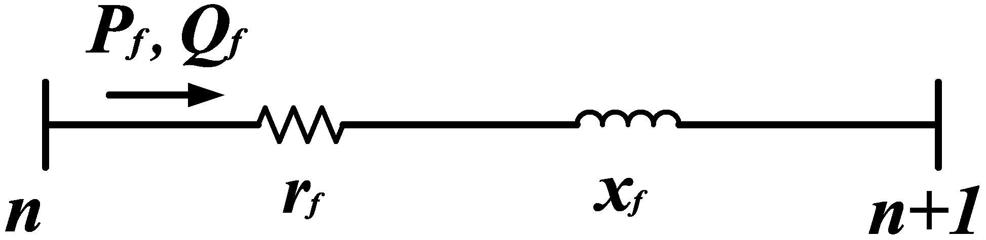
The model of a distribution feeder with bus n as sending end and bus as receiving end is shown in Figure 2. Considering the power flow direction as depicted in Figure 2. Equations (27)–(30) represents the DistFlow equations, which have been validated in [26,29]. Equation (27) represents the voltage drop between two adjacent buses along a feeder. The real and reactive power balance for each node are guaranteed by Equations (28) and (29), where and are the incidence matrix for the sending end line flow and line losses. is 1 if bus n is the sending end of line f, and −1 if bus n is the receiving end of line f and zero if neither terminal of line f is connected to bus n. is 1 if bus n is the receiving end of line f and zero for all other elements. It should be noted that and should be included in Equations (28) and (29) for the PCC node. The quadratic equality constraint in Equation (30) is nonconvex, but we can relax Equation (30) into convex inequalities as in Equation (31) by conic relaxation. For the accuracy of the conic relaxation in optimal power flow (OPF) problem, we refer readers to [36,37], which compare the conic relaxation based OPF results with standard nonlinear programming (NLP) based OPF results for different IEEE test systems. Equation (32) is a standard second order cone formulation of Equation (31). Note that only Equation (32) will be used in the problem formulation instead of Equations (30) and (31). The maximum bus voltage deviation is limited by Equations (33) and the thermal limits of distribution feeders are enforced by Equation (34). it should be noted that the square of nodal voltages in Equations (27) and (33) are directly taken as variables. Hence, Equations (27) and (33) are linear.
3.2.5. Constraints at PCC
At the PCC, the exchanged power at PCC is subject to a maximum value due to line capacity or reliability requirements as in Equation (35). The power factor limit at PCC is ensured by Equation (36). In addition, the PCC voltage is normally determined by the utility network operating condition, which is specified in Equation (37).
3.3. Simplification and Linearization
At this moment, we have almost completed the formulation of the proposed D-OPF model for community microgrid scheduling. However, there are several logic or non-convex items in the objective and constraints. In this subsection, we will reformulate all logic or non-convex items into equivalent mixed integer linear (MIL) form, so that the proposed D-OPF problem is a MICP, which could be solved by commercial solvers efficiently. In the objective function, we could easily recast the startup cost of DGs (line 2) into MIL form by introducing another binary variable for each DG in every time interval as in [38]. As to the voltage deviation (line 5 and 6), we introduce auxiliary continuous variable , which represents the absolute value of voltage deviation. Constraints Equations (38)–(40) are equivalent MIL form of the absolute function. Similarly, the customer discomfort cost (line 3) can be recast into Equations (41)–(43) with auxiliary variable representing the absolute value of temperature deviation. The same technique can linearize other absolution functions in Equations (7) and (36) into MIL format.
The logical terms in battery constraints Equations (18) and (19) can be reformulated into MIL form, as Equations (44) and (45) by the reuse of binary charging/discharging indicators
Finally, the objective function has been reformulated into MIL form and all constraints are either MIL or second order cones (SOC). Thus, the proposed D-OPF problem is a MICP, which could be solved by commercial solvers efficiently.
4. Case Studies
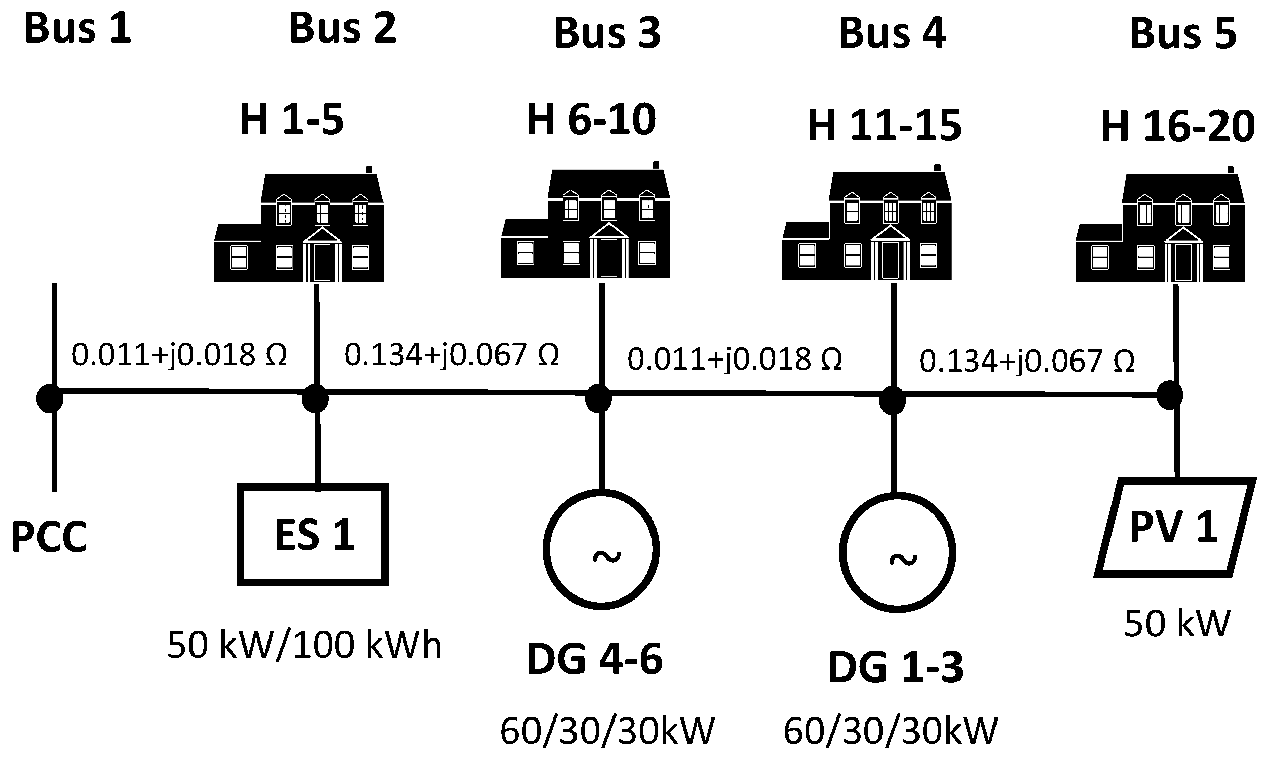
In this Section, we validate the proposed D-OPF model on a ORNL microgrid test system as shown in Figure 3. A number of DERs exist in the test system. Parameters for the dispatchable generators, PV, wind turbine and battery can be found in [15]. To guarantee operating in islanded mode without load shedding, we add another three dispatchable generators by duplicating the existing ones. For meteorological data, we use the measured 1 min solar irradiance and temperature of Oak Ridge, Tennessee area on 1 August 2015 from [39], which represents a typical summer day in the southeast of the US. In the system, there are 20 houses, equipped with a 5 kW HVAC system with a coefficient of performance (COP) for each house. The indoor temperature is set at 23 °C and the allowed deviation is ±2 °C. The customer discomfort factor is set at $0.05/°C. The thermal parameter of houses are from Table 7.1 in [32]. Random errors are generated and added to the parameters of each house to represent the variety of the houses. To be reasonable, the random errors are generated based on the standard deviation of the parameters’ estimation in [32] (again Table 7.1). The value of lost load (VOLL) is set as $2.0/kWh. The maximum load shedding is set as 10% of the non-HVAC load in each house. Since a variety of DGs and energy storage systems as well as various houses with different parameters have been considered in the microgrid test system, it should covers a wide variety of both existing and future community microgrids.
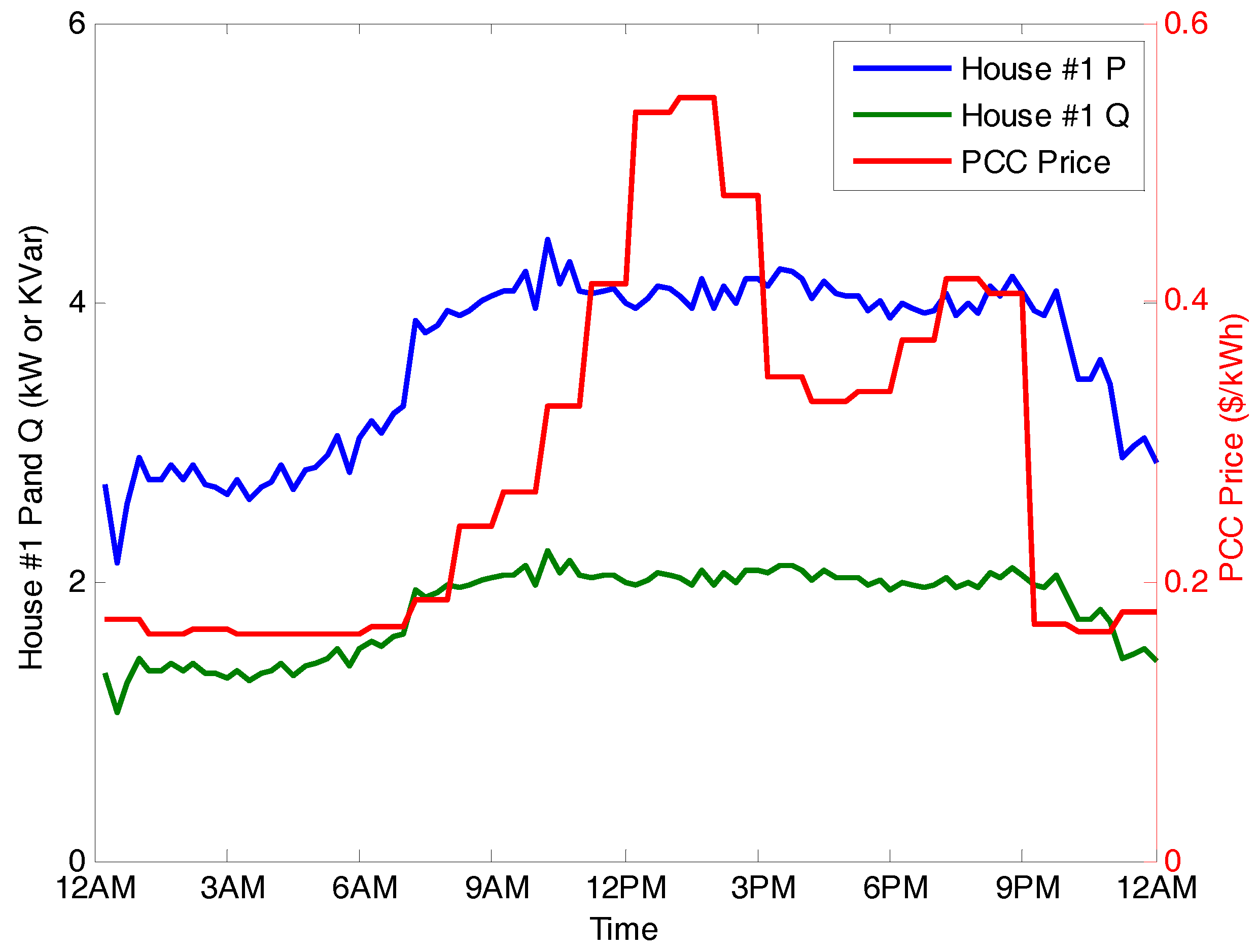
The optimization is running for a day (24 h horizon) with 15 min time intervals. The PV model is the same as in [18]. The forecast non-HVAC demand in house # 1 and the day-ahead market prices at the PCC are shown in Figure 4. The non-HVAC load curves of other houses are assumed the same. The power factor of HVAC is assumed 0.9 and the power factor at PCC is required to be no less than 0.9. All cases are solved using the MICP solver CPLEX 12.6. With a pre-specified duality gap of 0.5%, the average solution time is about 1 min on a 2.66 GHz Windows-based PC with 4 G bytes of RAM.
4.1. Effect of Weighting Factors
In this section, we will introduce how to calculate the weighting coefficients of multi-objectives by the AHP. For simplicity, fuel cost, purchasing cost, battery degradation cost, load shedding cost and customers’ discomfort cost are aggregated together as total cost with weighting coefficient . Generally, there are two steps. In the first step, a pairwise comparison of relative importance or priority between each two objectives is done. A pairwise comparison matrix can be established as in Table 1. For each position in the matrix, the importance of the objective at the left is compared with that of the objective at the top and the ratio is entered. In the second step, the AHP retrieves the weighting coefficients of all objectives by solving a trivial eigenvalue problem. If the pairwise comparison matrix is consistent, it is rank one and thus all its eigenvalues but one are equal to zero. This largest eigenvalue, i.e., principal eigenvalue is unique and equals to the dimension of the matrix. The corresponding eigenvector, i.e., principal eigenvector is positive and unique. The weighting coefficients of objectives can be obtained by normalizing this principal eigenvector of the pairwise comparison matrix. Since each element in the pairwise comparison matrix is directly estimated by comparing the priority of two corresponding objectives, the pairwise comparison matrix is very unlikely to be consistent, especially when the number of objective is large. According to [31], a consistency of about 10% is considered acceptable. In the inconsistent case, the principal eigenvalue is still unique and near the dimension of the matrix. The weighting coefficients of objectives can be obtained in the same way.
A typical pairwise comparison matrix is shown in Table 1, the corresponding weighting coefficients are calculated as: = 0.2084, = 0.1171, = 0.6116, and = 0.0629. It should be noted that the weighting coefficients are calculated based on the pairwise comparison matrix, which is established by system operators based on their own preference.
To compare the differences between single objective optimization and multi-objective optimization, we solve the single objective optimization problems for each objective. Then, we solve the multi-objective optimization problem using the calculated weighting coefficients above. We evaluate each solution by calculating all objective items, i.e., total cost, network loss, voltage deviation and total reactive power at PCC. The results are compared in Table 2.
For single objective optimization, the exclusive remaining objective is always optimized to be the best (as shown in red) compared to that of other solutions (the rest in the same row) by sacrificing other neglected objectives. While in multi-objective optimization, all objectives are considered and balanced by corresponding weighting coefficients. As a result, all objectives are optimized together, but none of them are as good as that of the corresponding single objective optimization. Nevertheless, all of these solutions are Pareto solutions, i.e., one cannot improve one term without sacrificing another.
4.2. Comparison of Cost between Different Control Methods
In this section, we compare the values of total objective and individual objectives calculated by the proposed optimization and that of autonomous temperature control. For autonomous control, we directly solve Equation (5) and determine the on/off states of HVAC systems for all houses in next time interval by executing the logic of temperature controlled relay. With the predetermined HVAC states, we solve the proposed D-OPF model and calculate the values of each objective. The weighting coefficients are set as: = 0.2084, = 0.1171, = 0.6116, and = 0.0629 for all cases. Four cases are studied:
- Case 1: Autonomous temperature control in grid-connected mode.
- Case 2: Proposed optimization in grid-connected mode.
- Case 3: Autonomous temperature control in islanded mode.
- Case 4: Proposed optimization in islanded mode.
The total objective as well as each objective values are compared in Table 3. In grid-connected mode, the operating cost is reduced by 16.23% through the proposed optimization, while the system performance indices are almost the same. Similarly, in islanded mode, the operating cost is reduced by 13.34% through the proposed optimization without compromising the system performance. Therefore, significant cost savings can be achieved by the proposed D-OPF model considering building thermal dynamics and network operational constraints.
4.3. Operation in Grid-Connected Mode
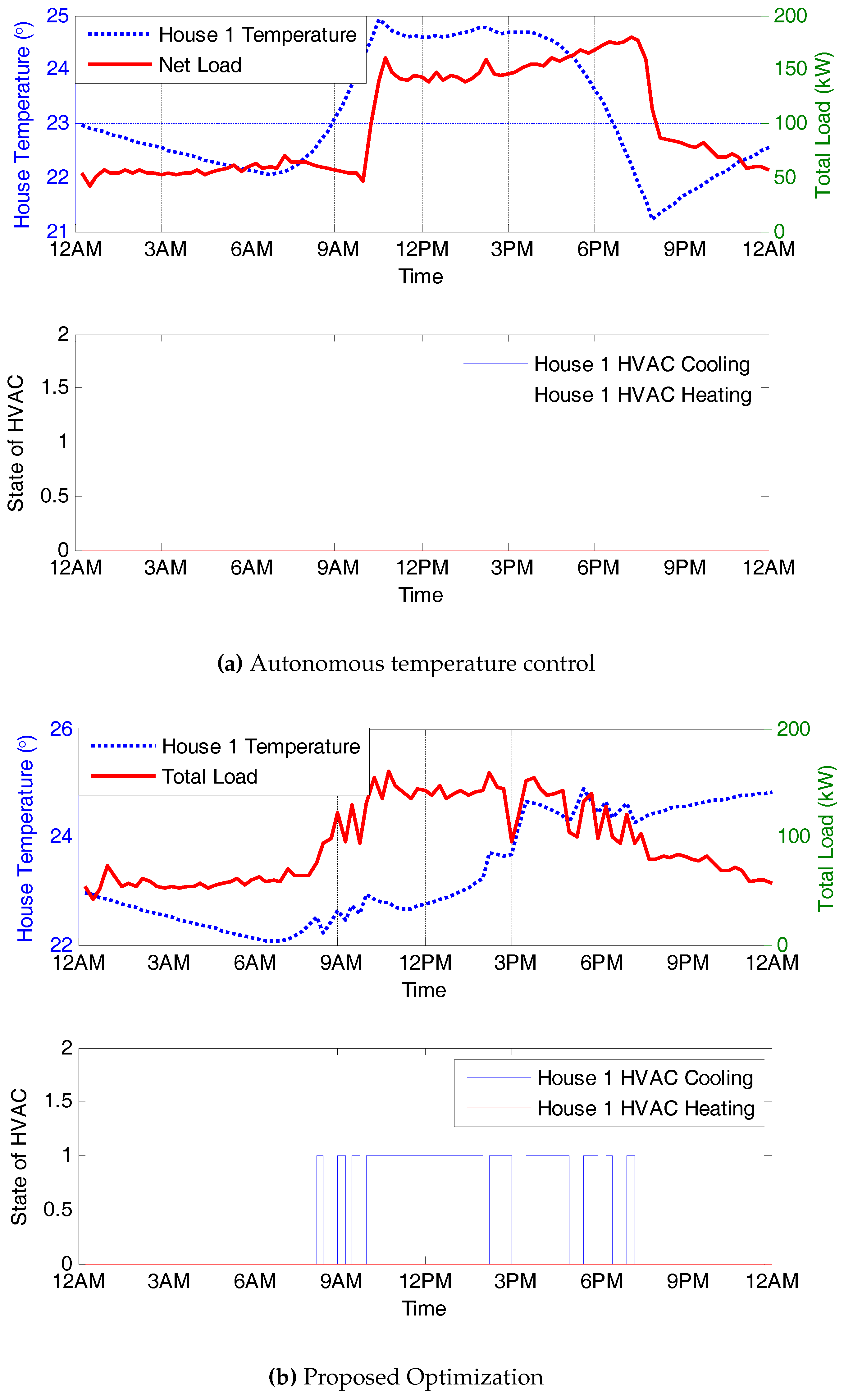
In this subsection,the results of autonomous temperature control and proposed D-OPF both in grid-connected mode are compared. Taking house # 1 for example, the indoor temperature and HVAC status are compared in Figure 5. Comparing Figure 5a with Figure 5b clearly shows how the proposed model considering can precool the house to reduce the HVAC consumption during peak price intervals. In specific, by the proposed optimization, the HVAC in house #1 is turned on before 9:00 a.m. when the indoor temperature is still comfortable. The house is precooled, so the HVAC can be turned off during the pick price intervals between 1:00 p.m.–2:00 p.m.
Figure 6 illustrates how the load is shifted by the proposed optimization comparing with the autonomous control method. As can be expected, the loads are shifted earlier in response to the price. Specifically, loads are shifted before the first price peak, so the second price peak can be avoided. With better thermal insulation of the house, the first price peak can also be avoided.
4.4. Operation in Islanded Mode
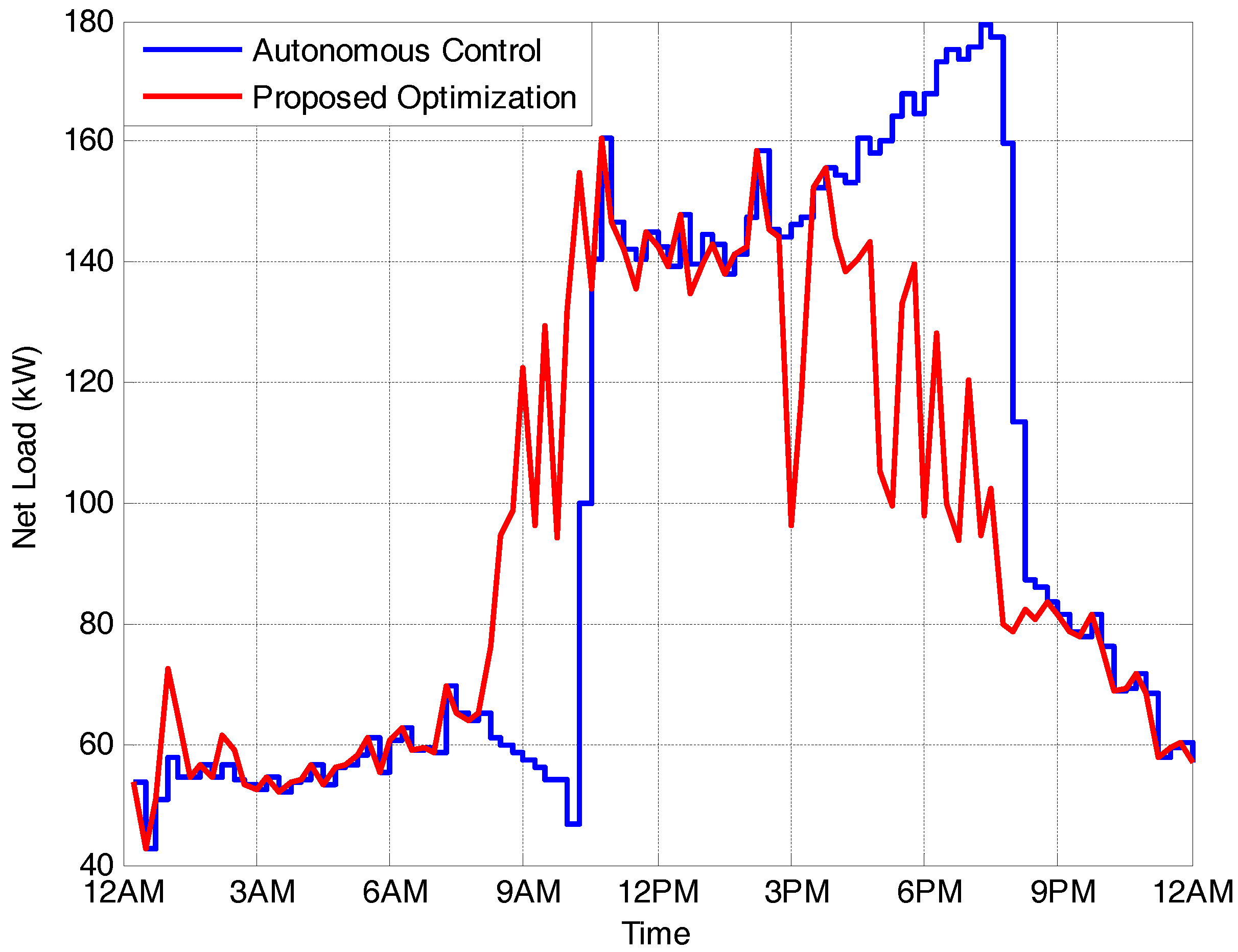
In this subsection,we compare the results of autonomous temperature control with proposed D-OPF both in islanded mode. The results are shown as in Figure 7. The net demand of the microgrid, i.e., the total load (both HVAC and non-HVAC) minus the renewable generation and shed load is found. With higher net demand, the electricity price will also be higher. This is because DGs with higher marginal cost need to be committed with additional net demand. Therefore, net demand is a good indicator of the electricity price. As can been seen in Figure 7a,b, the peak net demand of the proposed D-OPF model considering building thermal dynamics has been significantly reduced compared to that of autonomous control in islanded mode. This indicates the peak electricity prices of proposed D-OPF are reduced compared to that of autonomous control. Similar to the grid-connected cases, the proposed model can precool the house to reduce the HVAC consumption during peak price/demand intervals.
Figure 8 illustrates how load is shifted in islanded mode. As expected, the loads are shifted earlier to reduce both the value and duration of the peak load. In this way, units with higher marginal cost will be not committed or committed for a shorter time. Thus, the total operating cost will be reduced.
5. Conclusions
In this paper, an MICP-based community microgrid scheduling model considering building thermal dynamics and network operational constraints is proposed. The model directly integrates the detailed thermal dynamic characteristics of buildings into the optimization scheme and enables smart scheduling of HVAC systems. The proposed model optimizes both microgrid operating cost and system performance indices, such as network loss, voltage deviation and power factor at PCC. The proposed MICP model is validated on a ORNL microgrid test system by various simulations. Significant saving in electricity cost can be achieved with network operational constraints satisfied.
Acknowledgments
This work is supported by the U.S. Department of Energy’s Office of Electricity Delivery and Energy Reliability (OE) under Contract No. DE-AC05-00OR22725. This work also made use of Engineering Research Center Shared Facilities supported by the Engineering Research Center Program of the National Science Foundation and the Department of Energy under NSF Award Number EEC-1041877 and the CURENT Industry Partnership Program.
Author Contributions
Guodong Liu carried out the main research tasks and wrote the full manuscript. Thomas B. Ollis and Bailu Xiao contributed to the development of the proposed methodology and the literature review. Xiaohu Zhang and Kevin Tomsovic provided important suggestions on writing of the paper.
Conflicts of Interest
The authors declare no conflict of interest.
Nomenclature
The main symbols used in this paper are defined below. Others will be defined as required in the text. A bold symbol stands for its corresponding vector or matrix.
| Indices and Sets | |
| i | Index of DGs, running from 1 to . |
| b | Index of batteries, running from 1 to . |
| h | Index of houses, running from 1 to . |
| v | Index of PV generation, running from 1 to . |
| f | Index of feeders, running from 1 to . |
| n | Index of buses, running from 1 to . |
| t | Index of time periods, running from 1 to . |
| m | Index of energy blocks offered by DGs, running from 1 to . |
| Sets of DGs connected at bus n. | |
| Sets of batteries connected at bus n. | |
| Sets of houses connected at bus n. | |
| Sets of PV connected at bus n. | |
| Sets of feeders. | |
| Variables | |
| Binary Variables | |
| 1 if DG i is scheduled on during period t and 0 otherwise. | |
| 1 if HVAC of house h is scheduled cooling/heating during period t and 0 otherwise. | |
| 1 if battery b is scheduled charging/discharging during period t and 0 otherwise. | |
| Continuous Variables | |
| Power output scheduled from the m-th block of energy offer by DG i during period t. Limited to . | |
| Real/reactive power output scheduled from DG i during period t. | |
| Charging/discharging power of battery b during period t. | |
| Reactive power of battery b during period t. | |
| State of charge of battery b during period t. | |
| Real/ reactive power at PCC during period t. | |
| Real/reactive load of house h during period t. | |
| Real/reactive load curtailment of house h during period t. | |
| Indoor temperature of house h during period t. | |
| The temperature of thermal accumlating layer of inner walls and floor in house h during period t. | |
| The temperature of house envelop during period t. | |
| Voltage magnitude of bus n during period t. | |
| Real/ reactive power flow on line f during period t. | |
| Squared amplitudes of current on line f during period t. | |
| Constants | |
| Marginal cost of the m-th block of energy offer by DG i during period t. | |
| Purchasing price of energy from distribution grid during period t. | |
| Degradation cost of battery b during period t. | |
| Cost of load curtailment of house h during period t. | |
| Maximum/minimum output of DG i | |
| Maximum input/output power at PCC. | |
| Real/reactive power output from PV v during period t. | |
| Real/reactive power consumption scheduled for non-HVAC load in house h during period t. | |
| Rated power of HVAC system in house h. | |
| Maximum charging/discharging power of battery b. | |
| Maximum/minimum state of charge of battery b during period t. | |
| Maximum load curtailment of house h during period t. | |
| Battery charging/discharging efficiency. | |
| Customer discomfort cost of house h during period t. | |
| Allowed temperature deviation of house h during period t. | |
| Operating Cost of DG i at the point of . | |
| Ambient temperature during period t. | |
| Desired indoor temperature of house h during period t. | |
| Solar irradiance during period t. | |
| Thermal resistance between room air and ambient of house h. | |
| Thermal resistance between room air and the thermal accumulating layer in the inner walls and floor of house h. | |
| Thermal resistance between room air and the envelope of house h. | |
| Thermal resistance between the envelope of house h and the ambient. | |
| Total thermal capacitance of the indoor air of house h. | |
| Total thermal capacitance of the inner walls of house h. | |
| Total thermal capacitance of the house envelope of house h. | |
| The fraction of solar radiation entering the inner walls and floor of house h, then the rest of the solar energy is absorbed by the indoor air. | |
| Coefficient of performance (COP) of HVAC in house h. | |
| Maximum/Minimum voltage thresholds beyond which voltage deviation will be minimized. | |
| Maximum/Minimum voltage deviations. | |
| Apparent power limit of DG i, battery b and line f. | |
| resistance and reactance of line f. | |
| Maximum amplitudes of current on line f. | |
| Power factor limit of DG i. | |
| Power factor limits of battery b when charging/discharging. | |
| Power factor limits of PCC. | |
| Power factor of HVAC and non-HVAC load at house h. | |
References
- Lasseter, R.; Akhil, A.; Marnay, C.; Stephens, J.; Dagle, J.; Guttromson, R.; Meliopoulous, A.S.; Yinger, R.; Eto, J. CERTS Microgrid Concept. April 2002. Available online: https://pserc.wisc.edu/documents/research_ documents/certs_documents/certs_publications/certs_microgrid/certsmicrogridwhitepaper.pdf (accessed on 15 August 2017).
- Madureira, A.G.; Pecas Lopes, J.A. Coordinated voltage support in distribution networks with distributed generation and microgrids. IET Renew. Power Gener. 2009, 3, 439–454. [Google Scholar] [CrossRef]
- Beer, S.; Gomez, T.; Dallinger, D.; Momber, I.; Marnay, C.; Stadler, C. An economic analysis of used electric vehicle batteries integrated into commercial building microgrids. IEEE Trans. Smart Grid 2012, 3, 517–525. [Google Scholar] [CrossRef]
- Tsikalakis, A.G.; Hatziargyriou, N.D. Centralized control for optimizing microgrids operation. IEEE Trans. Energy Convers. 2008, 23, 241–248. [Google Scholar] [CrossRef]
- Agrawal, M.; Mittal, A. Microgrid technological activities across the globe: A review. Int. J. Res. Rev. Appl. Sci. 2011, 7, 147–152. [Google Scholar]
- Gu, W.; Wu, Z.; Bo, R.; Liu, W.; Zhou, G.; Chen, W.; Wu, Z. Modeling, planning and optimal energy management of combined cooling, heating and power microgrid: A review. Int. J. Electr. Power Energy Syst. 2014, 54, 26–37. [Google Scholar] [CrossRef]
- Belvedere, B.; Bianchi, M.; Borghetti, A.; Nucci, C.A.; Paolone, M.; Peretto, A. A microcontroller-based power management system for standalone microgrids with hybrid power supply. IEEE Trans. Sustain. Energy 2012, 3, 422–431. [Google Scholar] [CrossRef]
- Morais, H.; Kadar, P.; Faria, P.; Vale, Z.A.; Khodr, H.M. Optimal scheduling of a renewable micro-grid in an isolated load area using mixed-integer linear programming. Renew. Energy 2010, 35, 151–156. [Google Scholar] [CrossRef]
- Babazadeh, H.; Gao, W.; Wu, Z.; Li, Y. Optimal energy management of wind power generation system in islanded microgrid system. In Proceedings of the North American Power Symposium (NAPS), Manhattan, KS, USA, 22–24 September 2013. [Google Scholar]
- Palma-Behnke, R.; Benavides, C.; Lanas, F.; Severino, B.; Reyes, L.; Llanos, J.; Saez, D. A microgrid energy management system based on the rolling horizon strategy. IEEE Trans. Smart Grid 2013, 4, 996–1006. [Google Scholar] [CrossRef]
- Sobu, A.; Wu, G. Dynamic optimal schedule management method for microgrid system considering forecast errors of renewable power generations. In Proceedings of the 2012 IEEE International Conference on Power System Technology (POWERCON), Auckland, New Zealand, 30 October–2 November 2012. [Google Scholar]
- Mohamed, F.A.; Koivo, H.N. System modelling and online optimal management of MicroGrid using Mesh Adaptive Direct Search. Int. J. Electr. Power Energy Syst. 2010, 32, 398–407. [Google Scholar] [CrossRef]
- Cardoso, G.; Stadler, M.; Siddiqui, A.; Marnay, C.; DeFrost, N.; Barbosa-Povoa, A.; Ferrao, P. Microgrid reliability modeling and battery scheduling using stochastic linear programming. Electr. Power Syst. Res. 2013, 103, 61–69. [Google Scholar] [CrossRef]
- Nguyen, D.T.; Le, L.B. Optimal Bidding Strategy for Microgrids Considering Renewable Energy and Building Thermal Dynamics. IEEE Trans. Smart Grid 2014, 5, 1608–1620. [Google Scholar] [CrossRef]
- Liu, G.; Xu, Y.; Tomsovic, K. Bidding Strategy for Microgrid in Day-Ahead Market Based on Hybrid Stochastic/Robust Optimization. IEEE Trans. Smart Grid 2016, 7, 227–237. [Google Scholar] [CrossRef]
- Daratha, N.; Das, B.; Sharma, J. Coordination Between OLTC and SVC for Voltage Regulation in Unbalanced Distribution System Distributed Generation. IEEE Trans. Power Syst. 2014, 29, 289–299. [Google Scholar] [CrossRef]
- Dolan, M.J.; Davidson, E.M.; Kockar, I.; Ault, G.W.; McArthur, S. Distribution Power Flow Management Utilizing an Online Optimal Power Flow Technique. IEEE Trans. Power Syst. 2012, 27, 790–799. [Google Scholar] [CrossRef]
- Paudyal, S.; Canizares, C.A.; Bhattacharya, K. Optimal Operation of Distribution Feeders in Smart Grids. IEEE Trans. Ind. Electron. 2011, 58, 4495–4503. [Google Scholar] [CrossRef]
- Borghetti, A.; Bosetti, M.; Grillo, S.; Massucco, S.; Nucci, C.; Paolone, M.; Silvestro, F. Short-term scheduling and control of active distribution systems with high penetration of renewable resources. IEEE Syst. J. 2010, 4, 313–322. [Google Scholar] [CrossRef]
- Zhou, Q.; Bialek, J. Generation curtailment to manage voltage constraints in distribution networks. IET Gener. Transm. Distrib. 2007, 1, 492–498. [Google Scholar] [CrossRef]
- Calderaro, V.; Conio, G.; Galdi, V.; Massa, G.; Piccolo, A. Optimal Decentralized Voltage Control for Distribution Systems With Inverter-Based Distributed Generators. IEEE Trans. Power Syst. 2014, 29, 230–241. [Google Scholar] [CrossRef]
- Liu, G.; Ceylan, O.; Xu, Y.; Tomsovic, K. Optimal Voltage Regulation for Unbalanced Distribution Networks Considering Distributed Energy Resources. In Proceedings of the IEEE Power & Energy Society General Meeting (PESGM), Denver, CO, USA, 26–30 July 2015. [Google Scholar]
- Liu, G.; Xu, Y.; Ceylan, O.; Tomsovic, K. A new linearization method of unbalanced electrical distribution networks. In Proceedings of the North American Power Symposium (NAPS), Pullman, WA, USA, 7–9 September 2014. [Google Scholar]
- Shekari, T.; Golshannavaz, S.; Aminifar, F. Techno-Economic Collaboration of PEV Fleets in Energy Management of Microgrids. IEEE Trans. Power Syst. 2017, 32, 3833–3841. [Google Scholar] [CrossRef]
- Trakas, D.; Hatziargyriou, N. Optimal Distribution System Operation for Enhancing Resilience Against Wildfires. IEEE Trans. Power Syst. 2017, 99, 1. [Google Scholar] [CrossRef]
- Lavaei, J.; Low, S.H. Zero Duality Gap in Optimal Power Flow Problem. IEEE Trans. Power Syst. 2012, 27, 92–107. [Google Scholar] [CrossRef]
- Jabr, R. Radial distribution load flow using conic programming. IEEE Trans. Power Syst. 2006, 21, 1458–1459. [Google Scholar] [CrossRef]
- Baran, M.; Wu, F. Optimal capacitor placement on radial distribution systems. IEEE Trans. Power Syst. 1989, 4, 725–734. [Google Scholar] [CrossRef]
- Farivar, M.; Low, S. Branch flow model: Relaxations and convexification—Part I. IEEE Trans. Power Syst. 2013, 28, 2554–2564. [Google Scholar] [CrossRef]
- Nguyen, D.T.; Le, L.B. Joint optimization of electric vehicle and home energy scheduling considering user comfort preference. IEEE Trans. Smart Grid 2014, 5, 188–199. [Google Scholar] [CrossRef]
- Saaty, T. Decision making—The analytic hierarchy and network processes (AHP/ANP). J. Syst. Sci. Syst. Eng. 2004, 13, 1–35. [Google Scholar] [CrossRef]
- Thavlov, A. Dynamic Optimization of Power Consumption. Master’s Thesis, Technical University Denmark, Kongens Lyngby, Denmark, 2008. [Google Scholar]
- Madsen, H.; Holst, J. Estimation of continuous-time models for the heat dynamics of a building. Energy Build. 1995, 22, 67–79. [Google Scholar] [CrossRef]
- Bacher, P.; Madsen, H. Identifying suitable models for the heat dynamics of buildings. Energy Build. 2011, 43, 1511–1522. [Google Scholar] [CrossRef] [Green Version]
- Siroky, J.; Oldewurtel, F.; Cigler, J.; Privara, S. Experimental analysis of model predictive control for an energy efficient building heating system. Appl. Energy 2011, 88, 3079–3087. [Google Scholar] [CrossRef]
- Taylor, J.A.; Hover, F.S. Conic AC transmission system planning. IEEE Trans. Power Syst. 2013, 28, 952–959. [Google Scholar] [CrossRef]
- Baradar, M.; Hesamzadeh, M.R.; Ghandhari, M. Second-order cone programming for optimal power flow in vsc-type ac-dc grids. IEEE Trans. Power Syst. 2013, 28, 4282–4291. [Google Scholar] [CrossRef]
- Carrion, M.; Arroyo, J.M. A computationally efficient mixed-integer linear formulation for the thermal unit commitment problem. IEEE Trans. Power Syst. 2006, 21, 1371–1378. [Google Scholar] [CrossRef]
- Oak Ridge National Laboratory (ORNL) Rotating Shadowband Radiometer (RSR). Available online: https://www.nrel.gov/midc/ornl_rsr/ (accessed on 15 August 2017).
Figure 1.
Example community microgrid.
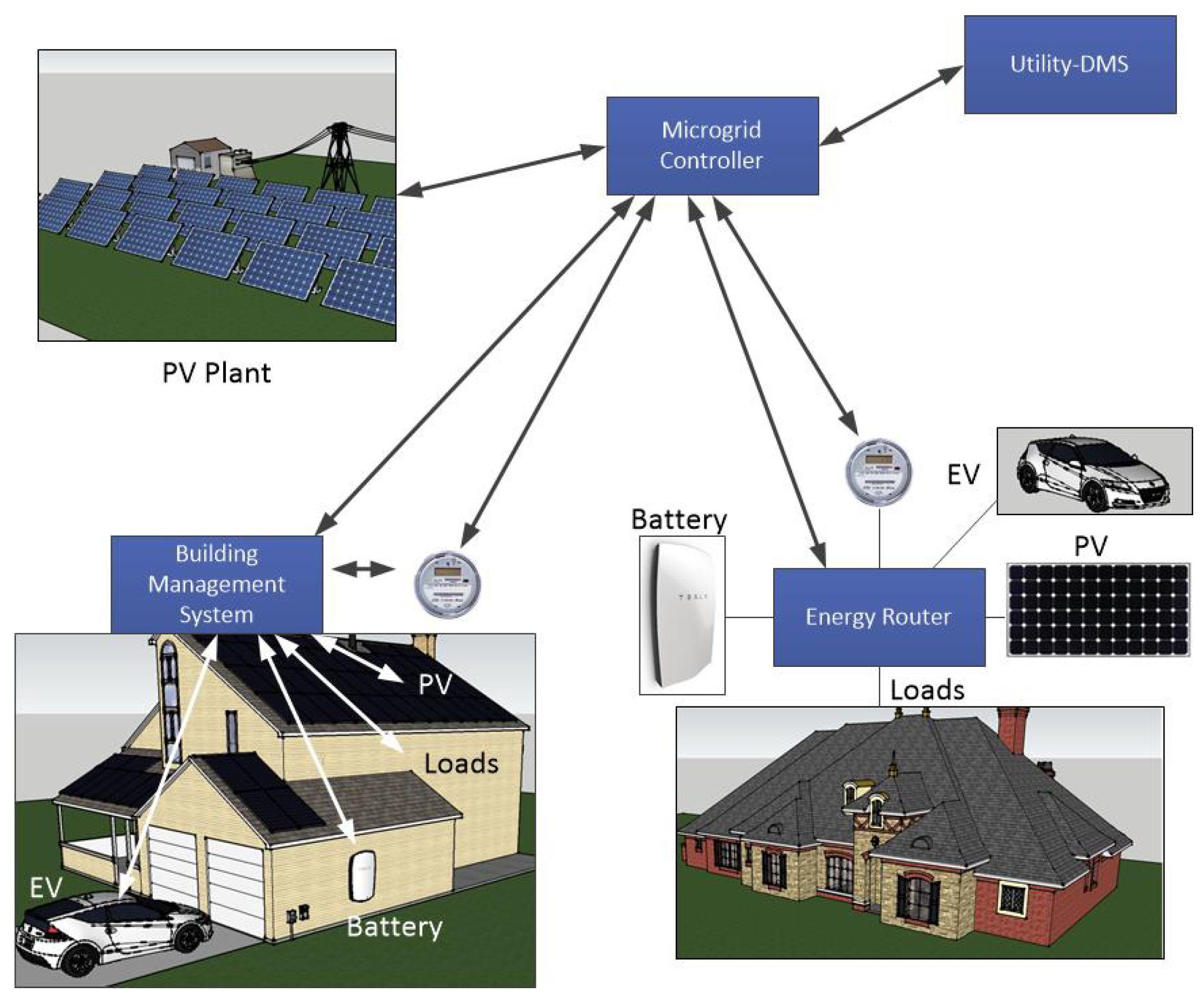
Figure 2.
Model of distribution feeder.

Figure 3.
Community microgrid test system.

Figure 4.
Non-HVAC demand in house and electricity price at the PCC.

Figure 5.
House temperature and HVAC status in grid-connected mode. (a) Autonomous temperature control by traditional thermostats in grid-connected mode; (b) Intelligent control by proposed optimization in grid-connected mode.
Figure 5.
House temperature and HVAC status in grid-connected mode. (a) Autonomous temperature control by traditional thermostats in grid-connected mode; (b) Intelligent control by proposed optimization in grid-connected mode.

Figure 6.
Load shifting in grid-connected mode.
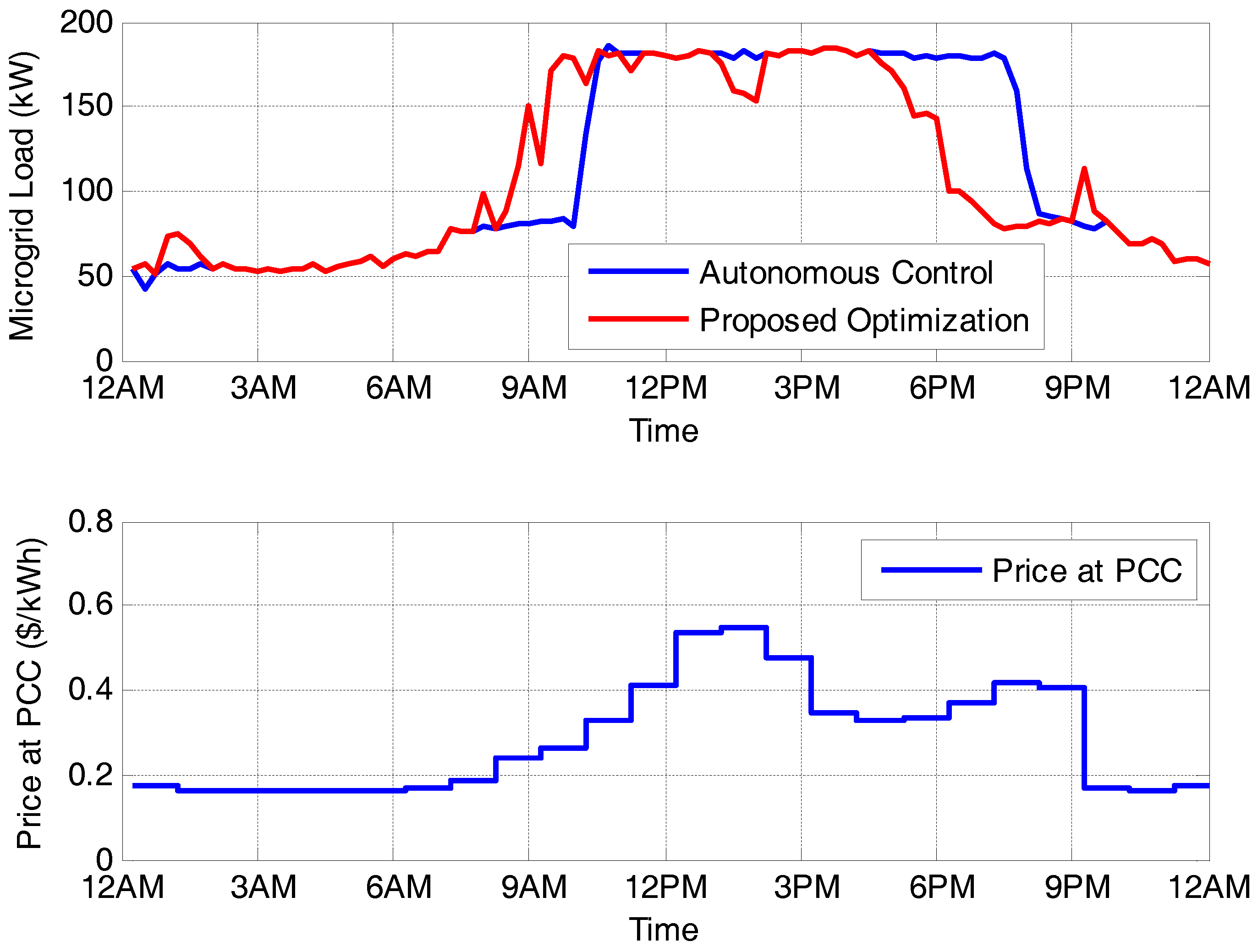
Figure 7.
House temperature and HVAC status in islanded mode. (a) Autonomous temperature control by traditional thermostats in islanded mode; (b) Intelligent control by proposed optimization in islanded mode.
Figure 7.
House temperature and HVAC status in islanded mode. (a) Autonomous temperature control by traditional thermostats in islanded mode; (b) Intelligent control by proposed optimization in islanded mode.

Figure 8.
Load shifting in islanded mode.


Table 1.
A typical pairwise comparison matrix terms.
| Total Cost | Total Reactive Power | Voltage Deviation | Network Loss | |
|---|---|---|---|---|
| Total Cost | 1 | 2 | 1/3 | 3 |
| Total Reactive Power | 1/2 | 1 | 1/5 | 2 |
| Voltage Deviation | 3 | 5 | 1 | 10 |
| Network Loss | 1/3 | 1/2 | 1/10 | 1 |
Table 2.
Comparison of the results between single objective optimization and multi-objective optimization for grid-connected operation.
Table 2.
Comparison of the results between single objective optimization and multi-objective optimization for grid-connected operation.
| Single Objective Optimization | Multiobjective Optimization | Autonomous Control | ||||
|---|---|---|---|---|---|---|
| Optimizing Cost | Optimizing Loss | Optimizing Voltage | Optimizing Reactive Power | |||
| Total Cost ($) | 521.49 | 661.38 | 558.65 | 584.27 | 531.73 | 634.75 |
| Loss (kWh) | 51.95 | 5.8197 | 14.6587 | 35.8221 | 25.77 | 23.59 |
| Voltage Deviation (pu) | 6.12 | 0.24 | 0.016 | 11.63 | 2.06 | 1.45 |
| Reactive Power (KVARh) | 242.14 | 0.11 | 0.05 | 0 | 0.06 | 0.04 |
Table 3.
Costs of the community microgrid in different cases.
| Cases | Total Objective | Operating Cost ($) | Loss (kWh) | Voltage Deviation (pu) | Reactive Power (kVARh) | |
|---|---|---|---|---|---|---|
| Grid-connected | Case 1: Autonomous Control | 134.66 | 634.75 | 23.59 | 1.45 | 0.04 |
| Case 2: Proposed Optimization | 113.70 | 531.73 | 25.77 | 2.06 | 0.06 | |
| Islanded | Case 3: Autonomous Control | 148.60 | 693.62 | 24.99 | 3.00 | 5.49 |
| Case 4: Proposed Optimization | 128.64 | 601.06 | 20.42 | 2.30 | 5.86 | |
© 2017 by the authors. Licensee MDPI, Basel, Switzerland. This article is an open access article distributed under the terms and conditions of the Creative Commons Attribution (CC BY) license (http://creativecommons.org/licenses/by/4.0/).
Share and Cite
MDPI and ACS Style
Liu, G.; Ollis, T.B.; Xiao, B.; Zhang, X.; Tomsovic, K. Community Microgrid Scheduling Considering Network Operational Constraints and Building Thermal Dynamics. Energies 2017, 10, 1554. https://doi.org/10.3390/en10101554
AMA Style
Liu G, Ollis TB, Xiao B, Zhang X, Tomsovic K. Community Microgrid Scheduling Considering Network Operational Constraints and Building Thermal Dynamics. Energies. 2017; 10(10):1554. https://doi.org/10.3390/en10101554
Chicago/Turabian StyleLiu, Guodong, Thomas B. Ollis, Bailu Xiao, Xiaohu Zhang, and Kevin Tomsovic. 2017. "Community Microgrid Scheduling Considering Network Operational Constraints and Building Thermal Dynamics" Energies 10, no. 10: 1554. https://doi.org/10.3390/en10101554
Note that from the first issue of 2016, this journal uses article numbers instead of page numbers. See further details here.