1. Introduction
Modern distribution systems are characterized by the simultaneous presence of renewable energy sources, storage systems and loads that actively contribute to the operation of such systems, along with an increasingly complex and performing information and communications technology relevant infrastructure. In this context, power quality (PQ) is one of the most important issue since adequate PQ levels guarantee the necessary compatibility among all equipment connected to the grid [
1]. Among PQ disturbances, the waveform distortions are considered with much attention as a consequence of several factors such as: (1) the sensitivity of customers to such disturbances and (2) the growing penetration of electrical components responsible for new and significant waveform distortions.
Recently, renewable energy sources, especially wind and solar energy, and some high-efficiency end-user devices, e.g., fluorescent lamps powered by high-frequency ballasts, have attracted great interest as perturbing devices since they contribute significantly to increasing the distortion levels of voltage and current waveforms [
2,
3,
4]. They have a spectrum that includes a wide range of frequencies that can exceed 2 kHz up to 150 kHz. This spectral content was initially indicated as “high-frequency distortion”, but recently the term “supraharmonic” was introduced [
5] and it is being used more frequently [
2,
6,
7,
8].
The presence of these high-frequency spectral components can cause different problems in the electrical power systems, such as: (i) the potential interferences with the power-line communication (PLC), that are included in the same range of frequency [
7,
8], or rather; (ii) the possible appearance of both series and parallel resonance phenomena [
9,
10,
11] and (iii) the impact of this distortion on end-user equipment and on equipment in the grid [
5,
7,
8,
9]. Obviously, the aforesaid problems may be overcome with the exact knowledge of the high-frequency spectra in terms of both amplitude and frequency spectral components versus time, also when an active filtering has to be provided for their compensation [
10]. However, these high-frequency spectral components are superimposed to low frequency spectral components with consequent conflicting needs in term of time window length (and frequency resolution) for their spectral analysis.
Moreover, such high-frequency disturbances still require not only appropriate analysis tools, but also adequate standardizations, which allow to define proper indices and their maximum thresholds for the evaluation and the limitation of the high-frequency spectral components. Note that the importance of covering the frequency range from 2 kHz to 150 kHz with adequate standards was also underlined in a European Committee for Electrotechnical Standardization (CENELEC) report, in the International Electrotechnical Commission (IEC) standard TS 62749, by different Conseil International des Grands Réseaux Électriques (CIGRE)/Congrès International des Réseaux Electriques de Distribution (CIRED)/Institute of Electrical and Electronic Engineers (IEEE) working group and in the application guide for the EN50160. Moreover, several international standard setting organizations are working on this topic [
2,
5,
6,
7].
As well known, currently, the IEC standards, which address the range from 0 kHz to 9 kHz, recommend for signal processing the use of the discrete Fourier transform over successive and rectangular time windows with a duration fixed as an integer multiple of the fundamental period, also called short time Fourier transform (STFT) [
4,
12]. The STFT method, together with the other STFT-based ones, has been proved to be an important tool for the global evaluation of waveform distortions, but it cannot provide more detailed information about each spectral component. This is due to the inaccuracies associated with the inherent fixed frequency resolution and spectral leakage problems. Moreover, in case of waveforms characterized by wide spectra, these problems became more significant due to the aforementioned different behaviours of low- and high-frequency spectral components and the increasing desynchronization of high-frequency components. As attempt to reduce STFT inaccuracies, IEC suggests the use of grouping not only for the low frequency range, but also for the spectral content from 2 kHz to 9 kHz, assuming high-frequency resolution to be unnecessary for this range, in opposition to the modern requirements [
13,
14]. Recently, in [
14], some measurement methods have been also indicated to provide an overview of spectral content in the range from 2 kHz to 150 kHz, as opposed to detailed measurement methods used for low-frequency range. These measurement methods for the high-frequency spectral components are informative and not normative; they include the extension of the grouping from 9 kHz to 150 kHz using a 10 Hz frequency resolution and 200 Hz bands to group this spectral content [
14] and, then, do not allow to obtain acceptable estimations of amplitudes and frequencies of high-frequency spectral components.
The IEC standard [
14] suggests also the use of measurement methods according to Comité international spécial des perturbations radioélectriques CISPR 16-1-2 for the evaluation of the high-frequency spectral content; however, it states also that it is not always possible or practical to apply them. In fact, these measurement methods suffer of complex and expensive implementation; also, they provide an enormous amount of data to be stored as output. Moreover, IEC standard highlights that the measurement methods according to CISPR 16-1-2 focus only on emissions from devices under test, stating that they are “
not directly addressed to power quality investigations”. Hence, the IEC standard suggests also the use of other techniques for the analysis of the high-frequency spectral content and advises about the possible inclusion of other methods in future editions of the standard.
However, with reference to the low frequency range, to solve the problems associated with the IEC standard method, many spectral analysis methods have been presented in the relevant literature for the assessment of time varying waveform distortions [
4,
12,
14,
15,
16,
17]. Among them, wavelet-based methods are introduced as an alternative tool, exploiting the wavelet insensitive behaviour to the frequency fluctuations. Moreover, several advanced parametric methods has also been proposed, such as the sliding-window estimation of signal parameters by rotational invariance technique (ESPRIT) method and the sliding-window Prony’s method. Although these parametric methods are characterized by enhanced accuracy and great frequency resolution, their computational burden is excessive. In recent literature, hybrid sliding-window parametric-STFT methods and new modified sliding-window parametric methods have been proposed to reduce the computational effort [
14,
15,
16,
18,
19]. With reference to the high-frequency range, in the relevant literature, only few methods were applied to the spectral analysis of waveforms with wide spectra [
15,
16]. In particular, the method proposed in [
16] was not applied for the simultaneous spectral analysis of the entire range from 0 Hz to 150 kHz. It requires a high computational effort and a priori knowledge of the number of spectral components included in the analysed waveform, as well as the order of the correlation matrix. These two problems were overcome by the method proposed in [
15], although it was not applied for the detection of high-frequency time varying spectral component, when large-spectrum waveforms are analysed.
Note also that low frequency spectral components and high frequency spectral components can be characterized by different behaviours in the frequency and time domain; low frequency components can be stationary while high frequency are usually not stationary.
Motivated by these issues, the new contribution of this study is in proposing a novel scheme to analyse electrical waveforms with spectral content up to 150 kHz that provides accurate estimation of parameters (mainly, frequencies, amplitudes and initial phases) of spectral components, while maintaining acceptable computational efforts. The proposed method allows to have an accurate contemporary knowledge of low and high frequency spectral components and their time behaviour; thus, it is useful for:
the evaluation of supraharmonic emission;
the definition of adequate power quality indices to introduce standard methods and limits;
the study of supraharmonic propagation and impact in power systems;
the definition of new models which can emulate supraharmonic injection;
the use of proper adaptive active filters to reduce the emission of supraharmonics.
Based on the previously-cited main aspects of the spectral analysis methods offered by relevant literature, the proposed method applies a discrete wavelet transform (DWT) and a sliding-window modified ESPRIT method (SW MEM) [
15] in two successive steps. The DWT divides the original signal into low-frequency and high-frequency waveforms. The SW MEM separately analyzes the two passbands for a separate estimation of the low-frequency and high-frequency spectral components.
The application of the proposed method has the following advantages:
it allows a detailed estimation in time of each high-frequency spectral component;
it has ability to provide the optimal time and frequency resolutions in each band to obtain an accurate time-frequency representation using the strategy of divide and conquer.
Eventually, we evidence that the main contribution of this paper refers to the application addressed (signal processing in power distribution systems in the entire frequency range) since the spectral analysis of waveforms in electrical distribution systems with wide spectra (including supraharmonics) is nowadays of the greatest interest. Moreover, even though the proposed scheme uses basic and well known methods, these methods are used in a novel and advantageous way.
This article is organized as follows:
Section 2 introduces some considerations on the high-frequency components up to 150 kHz to outline their main spectral characteristics. In
Section 3, the new sliding-window wavelet-modified ESPRIT-based method (SWWMEM) is described in detail.
Section 4 describes how the numerical validation of the proposed method is affected. The study conclusions are in
Section 5.
2. Spectral Components in the Range from 2 kHz to 150 kHz
Nowadays, the main cause of waveform distortions in modern electrical power systems is the growing use of devices equipped with static converters. They can inject in the grid distorted currents with spectral components included in a wide frequency range (up to 150 kHz) [
3,
4,
16,
20]. In order to better underline how the problem of the waveform distortions that involve a wide frequency range is deeply rooted in modern electrical power systems, a detailed list of common supraharmonic emitters is provided in [
21]. These are: (i) converters for industrial applications that mainly emit spectral components in the range from 9 kHz to 150 kHz; (ii) oscillation related to the electronic device commutation that mainly emit spectral components up to 10 kHz; (iii) street lamps that mainly emit spectral components up to 20 kHz; (iv) electro-vehicle chargers that mainly emit spectral components in the range from 15 kHz to 100 kHz; (v) photovoltaic and wind turbine inverters that mainly emit spectral components in the range from 4 kHz to 20 kHz; (vi) household devices, e.g., liquid-crystal display televisions or highly-efficient loads, that mainly emit spectral components in the range from 2 kHz to 150 kHz; (vii) PLC that mainly emit spectral components in the range from 9 kHz to 95 kHz.
Since, as seen, the supraharmonic emitters are very common the spectral components from 2 kHz to 150 kHz have recently received great interest in the relevant literature [
2,
7,
16,
20,
21,
22,
23,
24,
25,
26,
27]. Many research activities have recently focused on the effects of the high-frequency sources on the power systems and their propagation [
2,
6,
7]. These studies discerned between primary and secondary emissions. Primary emissions refer only to the distinctive disturbances of the considered load or production equipment. Secondary emissions refer to the disturbances caused by other sources near the considered equipment. Moreover, it was outlined that the frequencies from 2 kHz to 150 kHz are strictly linked to the switching technique adopted in the interfacing power-electronic converter. Several measurements taken by low power (up to 100 kW) equipment indicate that the most common switching frequencies are up to few tens of kHz [
28]. Note that, sometimes, the secondary emission might also be due to PLC, they, as previously observed, generally work in the range from 9 kHz to 95 kHz and interferences could occur in the power system [
8].
The main difference between the high-frequency emissions and low-frequency emissions is that, while the latter tend to propagate towards the distribution network, the former mainly flow within the installation, towards the other devices that offer a lower impedance than the network at so high frequencies (such as the electromagnetic compatibility (EMC) filter). Moreover, the presence of EMC filter as interface at the point of common coupling (PCC), also provides a low impedance for these high-frequency components coming from the distribution network. Therefore, high-frequency currents from both the installation and the network flow through the capacitor, causing high-frequency voltage distortion at the PCC [
6].
Most of waveforms with spectral components from 0 kHz to 150 kHz are related to distributed generation (DG) and loads equipped with static converters.
With reference to DGs emission, photovoltaic systems (PVSs) and wind turbine systems (WTSs) are the more spread technologies and they generally are connected to the grid through power static converters [
28]. Thus, high-frequency components are introduced at the PCC as primary emissions by the interfacing converters.
In PVSs, the high-frequency primary emission is linked to the adopted pulse-width modulation (PWM) technique of the inverter, although the presence of the electromagnetic interference (EMI) filter, used to reduce the harmonic emission, influences the amplitude of the high-frequency components with respect to an ideal PWM spectrum [
7]. The high-frequency components can be detected in ideal operating conditions of the system, in correspondence of the frequencies
, given by:
where
is the switching frequency and
is the power system fundamental frequency. They are sidebands centered on integer multiples of the switching frequency, which is generally a few tens of kHz.
Regarding the WTSs, the schemes equipped with a power static converter are the doubly fed induction generator (DFIG) and the full-scale power converter wind turbine [
29]. For both these configurations, the power electronic converter is the main source of high-frequency primary emissions at the PCC.
The high-frequency secondary emissions at the PCC of both PVSs and WTSs are due to background voltage distortion and could increase significantly in the presence of resonance effects [
20].
With reference to loads emission, several types of perturbing loads can introduce high-frequency components [
7,
8,
30,
31]. In particular, the propagation of high-frequency components as primary emissions of adjustable speed drives (ASDs) with a 6 kHz switching frequency in industrial networks has been analyzed in [
31]. In [
7] it was outlined that the electrical vehicles (EVs) produce a weak primary emission at low frequencies, while in the high-frequency range, the levels of current emission can be significant. Moreover, in the measured currents at the PCC of EV chargers, spectral components in a range from 10 kHz to 100 kHz have been detected [
7].
The most diffuse disturbing loads are currently the fluorescent lamps powered by high-frequency ballast and the LED lamps [
7,
8]. Generally, an electronic ballast has a voltage stiff rectifier (which create harmonics) and also an inverter that is normally switching at constant frequency (typically from 30 kHz to 40 kHz). Components in both these frequency ranges can be measured at the grid side of the lamps as a emission in the current. In addition, since lamps larger than 25 W have to improve the harmonic emission, an active power factor correction (APFC) stage is placed directly after the rectifier. This is typically done with a DC to DC converter that make sure that the current drawn by the lamp is almost sinusoidal. However this means that there is an additional source of emission that changes amplitude and frequency over the fundamental cycle. The frequency emission from this part of the lamp is shifting from 30 to 40 kHz to 100 kHz over half of a fundamental cycle [
32].
The high-frequency secondary emission at the PCC of the aforesaid loads are generally caused by background voltage or by the presence of several non-linear loads in the same installation.
3. The Proposed Method
In the most general case, a waveform in a power system can be characterized by both high-frequency and low frequency (up to 2 kHz) spectral components involving conflicting needs in term of time window length and frequency resolution for their spectral analysis.
The high-frequency spectrum is generally characterized by spectral components centred around frequencies not directly linked to the power system frequency and that are commonly defined as “asynchronous” components. The low frequency spectral components are mainly constituted by discrete components at frequencies that are linked to the power system frequency [
6,
7]. Moreover, high-frequency and low-frequency spectral components present different time behaviours, being high-frequency components often not stationary with fast dynamics, and consequently with frequencies and amplitudes that can rapidly vary vs. time. Finally, in the absence of resonance effects, the energy content of high-frequency components usually is very small if compared with the characteristic low-frequency spectral components.
Eventually, the spectral analysis of waveforms including both low-frequency and high-frequency spectral components requires an approach different from the traditional approach for the low-frequency components only. In particular, the method to be used should be characterized by the ability to:
separate the original signal in different frequency bands;
analyze different frequency bands with different time and frequency resolutions;
analyze different frequency bands with adequate accuracy for different levels of distortions estimating both amplitude and frequency of each spectral component in time.
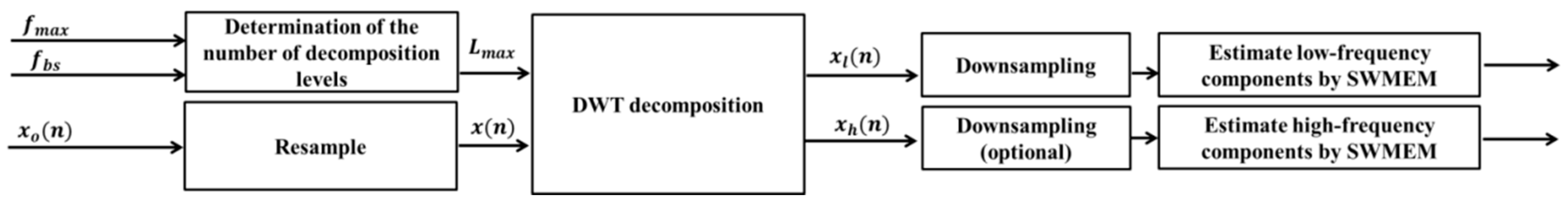
Motivated by above, the main features of the proposed method are (1) to isolate the different frequency bands of interest and (2) to separately analyse each band, taking into account the different behaviour and needs of low-frequency and high-frequency components (
Figure 1).
The proposed method involves a two-step procedure as shown in
Figure 1. In particular, the selected values
and
are the bands’ separation frequency and the maximum frequency of interest, respectively. In the first step, the number of decomposition levels is calculated, the waveform is adequately resampled and then filtered by the decomposition of a discrete wavelet transform (DWT), which produces a low-frequency band and a high-frequency band of the original waveform. Then in the second step, the two parts of the waveform are resampled and analyzed separately by the sliding-window modified ESPRIT method (SW MEM).
In the first step, we take the advantage of wavelet suitability for studying signals in different frequency bands with different frequency resolution [
33,
34]. Moreover, the DWT, differently to a common low/band-pass filter, performs a waveform decomposition that guarantees no phase-shifting and no signal leakage among the decomposed bands of frequency. This allows that, if all of the reconstructed signals of the different bands of frequency are added up, the original waveform is again obtained. In the second step, we use ESPRIT method which is one of the most accurate parametric methods; in particular: (i) ESPRIT method performs better than Prony’s method when the waveform to be analysed is corrupted by noise; (ii) DWT can be couplet better with ESPRIT method than with other parametric methods; in fact, if
is the waveform sampling rate, ESPRIT method, as well as DWT, is able to detect spectral components up to
. In the following subsections, the main features of each of these steps are described in detail.
3.1. First Step
The first step of the proposed hybrid method is based on the application of a DWT obtained by using a sampled mother wavelet with discrete scale and translation parameters, applied to a sampled waveform [
12].
Specifically, given a sequence of samples
with
and the chosen continuous mother wavelet
with
and
continuous scale and translation parameters respectively, selecting
and
, the sampled discrete mother wavelet
is:
where
and
are integers and the values
,
are fixed [
12]. Hence, the DWT of
is provided by:
where the symbol * indicates the complex conjugate [
12].
It is well known that the DWT achieves the decomposition of the waveforms on different levels. Two parts are obtained for each level and they represent the approximation
and the detail
of the waveform in progressively-halved bands of frequency. In particular, by defining the scaling function
as the aggregation of wavelets with scale factor
, and discretizing it as seen for the mother wavelet, at each level
, the approximation
and the detail
of the original waveform can be evaluated by the inverse DWT of the approximate
and detailed
coefficients, computed as follows:
where
is related to the translation in time and
is related to the selected frequency band [
12].
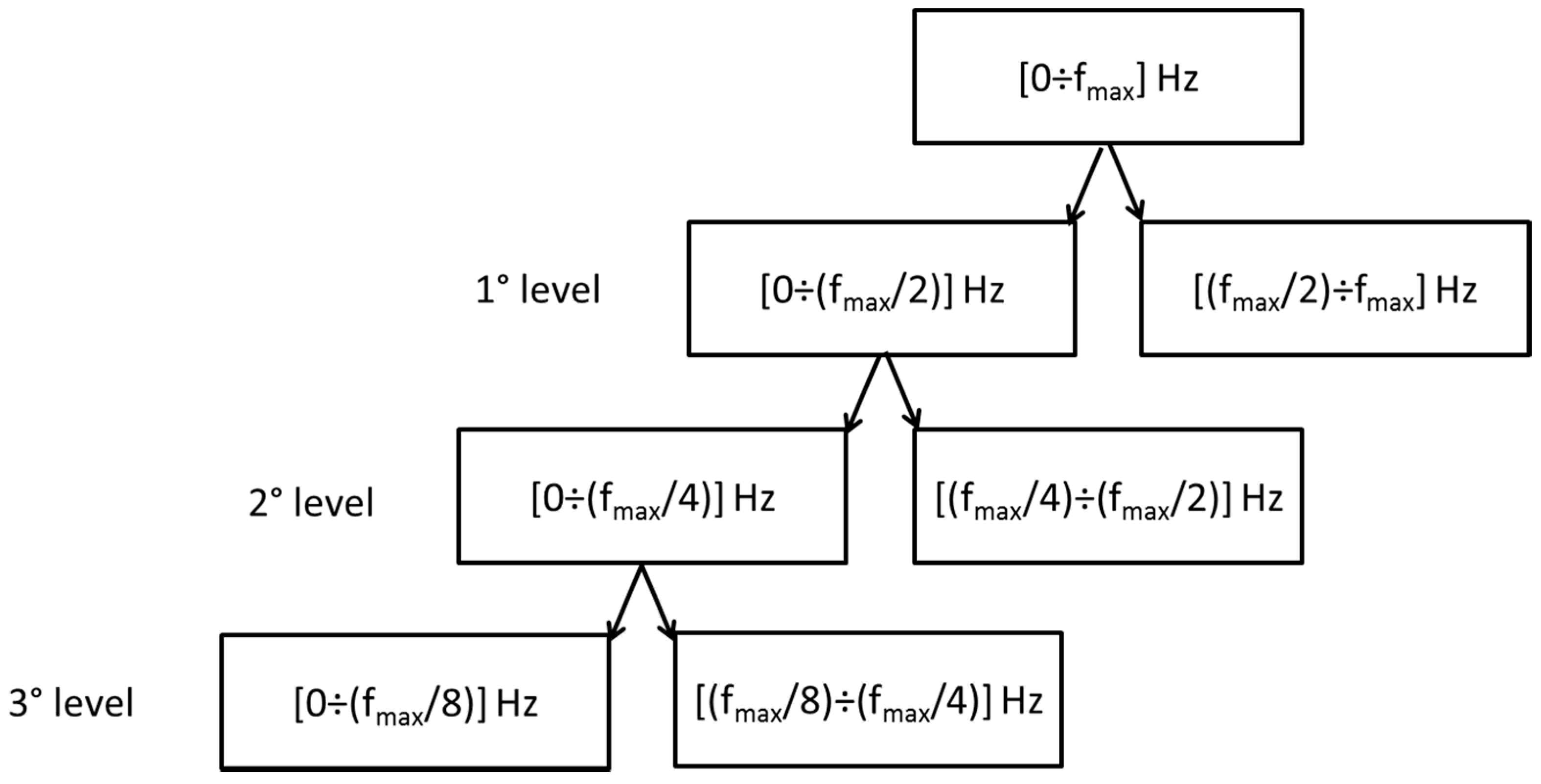
Figure 2 shows a representation of the DWT decomposition for a waveform sampled at
Hz, where
is the maximum frequency of interest (i.e., 150 kHz).
The DWT decomposition is often used as a filter bank, since it appears a sort of high and low pass band filters in cascade, with two bands of frequency obtained at each level. However, the bands are affected by overlap and attenuation at their edges. In the proposed method, by using a Meyer mother wavelet, multi-level DWT decomposition is achieved by assuming, as the number of decomposition levels, a value that depends on and on the bands’ separation frequency (i.e., 2 kHz), i.e., , where the symbol indicates the rounding up operation.
Note that as shown in
Figure 1, the original waveform
to be analyzed can be pre-processed to adapt the sampling frequency to the maximum frequency of interest
, obtaining the DWT input waveform
. This pre-processing consists in an upsampling of
, in order to avoid filter bounds to be too close to the frequencies that must be detected.
Once the DWT decomposition is known, two different waveforms,
and
, are obtained. They are the waveform
(“low-frequency waveform”), which includes only the approximation
at the level
(
Figure 2) and the waveform
(“high-frequency waveform”), which includes the sum of all of the details
(
Figure 2). The level
instead of
was chosen to avoid the attenuation effects of the overlap introduced by the canonical DWT in the ranges of frequencies of interest.
Both the low-frequency waveform
and the high-frequency waveform
are separately analyzed in the second step of the proposed method (
Figure 1).
3.2. Second Step
The second step of the proposed hybrid method is based on the application of the sliding-window modified ESPRIT method (SW MEM) described in [
15]. This method is applied for the assessment of the low-frequency and high-frequency components included in
and
, respectively.
Specifically, denoting with
, of generic size
, either the sequence of the
-sized sampled data
or the sequence of the
-sized sampled data
(
Figure 1), the ESPRIT model is used to approximate the waveform samples with a linear combination of
complex exponentials added to a white noise
[
12]:
where
is the sampling period and
,
,
, and
are the amplitude, initial phase, frequency and damping factor of the
kth complex exponential, respectively. These are the unknown parameters to be estimated by using the transformation properties of the rotation matrix associated with the waveform samples. However in [
15], it was shown that a reduction of the unknown parameters in the model (5) is possible, considering that the damping factors and the frequencies of spectral components in power system applications generally vary slightly vs. time, especially at low-frequencies. This is the basic principle of the SW MEM, where the estimation of frequencies and damping factors is realized only a reduced number of times along the whole waveform to be analyzed, with a great improvement in terms of computational effort [
15]. In particular, the frequencies of the spectral components are initially evaluated in the first sliding window (also called “basis window”). Then the obtained values are assumed to be known quantities in the successive sliding windows (also called “no-basis windows”). The same handling is also performed for the damping factors.
Note that a check is conducted in each no-basis window to evaluate if the frequencies and damping factors obtained in the basis window can be still considered valid. In particular, the reconstruction error of the waveform can be checked; if the reconstruction error is greater than a fixed threshold, a new basis window is generated, the frequencies and the damping factors are updated and these new values are imposed in the following no-basis windows [
15]. This check makes the SW MEM also suitable for the high-frequency components assessment, since they might significantly vary vs. time as previously mentioned.
The accuracy of the results and the computational effort of the SW MEM are influenced significantly by the number of exponentials,
, by the selected order
of the correlation matrix and by the sampling frequency
[
14].
In particular, it is worthwhile to outline the following considerations:
- (1)
Thanks to the DWT decomposition in the first step, both and include a reduced number of spectral components than the original sequence , so the analyses of these waveforms require smaller values of than the analysis of the original sequence .
- (2)
Since include only high-frequency components, the duration of the analysis window for this waveform can be chosen shorter than that for the spectral analysis of , consequently reducing the value of .
- (3)
Since the maximum frequency that the ESPRIT method and therefore the SW MEM are able to detect is half of the sampling frequency
[
14]. The low frequency waveform
can be downsampled to only
(two times the bands’ separation frequency), reducing the number of samples in each window and, once again, the global computational burden.
Note also that to prevent the problem associated with the attenuation introduced by the DWT decomposition, only the spectral components over (i.e., 2 kHz) were stored when analyzing , whereas the spectral components up to were stored when analyzing .
Finally, it is important to observe that since the duration of window for the spectral analysis of is shorter than that for the spectral analysis of , the proposed method could provide a number of high-frequency spectra greater than the number of spectra of the low-frequency waveform. This result is in accordance with the need for having a higher time resolution for the detection of the high-frequency components, since these components generally vary vs. time more than the low-frequency components.
4. Numerical Validation of the Proposed Method
Several numerical analysis of synthetic and measured waveforms in different operating conditions of typical generation systems and loads were performed. For sake of conciseness, only three case studies are shown in this Section. Specifically, the first two case studies analyse synthetic waveforms while the third case study is an actual waveform measured at the PCC of fluorescent lamps installation. In order to test the effectiveness of the proposed hybrid method (SWWMEM) in terms of both computational burden and accuracy, the same waveforms were analyzed also through the STFT method (STFTM), selecting a 5 Hz frequency resolution, and through the Sliding-Window ESPRIT method (SWEM) [
12].
Moreover, also the spectrogram presented in [
23] is included for all of the considered case studies, in order to underline the different approach of SWWMEM in respect to the currently available high-frequency signal processing technique.
All of the waveform analysis were performed in MATLAB environment. The MATLAB programs were developed and tested on a Windows PC with an Intel i7-3770 3.4 GHz and 16 GB of RAM.
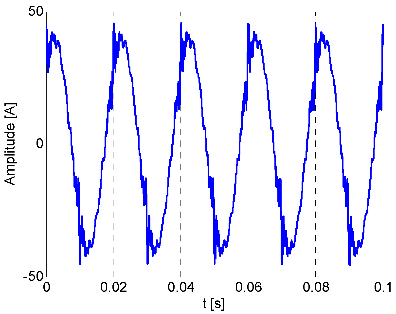
4.1. Case Study 1
A synthetic 3 s waveform that emulates a current at the PCC of a PV system equipped with a full-bridge, unipolar inverter, is analyzed (
Figure 3). Specifically, the waveform was assembled assuming a fundamental current of 40 A at 50.02 Hz and a frequency modulation index
mf of the inverter PWM technique equal to 200; then all odd harmonics up to the 27th order (low-frequency components) and a white noise with a standard deviation of 0.001 were added.
The sampling frequency of the waveform was 50 kHz, in order to provide the most appropriate operating conditions for the parametric methods; this choice allowed the detection of the spectral components around the order 2
mf, that are the most significant introduced by the inverter PWM and whose amplitudes were fixed up to 2% of the fundamental, in order to emulate the behavior of the PV system during high-irradiance conditions [
35].
A resampling to 100 kHz was required in the first step of the proposed method, in order to guarantee an uncorrupted estimation of the spectral components of our interest. Moreover, fixing the bands’ separation frequency equal to 2 kHz, the number of decomposition levels was 5.
For the SWEM, the error threshold was fixed equal to 10−5, and the window of analysis moves by 0.04 s without overlap. The same setting was chosen also for the spectral analysis of the low-frequency waveform (downsampled to 5 kHz) through the SWWMEM. For the analysis of the high-frequency range waveform, instead, the error threshold was fixed equal to 10−4, and the window of analysis moves by 0.018 s without overlap.
Table 1 shows the average percentage errors of the frequencies (
Table 1a) and of the amplitudes (
Table 1b) for five selected spectral components. These spectral components are the fundamental, the 3rd and the 11th harmonic (low-frequency components) and two components (
and
) linked to the inverter switching frequency (high-frequency components). The proposed method seems to outperform the STFTM, since it provides average percentage errors that are globally very similar to those obtained by the SWEM, both for amplitude and frequency estimation.
In particular, for the low-frequency spectral components, the errors of SWWMEM are slightly lower than that of SWEM, while the proposed method provides average percentage errors on frequency and amplitude that are two and three orders of magnitude lower than those obtained through the STFTM.
For the high-frequency components, the average percentage errors on the amplitudes obtained by the proposed method show a significantly improved accuracy compared to the errors obtained through STFTM; in fact, STFTM errors are greater than 82% and are affected by spectral leakage problems that increase as the frequency increases. Also in this range of frequencies, the SWWMEM provides errors very close to the SWEM errors, and they do not exceed 0.09% in amplitude and 2.5 × 10⁻⁵% in frequency. Similar mean errors were observed for all the spectral components of the whole waveform using both the SWWMEM and the SWEM. However, the proposed method generally seemed to produce slightly lower amplitude mean errors than SWEM.
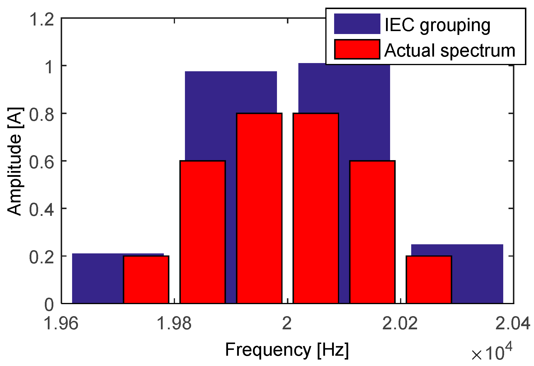
Note that also the grouping, recommended by the IEC, both for the low-frequency components (using a 200 ms analysis window) and for the high-frequency components (using a 100 ms analysis window) was evaluated. This post-processing provides, for the low-frequency components, percentage errors on the amplitude practically coincident with the values obtained for the STFTM in
Table 1. Conversely, for the high-frequency components, the grouping provides an aggregation of spectral components centered around fixed frequencies equal to 19.9 kHz and 20.1 kHz, as shown in
Figure 4. It is clear that at high-frequency, this aggregation allows only to detect approximatively the allocation of the energetic content around the fixed frequencies.
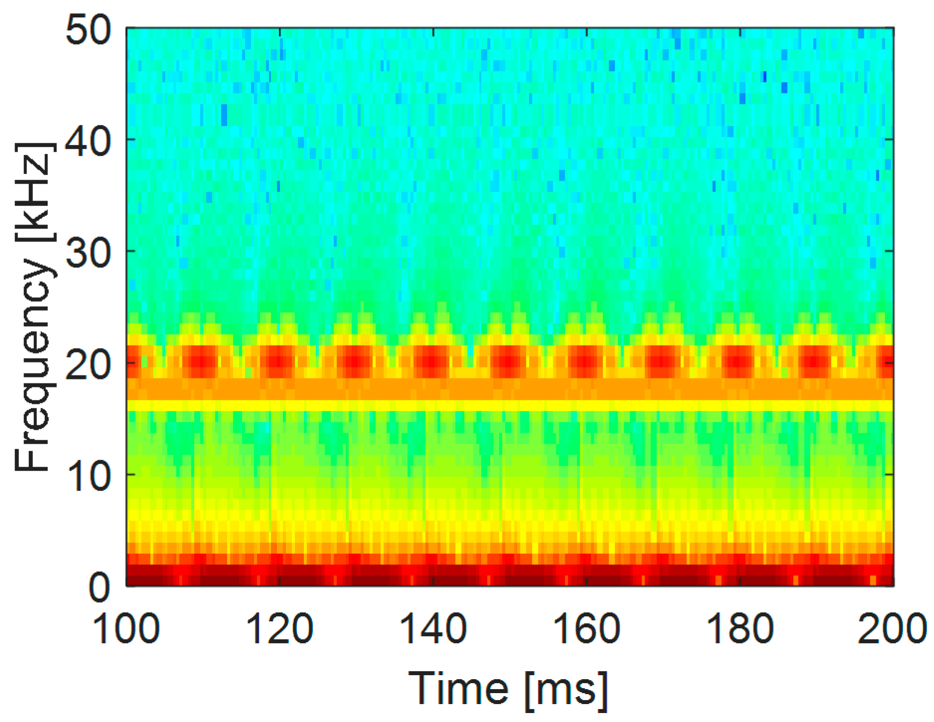
In
Figure 5 the spectrogram with 1 kHz frequency resolution and 1 ms time resolution is shown for the considered waveform, in order to underline the different approach of the spectrogram to the spectral analysis of wide-spectra waveforms in respect to SWWMEM.
As shown in
Figure 5, the spectrogram was able to detect the spectral content both at low-and high-frequency with reduced computational effort, even if a great spread of colour intensity around the real spectral components can be observed, cause of the spectral leakage and of the too large frequency resolution. In particular, the high-frequency spectral components related to the switching frequency appear concentrated around 20 kHz, but, unlike the proposed method, it is impossible to individuate both the correct number of spectral components included in that range and each specific frequency and/or amplitude. Moreover, also a fake periodical variability in time seems to be introduced by this spectral analysis method. Similar behaviour can be observed at low-frequency.
Finally,
Table 2 shows the computational times required by all of the methods to analyze the 3 s waveform, per unit of computational time required by STFTM. It is evident that SWWMEM requires a computational time comparable to that required by STFTM and that SWEM requires a computational time that is about 22 times greater than SWWMEM, providing however results that are globally affected by similar errors. This is due to the presence of the DWT decomposition and of the resampling in the proposed method. In fact, they allow to model both the low-frequency and high-frequency waveforms with a reduced number of exponentials and with a reduced number of samples per analysis window than the SWEM. In this way, the computational burden of the SWWMEM is low although the method holds the accuracy of a parametric method.
4.2. Case Study 2
In this case study, a frequency-modulated, high-frequency spectral component was added to the synthetic waveform of the previous case study. This was made in order to both emulate the presence of secondary emission and to test the performance of the proposed method in the detection of time-varying spectral components, that are typical in the high-frequency range. The added spectral component
was a tone at
with a sinusoidal modulation in frequency, according to Equation (6):
where:
and
was fixed equal to the 0.5% of the fundamental amplitude,
was 5 Hz and
was 1 Hz. The spectral analyses of this waveform were performed through the same settings of the previous case study.
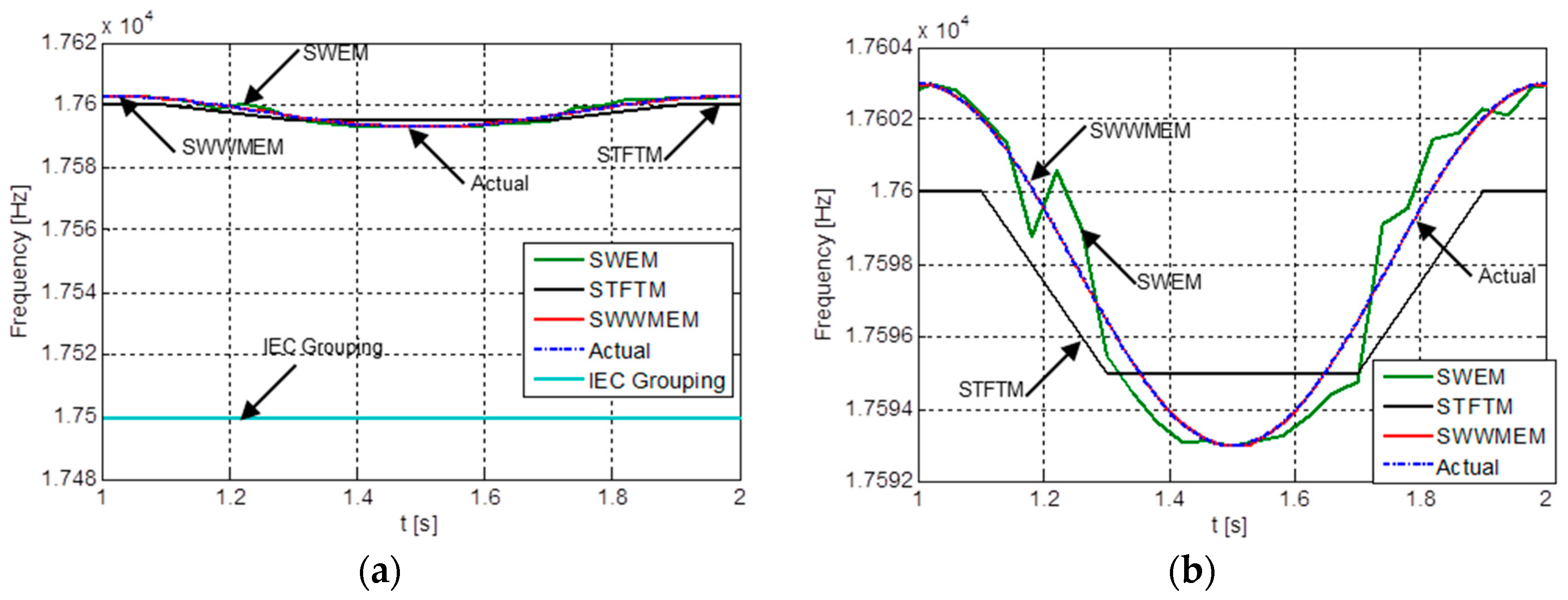
Figure 6 shows few ms of the actual modulated frequency and its estimations obtained through STFTM, SWEM, SWWMEM and IEC grouping. Specifically,
Figure 6a shows that the IEC grouping associates the main part of the energetic content in correspondence of the group at 17.5 kHz.
Figure 6b shows a focus on the graphical comparison among the actual modulated frequency, the STFTM, SWEM and SWWMEM estimations. Note that, since in this case the actual value of the spectral component was known “a priori”, for STFTM it is assumed that a single component is around 17,598 Hz and the other components are spectral leakage. So the modulated component in
Figure 5 is that with the maximum amplitude value in a range of 20 Hz around the actual mean value
. Still, it is clear that STFTM fails the detection due to both the spectral leakage problems and the fixed frequency resolution, while SWEM and SWWMEM are able to clearly identify the modulation. However, the proposed method seemed to provide the best results for this estimation.
Since the average percentage errors on the estimation of the
Table 1 spectral components slightly varied with respect to the results in case study 1,
Table 3 shows only the average percentage frequency errors and the average percentage amplitude errors for the added spectral component. The results are coherent with the behaviors shown in
Figure 4, since the lowest amplitude and frequency errors were provided by the proposed method. In particular, STFTM and SWEM amplitude errors were two order of magnitude higher than SWWMEM amplitude error. Moreover, the average percentage frequency error provided by SWWMEM was two and three orders of magnitude lower than the SWEM and STFTM frequency errors, respectively.
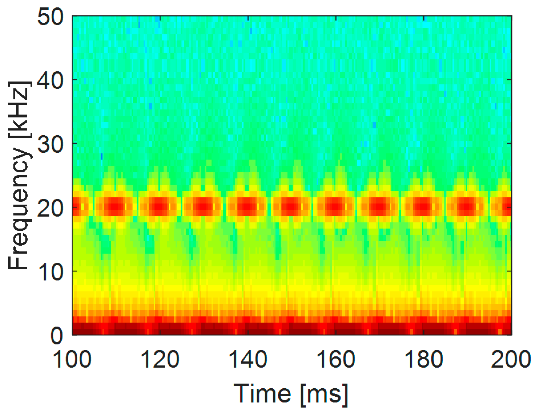
In
Figure 7 the spectrogram with 1 kHz frequency resolution and 1 ms time resolution is shown for the considered waveform, in order to underline once again the different approach of the spectrogram to the spectral analysis of wide-spectra waveforms in respect to SWWMEM.
Similarly to the previous case study, in
Figure 7 the spectrogram was able to detect the presence of spectral content both at low-and high-frequency, but, differently to SWWMEM, only rough and approximated information can be obtained. In particular, also the contribute of the spectral component around 17.958 kHz can be detected, but, in this case the related frequency appears time-invariant, since the real frequency modulation of this spectral component is not individuated, cause of the spectral leakage problems.
Finally,
Table 4 shows the computational time required by the three methods to analyze the 3-s waveform, per unit of computational time required by STFTM. Note that the SWWMEM required a higher computational time than the previous case study, since the frequency variation of the high-frequency modulated component prevented to keep the estimated frequencies constant, requiring often an updating of their value (step 2 of proposed method). However, the time required by SWWMEM was still one order of magnitude lower than the time required by SWEM.
4.3. Case Study 3
A 0.2 s-current waveform measured at the PCC of a single fluorescent lamp powered by high-frequency ballast was analyzed. The total active power consumption of the lamp was about 0.1 kW. The current waveform was measured with a Pearson current probe, model 411. The probe has its 3 dB cut-off frequencies at 1 Hz and 20 MHz with an amplitude accuracy of −0%, +1% in the frequency range of interest. The phase accuracy is less than 1 degree between 60 Hz to 333 kHz. The current was then sampled with 12 bits resolution and 10 MS/s sampling speed, and a low-pass filter with a cut-off frequency 1 MHz was used for anti-aliasing purpose. More details on the installation structure, instrument specification and error verification of measurement are available in [
8,
36].
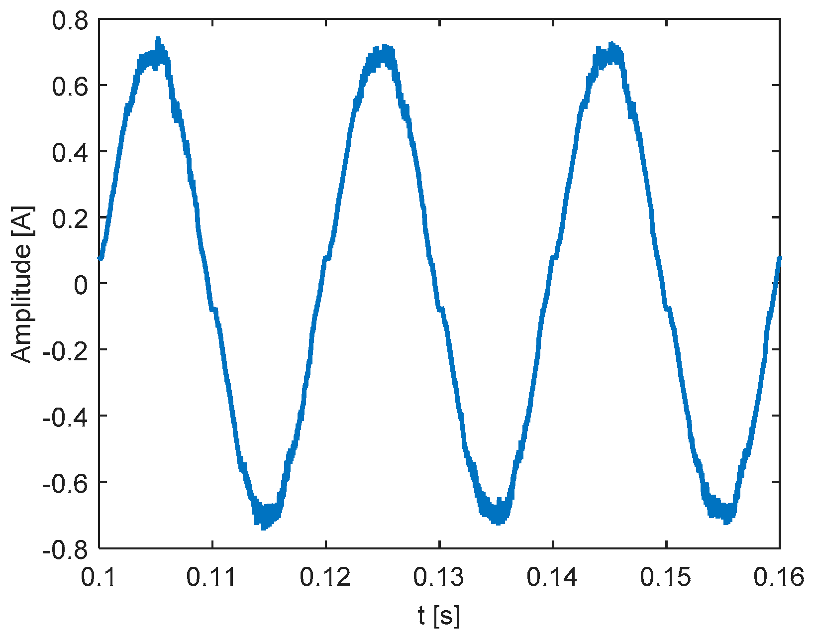
The analyzed current is shown in
Figure 8; the high-frequency components on the peak of the waveform are clearly evident, unlike the high-frequency distortion around the zero crossing.
However, according to the measurement procedure, based on 10 MHz sampling rate, the maximum frequency of interest cannot exceed 5 MHz. In this way, fixing the SWWMEM the bands’ separation frequency to 2 kHz, the maximum number of decomposition levels was 11. A resample to 10 kHz was performed for the low-frequency waveform while the high-frequency waveform was downsampled to 250 kHz, since our interest was the detection of the spectral components up to 150 kHz. Then, the two different waveforms, i.e., and , were analyzed with a sliding window of 0.04 s and of 5 × 10⁻⁴ s, fixing an error threshold of 10−4 and 10−3, respectively. The measured current was downsampled to 250 kHz also for the analyses through SWEM and STFTM, in order to guarantee a correct comparison of the methods in terms of computational burden. In particular, for the SWEM, the error threshold was fixed equal to 10−4, and the sliding window duration was fixed to 0.04 s.
The spectra obtained through the SWWMEM and STFTM were almost similar at low-frequency. In fact, SWWMEM and STFTM individuated the same significant spectral components, though STFTM provided lower amplitudes than SWWMEM cause of the high spectral leakage. These low-frequency spectra included a fundamental component with a peak amplitude equal to about 0.7 A, and all of the other odd harmonics, whose amplitudes globally decrease as the harmonic order increases. These harmonic components reached a maximum amplitude equal to 3.6% of the fundamental in correspondence of the third harmonic, as shown in
Figure 9a.
Figure 9a shows the low-frequency spectrum obtained through SWWMEM, in percentage values of the fundamental amplitude. Finally the SWEM detected a reduced number of spectral components at low-frequency than the other two methods. Probably, this was due to a too high duration of the analysis window that shifted most of the detected spectral components to high-frequency.
At high-frequency, the STFTM spectral leakage increased, spreading the spectral content and missing the detection of specific tones. In particular, a distributed spectral content from 50 kHz to 90 kHz was observed. The same high-frequency spectrum was also detected by SWEM. In both the cases, the amplitudes were decreasing from 50 kHz to 90 kHz, with a maximum equal to the 0.1% and 0.3% of the fundamental amplitude for STFTM and SWEM, respectively. Instead, the proposed method, due to the shorter analysis window, provided a high-frequency spectrum with defined single tones, as shown in
Figure 9b.
The spectrum in
Figure 9b is referred to the first 5 × 10
−4 s of the waveform shown in
Figure 8, but it is very interesting to note that in the following analysis windows the SWWMEM provided a periodic shift of the spectral components around 80 kHz, from 35 kHz to 95 kHz. This means that the proposed method is able to detect a time varying high-frequency spectra.
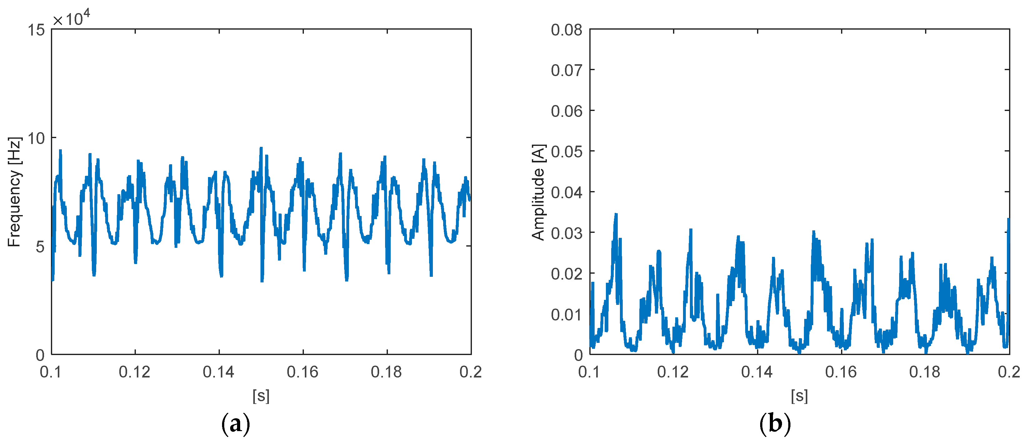
Figure 10 shows the time trend of the spectral component with maximum amplitude detected in the aforesaid range of frequency. Specifically,
Figure 10a shows the frequency variation in time, while
Figure 10b shows the amplitude variation in time. This component could be related to the zero-crossing, since, as shown in
Figure 10, both the frequency and the amplitude variations in time had a periodicity of about 10 ms [
8]. Note also that this component reached the maximum amplitude (about 0.03 A) at about 50 kHz, namely when the positive and negative peaks of the current waveform shown in
Figure 8 occurred.
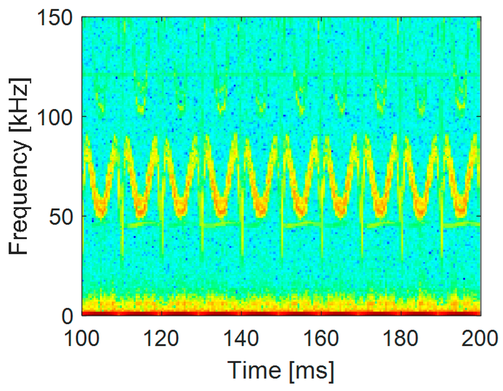
In
Figure 11 the spectrogram with 1 kHz frequency resolution and 1 ms time resolution is shown also for the considered measured waveform, always in order to underline the different approach of the spectrogram to the spectral analysis of wide-spectra waveforms in respect to SWWMEM.
Figure 11 shows the time-varying spectral content in the range from 50 kHz to 100 kHz, so, the spectrogram appeared able to detect significant variations in time of the high-frequency spectral content. However, differently by SWWMEM, once again, only no-detailed information on the specific frequency and amplitude of that spectral component can be obtained.
Finally,
Table 5 shows the computational times required by all of the methods to analyze the waveform, per unit of computational time required by STFTM: the results are coherent to what was theoretically expected, since the computational time required by the proposed method is about four time of that required by ICEM, but it is four order of magnitude lower than that required by the SWEM.
5. Conclusions
In this paper, we proposed a new sliding-window Wavelet-Modified ESPRIT scheme that seems to be particularly suitable for accurate analysis of waveforms that have very wide spectra; the scheme also guarantees a relatively low computational cost.
The method was based on the DWT decomposition of the original signal into low-frequency and high-frequency waveforms, separately analyzed by the SWWMEM in order to provide optimal time and frequency resolutions in each band and, then, an accurate time-frequency representation.
The proposed scheme was tested and evaluated on waveforms measured on an actual power system and on synthetically-generated data sequences, and was compared to the SWEM and the STFTM. These waveforms are characteristic emissions of dispersed generations (such as PVs and WTs) and modern loads (such as fluorescent lamps).
The numerical applications showed that, in presence of slightly time-varying components, the SWWMEM provided almost the same accuracy of the SWEM for both the low-frequency and the high-frequency components with a significantly reduced computational burden. In presence of highly time-varying high-frequency components, instead, the proposed method proved to overcome the limits of both the SWEM and STFTM for the detection of the high-frequency components, still with acceptable computational efforts.
The analyzed case studies give also great emphasis to the inability of the currently available high-frequency signal processing techniques, i.e., the spectrogram with 1 kHz frequency resolution and 1 ms time resolution, in a proper detection of each spectral component included in the wide-spectra (from 0 kHz to 150 kHz) waveforms. The sliding-window Wavelet-Modified ESPRIT scheme provides always detailed information in term of frequency, amplitude and time-variability for both the spectral components at low- and high-frequency.
Based on the aforesaid observations and on the possibility of properly select the duration of the SWWMEM analysis windows, in future works, the proposed method could reveal an adequate tool for the evaluation of new PQ indices in presence of wide spectra. This is due, i.e., to the opportunity of performing a time-aggregation of the spectral components in the range from 2 kHz to 150 kHz, in opposition or complementarily to the currently-proposed frequency-aggregation.


