Thermal Simulation of the Fresh Food Compartment in a Domestic Refrigerator

Abstract

In the field of domestic refrigeration, it is important to look for methods that can be used to simulate, and, thus, improve the thermal behavior of the fresh food compartment. In this sense, this study proposes some methods to model the thermal behavior of this compartment when the shelves’ positions are changed. Temperature measurements at specific locations in this compartment were obtained. Several shelf position combinations were performed to use three 2D interpolation methods in order to simulate the temperature mean and the temperature variance. The methods used were: Lagrange’s interpolation, cubic spline interpolation and bilinear interpolation. Two validation points were chosen to verify the proposed methods. By comparing the experimental results with the computer simulations, it was possible to conclude that the method of Lagrange’s interpolation provided values that were not close to the real measured values. On the other hand, it was observed that the method of bilinear interpolation offered the best results, estimating values which were very close to the actual experimental measurements. These interpolation methods were used to build color thermal graphs that can be used to find some of the most appropriate shelf position combinations in this type of refrigerator. By inspection of these thermal graphs, it can be seen that the lowest average temperature was obtained when one shelf was located at 24.5 cm while the second shelf was located at 29.5 cm measured from the top of the compartment. In the same way, it can be seen that the minimum temperature variance was obtained when only one shelf was inside the compartment and this shelf was located at 29.5 cm.

1. Introduction

The domestic refrigerator is one of the most used appliances worldwide and the majority of these refrigerators are based on the vapor compression technology; thus, in literature, several studies have focused on thermal improvements and energy strategies in the system operation [1,2]. On the other hand, it is known that the basic function of the refrigerator is storing fresh food and medicines, and this depends on the good performance of the refrigerator, which is closely linked to temperature distribution and air flow inside the compartments. Adequate temperature in these refrigerators could significantly extend the living cycle of food [3] and, inclusively, avoid the growth of certain types of bacteria [4]. In addition, the thermal behavior is influenced by the refrigeration system design, while the proper temperature distribution is achieved by a good interior design of the refrigerator.

The temperature and air flow distribution in the compartments (the fresh food compartment and the freezer) have been studied in the literature, where numerical methods and mathematical approaches have been used to predict the temperature distribution inside the refrigerator. For instance, Ding et al. [5] applied the Computational Fluid Dynamics (CFD), reaching the conclusion that temperature distribution depends on the internal geometry of the refrigerator, specifically in the spaces between the refrigerator shelves and the liner bottom wall, as well as on the edge of the shelves and the door. It is concluded that, when reducing both spaces, temperature variation will decrease and more uniform temperature distributions will be reached. Afonso and Matos [6] measured the inside air temperature with and without radiation shield. Additionally, they used the Fluent software to simulate the internal air temperature in both situations. Results showed that when the surfaces are covered with a sheet of aluminum foil, this represents a significant decrease in the inside air temperatures of the fresh food and the freezer compartment (about 2 K). Gupta et al. [7] introduced the development of a model in CFD for a frost-free refrigerator where they predicted and experimentally compared temperature profiles. The authors concluded that the trends in computational and experimental results are qualitatively similar. Additionally, they proposed some modifications in the design to improve the performance of the refrigerator. Yang et al. [8], through simulations, proposed a new design of the shelves in the air outlets, achieving a better thermal profile with a reduction of temperature from 7.17 to 3.57 ${}^{\circ }$C in the refrigerating compartment. Torabi et al. [9] worked particularly in the freezer of a natural convection refrigerator, by means of experimentation and the use of CFD. They analyzed the design of seventeen models to optimize the field of temperatures in the freezer. As a result of this optimization, a better distribution of the air flow and heat transfer in the freezer is obtained. Björk et al. [10] used a thermographic camera to observe the temperature distribution of a domestic refrigerator as an alternative method to analyze the cooling system. Their study reveals sources of energy losses that would have been difficult to find if the conventional temperature measurement technique (i.e., thermocouples) had been used. Laguerre and Flick [11] presented some deterministic and stochastic approaches to predict the air and temperature in a static refrigerator. Their model allows the calculation of temperatures at the top and at the bottom of the cavity, and it can be linked to a predictive microbiological model to estimate the probability of contamination. Kumlutas et al. [12] developed an artificial neural network model and applied numerical simulations to find the temperature distribution inside a static type refrigerator in order to predict the design parameters as: gap between evaporator surface and glass shelf, evaporator height and surface temperature. Consequently, their model is a successful method for the designers to obtain a preliminary assessment for design parameter modifications in static refrigerators. Bayer et al. [13] simulated the fluid flow with a reduced order modeling method and analyzed the temperature distribution in a refrigerator compartment. Thus, taking radiation effects into consideration does not change the temperature distribution inside the refrigerator significantly. However, the heat rates are affected drastically. Belman-Flores et al. [14] analyzed the thermal stratification in the compartments of a forced convection refrigerator through CFD, and their results were experimentally validated. The geometric proposal was experimentally compared with the original configuration, resulting in a diminishing of the average temperature in the fresh food compartment. They found better thermal profiles with the proposal of a new interior design.

Based on the above, it can be said that some researchers have experimentally analyzed the temperature distribution in the compartments, while other researches have analyzed this temperature distribution through the use of CFD, and some others have used mathematical methods to simulate and compare the thermal behavior of the fresh food compartment. Thus, it is clear that these methods to improve the temperature uniformity inside domestic refrigerators are still an open area for more research. In this context, it can be said that the temperature distribution is directly influenced by: the geometric configuration, the accessories’ positions in the compartment and the internal volume. Therefore, this study was carried out in order to continue and extend previous works that use mathematical approaches to simulate the thermal behavior of the compartments in a domestic refrigerator.

In this paper, a test refrigeration facility was setup in order to analyze the thermal performance of a refrigerator. Thus, a set of thermocouples was installed inside the refrigerator to monitor the thermal distribution for several shelves’ locations in the fresh food compartment. Three interpolation methods are considered to simulate the thermal behavior in the fresh food compartment. These methods are used to perform computer simulations in order to build 2D color graphs to show the effect of the shelves’ locations on the temperature. Some of these graphs indicate the mean temperature in the fresh food compartment, while other graphs are used to illustrate the thermal dispersion in this compartment. The main contribution of this work is the application of these graphs that offer an opportunity to incorporate thermal improvements in this type of domestic refrigerator.

Techniques for Designing the Fresh Food Compartment

As it was previously explained, the thermal conditions of the storage of food products depend on an appropriated temperature distribution inside the refrigerator compartments. This without forgetting a correct design of the vapor compression cycle. Furthermore, the compartments temperature is also related to the internal design of the refrigerator. In most cases, the interior of a refrigerator may be innovative. However, it must be designed so that it has plenty of space. In the same way, the illumination system in combination with transparent shelves make the perception of the interior space bigger than it is. This space, however, is manipulated by the position of the shelves.

In the last few decades, the lifestyles of different societies have produced an increase in the size of the freezer as well as in the size of the fresh food compartment. These compartments may have different characteristics according to the refrigerator type (double door, top mount, bottom mount, etc.), influencing its internal volume and its thermal behavior. In this sense, the design of the compartments is related to their capacity, thus taking into consideration the requirements for most applications. For instance, the fresh food compartment is the biggest in a domestic refrigerator. In this compartment, food must be kept at 3 ${}^{\circ }$C in most refrigerators when the damper position is 5 (see [1]). This compartment is usually divided by the shelves in order to make the food organization easy for the user.

2. Experimental Analysis

In order to analyze the thermal performance, experimental tests were conducted. The domestic refrigerator used for the simulations has a total volumetric capacity of 0.28 m${}^3$ (10 ft${}^3$). Other characteristics of this refrigerator are included in

Table 1. General characteristics of the refrigerator.

Name	Value
Net weight	47 kg
Total depth	65.5 cm
Total height	169 cm
Total width	61.8 cm
Defrost	Automatic
Refrigerant	R134a
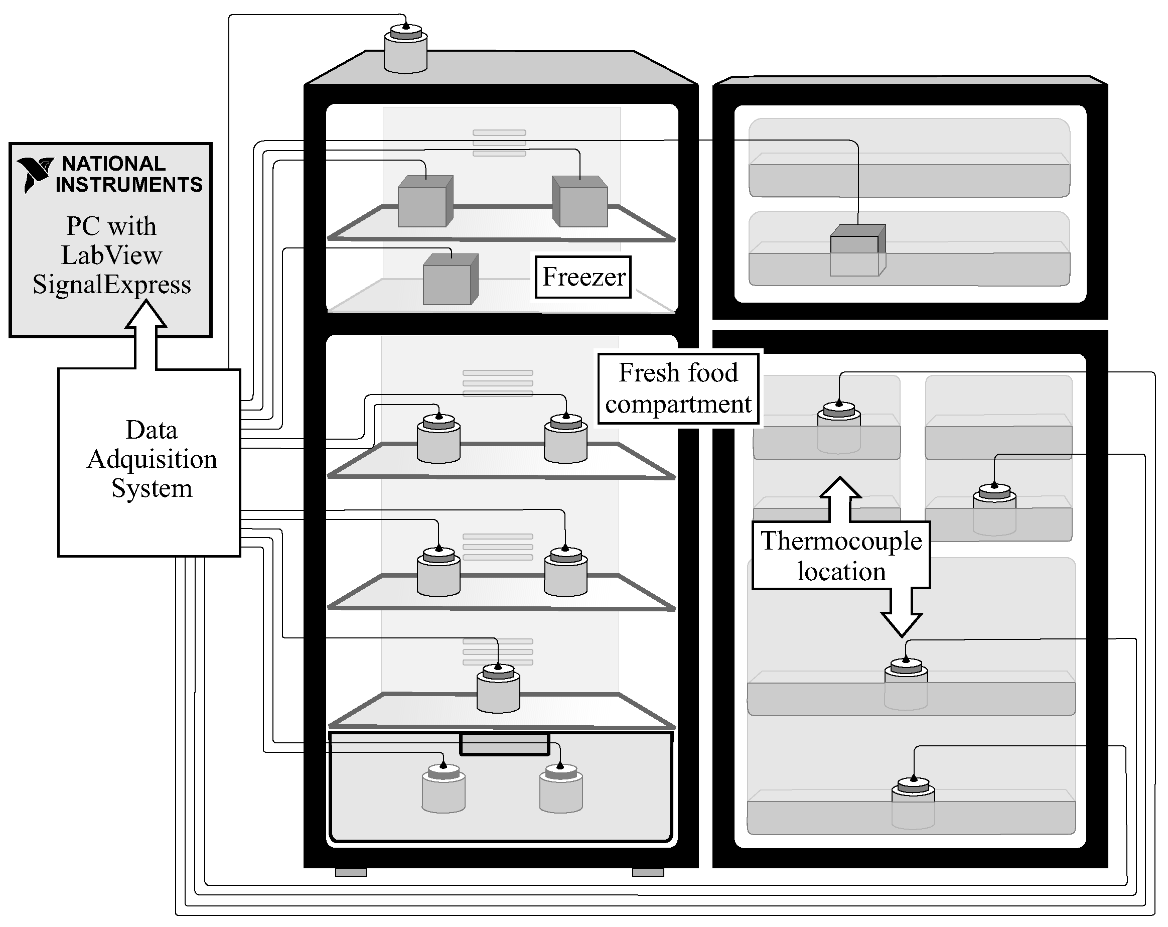
Configuration	Top mount, two doors

. The experimental refrigerator has two main compartments: the fresh food compartment and the freezer; the refrigerator scheme is shown in Figure 1. In this no-frost refrigerator, the heat transfer is mainly done by forced-convection since the air flow is propelled by a fan (with a volumetric flow of 0.028 m${}^3$/s) located in front of the evaporator inside the freezer, with a position of 0.45 inches. During all tests in this work, the refrigerator doors remained closed until thermal stability was reached in the compartments. Consequently, the relative humidity of the air that produces the accumulation of frost was not considered in this study. Additionally, during test periods, no defrost operations were performed in the refrigerator.

The fresh food compartment has two solid glass shelves that can be adjusted according to the volume of the food supplies. Therefore, it is possible to arrange them at several fixed positions. The effect of the spacing between the shelves on the thermal distribution of the refrigerator is the main topic of this work. Finally, it can be noted that the freezer has only one solid glass shelf.

Instrumentation and Measurements

The refrigerator under study was instrumented in order to measure temperature in several parts of the compartments. For instance, in the fresh food compartment, 11 thermocouples were placed inside containers of $0.2451$ (0.000245 m${}^3$) with a mixture of 50% in volume of water and glycol. These containers were distributed on: the glass shelves, the vegetable drawer and the door shelves (see Figure 1). On the other hand, temperature measurements in the freezer were obtained using four thermocouples placed inside wooden blocks in order to avoid density changes as well as volume changes during the test. The blocks were distributed in the compartment. This type of instrumentation is according to the methodology recommended by this specific refrigerator manufacturer. Note that temperature sensors were calibrated in our laboratory using certified references, and the obtained temperature uncertainty was $\pm 0.3$ K.

Several tests were performed with a duration of approximately 9 h. These tests included the transitory behavior during the startup and the halt of the compressor. The refrigerator operated at a constant room temperature of 294 ± 1.5 K and with a relative humidity of 60% ± 5%. The signals generated by the sensors were stored through a NI-9213 data acquisition card from National Instruments, Subsequently, the system was connected via USB port to a computer that allowed monitoring the equipment’s experimental conditions in real-time through the use of the SignalExpress 2015 software, which was programmed in LabView 2015. Note that temperature measurements were taken at intervals of 10 s.

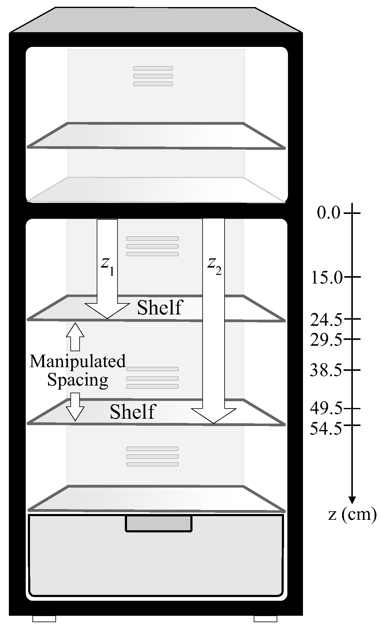
The tests in this work involved the manipulation of the spacing between the shelves (see Figure 2) in order to analyze and simulate its influence over the thermal behavior of the refrigerator compartments. In this figure, $z_1$ indicates the distance from the first shelf to the upper part of the compartment, while $z_2$ represents the distance from the other shelf to the same reference point. For this work, 22 fixed positions (tests) were chosen so that the minimum space allowed the use of the compartments without blocking the air outlets.

Table 2. Shelf configurations.

Shelf 1	Shelf 2	Temperature	Temperature
Location: ${\mathit{z}}_1$ (cm)	Location: ${\mathit{z}}_2$ (cm)	Mean ${}^{\circ }$C	Variance (${}^{\circ }$C)${}^2$
0	0	4.25	1.82
15	15	4.52	1.62
15	24.5	4.84	1.97
15	29.5	4.60	1.54
15	38.5	4.92	1.89
15	49.5	5.43	4.64
15	54.5	4.61	2.96
24.5	24.5	4.82	1.83
24.5	29.5	3.31	2.76
24.5	38.5	4.78	1.85
24.5	49.5	4.64	2.41
24.5	54.5	3.55	2.76
29.5	29.5	4.45	0.99
29.5	38.5	3.70	3.49
29.5	49.5	3.48	4.44
29.5	54.5	4.55	3.06
38.5	38.5	4.28	3.65
38.5	49.5	4.30	5.15
38.5	54.5	4.91	4.80
49.5	49.5	4.29	4.83
49.5	54.5	4.51	2.36
54.5	54.5	4.37	2.23

indicates the shelf configurations used in this work, the table also includes the temperature mean and the temperature variance for each configuration. The thermal color graphs, described later, provide a visual method to understand the effect of the shelf configuration on the temperature mean and the temperature variance. Each test began at the same temperature condition (21 ${}^{\circ }$C), and ended approximately 9 h later once the thermal stability was reached.

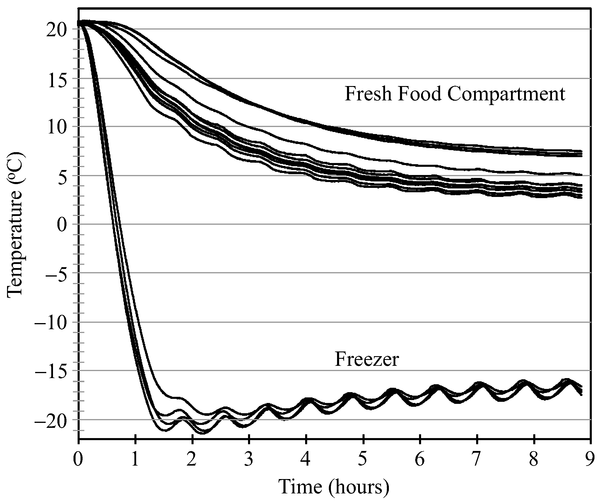
Thus, Figure 3 shows the thermal profile for both compartments using the shelf position and the damper position 5, as it is shipped out factory. In this figure, it can be appreciated that the fresh food compartment shows temperatures in an approximate range from 3 to 8 ${}^{\circ }$C once thermal stability has been reached. On the contrary, the freezer temperature goes from $-18$ to $-16{}^{\circ }$C. Thus, it can be seen that the refrigerator presents greater thermal variability in the fresh food compartment than in the freezer. This is the main reason why this study focuses on the analysis of the fresh food compartment.

At the beginning of each test, the compressor is ON for a long time, approximately 1 h and 20 min; after this period, the compressor is OFF for a very short period of time in a constant manner. At the beginning of the test, the thermal condition in the freezer is very low and, due to the thermal calibration condition between both compartments and the rate between the ON–OFF periods of the compressor, the temperature in the freezer slowly increases until thermal stability is reached in both compartments, as it can be observed in Figure 3.

3. Unidimensional Interpolation

In this section, the general concept of interpolating the value of a function $f\left(x\right)$ for a specific x will be explained. Thus, this section provides background knowledge to understand multidimensional interpolation that is necessary for this study. In the field of applied engineering, given a set of data samples $f\left(x_1\right),f\left(x_2\right),...,f\left(x_N\right)$ obtained typically by experimentation, it is sometimes necessary to estimate the value of $f\left(x\right)$ for an arbitrary x that is between the smallest and the largest value in the set of points $x_1,x_2,...,x_N$, [15]. This process of estimating $f\left(x\right)$ in this range of values is called interpolation.

The process of interpolation may be accomplished by curve fitting or regression analysis, and it typically requires a functional form that typically uses polynomials, rational functions or trigonometric functions. This functional form must be as general as possible in order to be able to approximate a wide set of functions that might happen in real-life applications [15]. From a practical point of view, linear interpolation, Lagrange’s interpolation or cubic spline interpolation may be used in this study.

3.1. Lagrange’s Interpolation

It is possible to compute an interpolating polynomial of degree $N-1$ using Lagrange’s interporlation

$$\begin{array}{cc}\hfill P\left(x\right)=& \frac{(x-x_1)(x-x_2)\cdots (x-x_{N-1})}{(x_0-x_1)(x_0-x_2)\cdots (x_0-x_{N-1})}f\left(x_0\right)\hfill \\ & +\frac{(x-x_0)(x-x_2)\cdots (x-x_{N-1})}{(x_1-x_0)(x_1-x_2)\cdots (x_1-x_{N-1})}f\left(x_1\right)+\cdots \hfill \\ & +\frac{(x-x_0)(x-x_1)\cdots (x-x_{N-2})}{(x_{N-1}-x_0)(x_{N-1}-x_1)\cdots (x_{N-1}-x_{N-2})}f\left(x_{N-1}\right).\hfill \end{array}$$

(1)

There are several advantages of Lagrange’s formula. However, it does not provide an estimate of the interpolation error. Thus, Neville’s algorithm is preferred for some applications. Neville’s algorithm is used for polynomial interpolation using the following recursion equations:

$$P_{i,i}\left(x\right)=f\left(x_i\right),0\le i\le N-1,$$

(2)

$$P_{i,j}\left(x\right)=\frac{(x_j-x)P_{i,j-1}\left(x\right)+(x-x_i)P_{i+1,j}\left(x\right)}{x_j-x_i},0\le i\le j\le N-1.$$

(3)

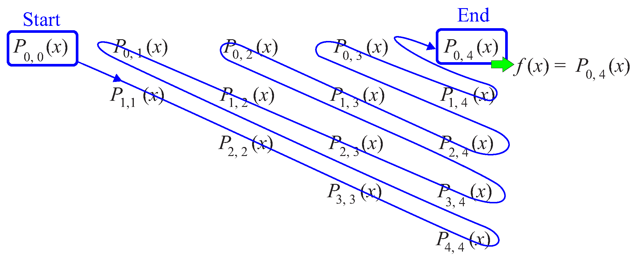
In the last equation, $P_{i,j}\left(x\right)$ denotes a polynomial of degree $j-i$. Neville’s algorithm provides an iterative method to perform interpolation. However, Neville’s algorithm may be difficult to understand, and it is commonly explained using a step by step diagram. Figure 4 illustrates how this algorithm is evaluated when N is four. The algorithm begins by computing: $P_{0,0}\left(x\right)$, $P_{1,1}\left(x\right)$, $P_{2,2}\left(x\right)$, $P_{3,3}\left(x\right)$, $P_{4,4}\left(x\right)$. Then, Equation (3) is used to compute $P_{0,1}\left(x\right)$. The algorithm continues the recursion until the desired interpolated value is found; in this case $P_{0,4}\left(x\right)$ (see [15]). An easy way to understand the diagram in Figure 4 is observing that each $P_{i,j}\left(x\right)$ represents a numeric value in a table, and the P is used to indicate polynomial. The figure only illustrates how these numeric values are computed by using Equation (2). The last value in the algorithm is the required interpolated value.

3.2. Cubic Spline Interpolation

This type of interpolation uses a set of cubic splines to perform the interpolation. The goal of cubic spline interpolation is to get an interpolation formula that is smooth in the first derivative, and continuous in the second derivative, both within an interval and its boundaries [15]. In numerical analysis, spline interpolation is frequently preferred over polynomial interpolation because the interpolation error is small even when third degree polynomials are used. For some applications, small degree polynomials may interpolate better than high degree polynomials. In fact, linear interpolation may provide satisfactory results in some special cases.

4. Multidimensional Interpolation

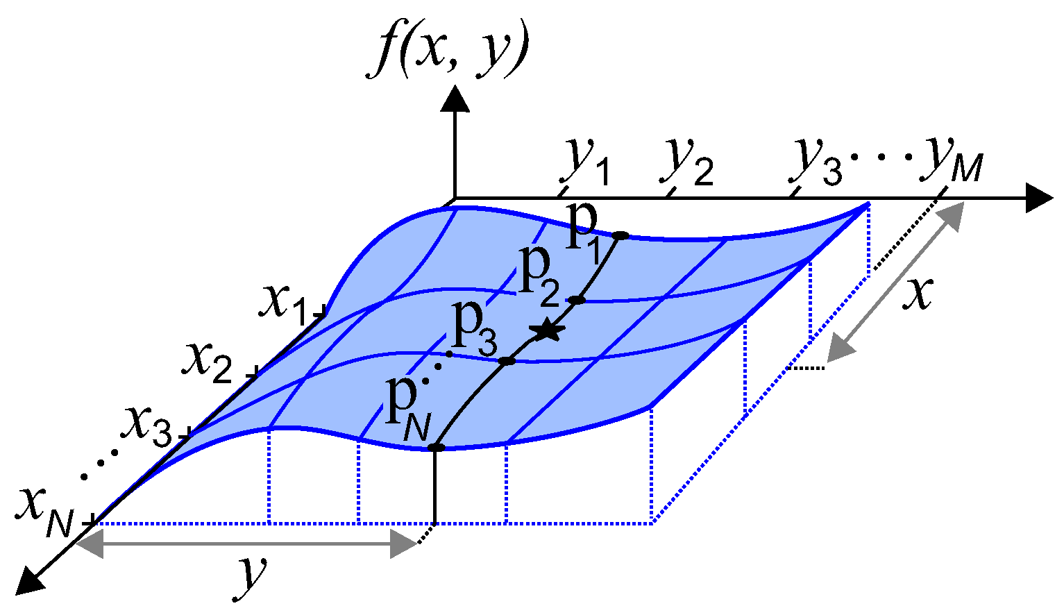
In multidimensional interpolation, the desired estimate is computed from an n-dimensional grid of tabulated values. Figure 5 shows how two-dimensional interpolation is performed. In this case, there are two sets of values: $x_1$, $x_2$, $x_3$, ⋯, $x_N$ and $y_1$, $y_2$, $y_3$, ⋯, $y_M$. Thus, given another set of values $f(x,y)$ for each point in this two-dimensional grid, it is desired to estimate $f(x,y)$ for any arbitrary x and y with $x_1\le x\le x_N$ and $y_1\le y\le y_M$. In this figure, the star represents the point where it is desired to perform the interpolation.

Interpolation in two dimensions can be accomplished by using a sequence of unidimensional interpolations as it is described next. First, the value of $p_1$ is estimated using the values of $f(x_1,y_1)$, $f(x_1,y_2)$, ⋯, $f(x_1,y_M)$. Second, the value of $p_2$ is estimated using the values of $f(x_2,y_1)$, $f(x_2,y_2)$, ⋯, $f(x_2,y_M)$. The process continues until all values of p have been computed using unidimensional interpolations. Finally, the desired value of $f(x,y)$ is estimated from $p_1$, $p_2$, ⋯, $p_N$ using another unidimensional interpolation. Applying this procedure, it is possible to use Lagrange’s interpolation and cubic spline interpolation to estimate a value from a grid of values in two dimensions.

Another easy method to perform two-dimensional interpolation is called bilinear interpolation. In this method, the interpolation is performed by interpolating the four points that are next to the point where it is desired to interpolate. For some applications, bilinear interpolation is frequently very good. Despite the fact that the interpolated function changes continuously, the gradient of the interpolated function changes discontinuously at the boundaries of each grid squared (see [15]).

For this work, 2D interpolation was used to compute the average temperature and the temperature variability as a function of the shelf positions. Thus, in this specific case, $z_1$ and $z_2$ are the input variables for the interpolation algorithm. Therefore, the output of the interpolation algorithm is the temperature average (and the temperature variability) for any values combination of $z_1$ and $z_2$.

5. Computer Simulations and Results

In this section, several computer simulations using the C++ language are performed. First, the mean temperature in the fresh food compartment is analyzed. Second, the thermal homogeneity in this compartment is computed. Thus, three interpolation methods are discussed in both cases, and the respective results are analyzed.

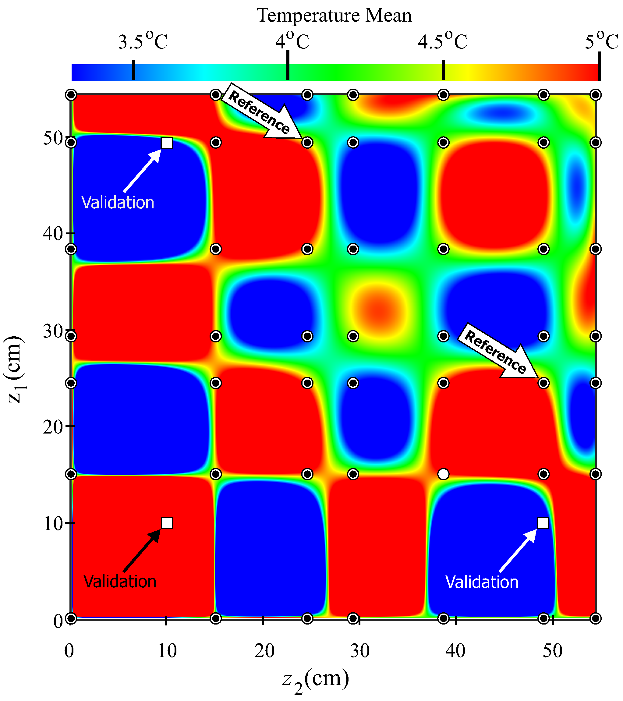
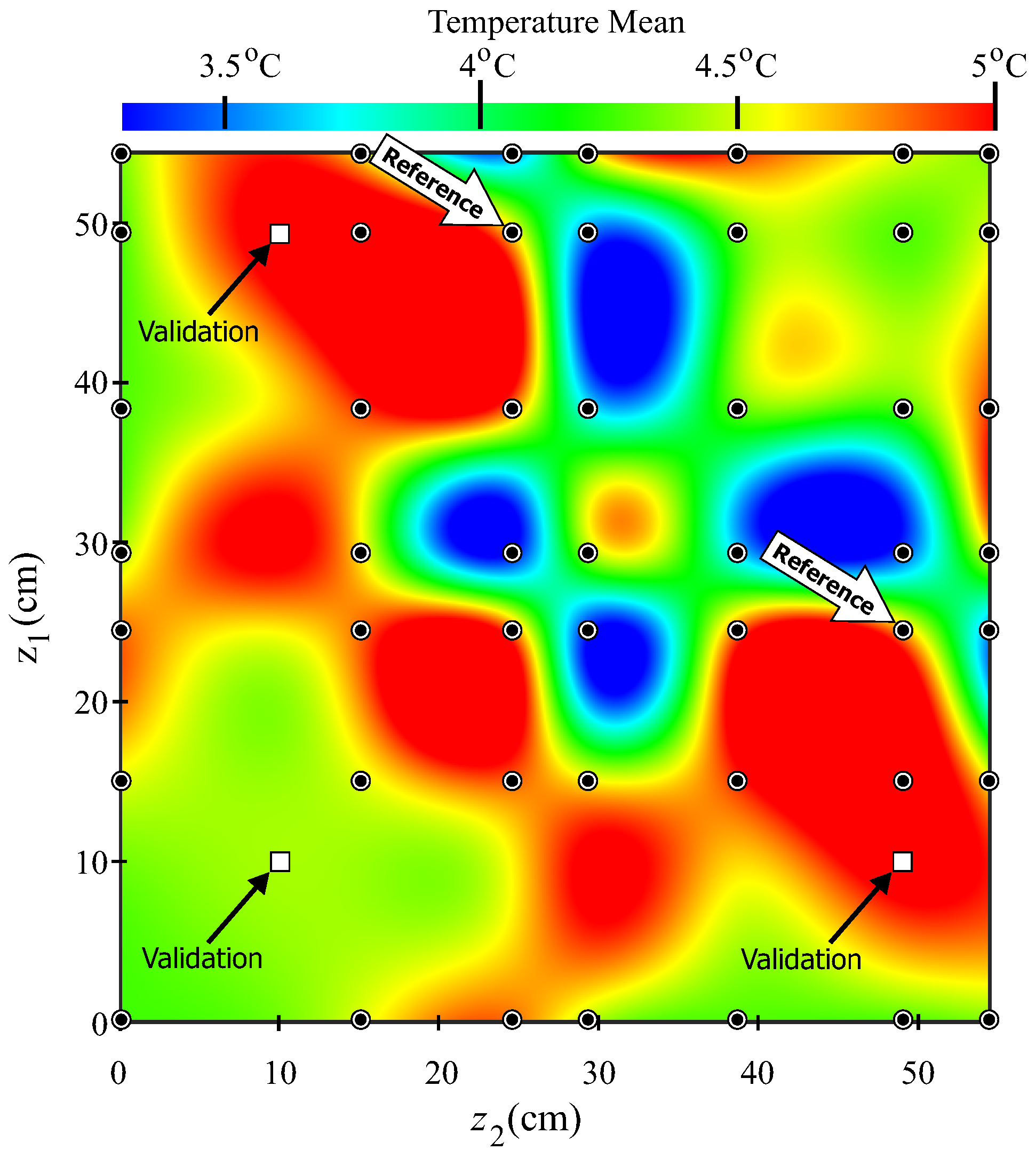
5.1. Temperature Mean

Figure 6 shows the thermal simulation for Lagrange’s formula (see Equation (1)). In this figure, the mean temperature as a function of the shelf positions is shown; note that the mean temperature is the average of all sensors in the fresh food compartment. The mean temperature is displayed by a color scale, the blue color represents low temperatures (around 3.5 ${}^{\circ }$C), while red is used to indicate high temperatures (around 5 ${}^{\circ }$C). On the other hand, the small black circles are used to indicate the average temperature for the experimental tests. The arrows indicate the reference point, that is, the average temperature where the shelves are located as the refrigerator is shipped out of factory. Note that the reference point is displayed twice because of the map symmetry.

The point indicated by the white circle (in Figure 6) is used to explain how the manipulating space was adjusted for the simulation. Thus, the white point has $z_1=15$ cm. This implies that shelf 1 is located at 15 cm measured from the internal upper part of this compartment (see Figure 2), while $z_2=38.5$ cm implies that the other shelf is located at $38.5$ cm from the same reference. The color red, in this case, indicates a temperature of around 5 ${}^{\circ }$C. Thus, this figure indicates the average temperature when the position of the shelves change (that is, when $z_1$ and $z_2$ change).

In order to validate the application (thermal simulation) of Lagrange’s interpolation, two validation shelves combination were chosen. These two points are marked by white squares in Figure 6: validation 1 and validation 2. validation 1 is performed with $z_1=10$ cm and $z_2=10$ cm, implying that there is only one shelf inside the fresh food compartment. For this case, the experimental mean temperature was 4.44 ${}^{\circ }$C; however, the method of Lagrange’s interpolation estimated a value of 5 ${}^{\circ }$C. The other validation point, validation 2, was performed with $z_1=10$ cm and $z_2=49.5$ cm. In this case, the experimental mean temperature 4.95 ${}^{\circ }$C, while the estimated temperature using Lagrange’s method was 3.25 ${}^{\circ }$C. One important aspect to notice in this type of interpolation is that the temperature abruptly changes when the shelves are slightly moved.

Figure 7 shows the validation results for the method of cubic splines. For validation 1, the experimental mean temperature was 4.44 ${}^{\circ }$C while the interpolated value was 4.4 ${}^{\circ }$C. With respect to validation 2, the experimental mean temperature was 4.95 ${}^{\circ }$C, while the estimated value was 4.95 ${}^{\circ }$C. As it can be seen, the method of cubic spline provides better approximated values than Lagrange’s method. Finally, Figure 8 displays the thermal simulation for the bilinear interpolation method. In this case, the estimated value for validation 1 was 4.5 ${}^{\circ }$C and 4.95 ${}^{\circ }$C for validation 2 was. After comparing the interpolated values using the three methods, it can be observed that the method of cubic spline provides the best results. However, the method of bilinear interpolation also provides good results. On the other hand, the abrupt thermal changes presented in Lagrange’s method indicate that this method is not suitable to simulate the thermal performance of the fresh food compartment.

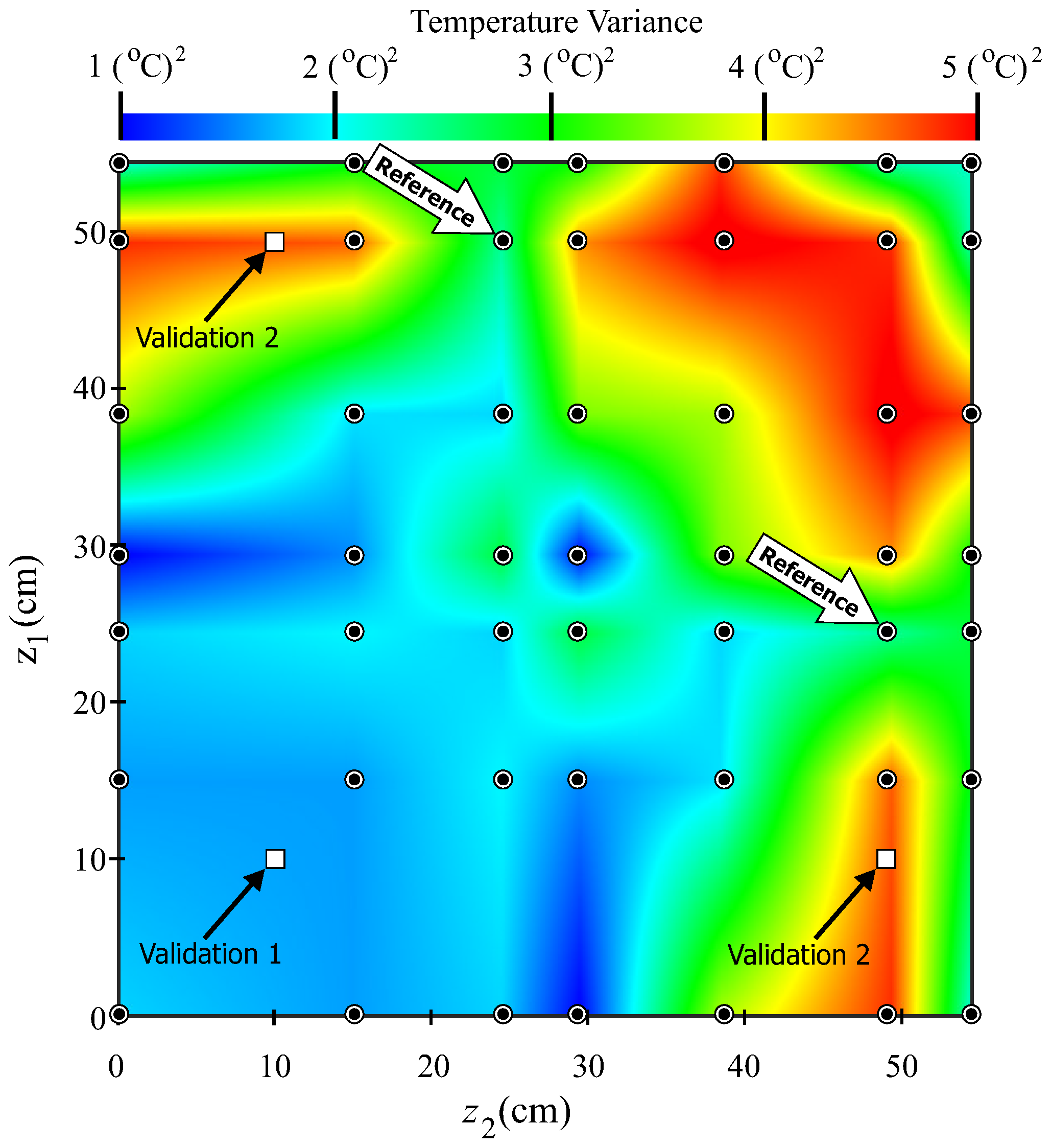
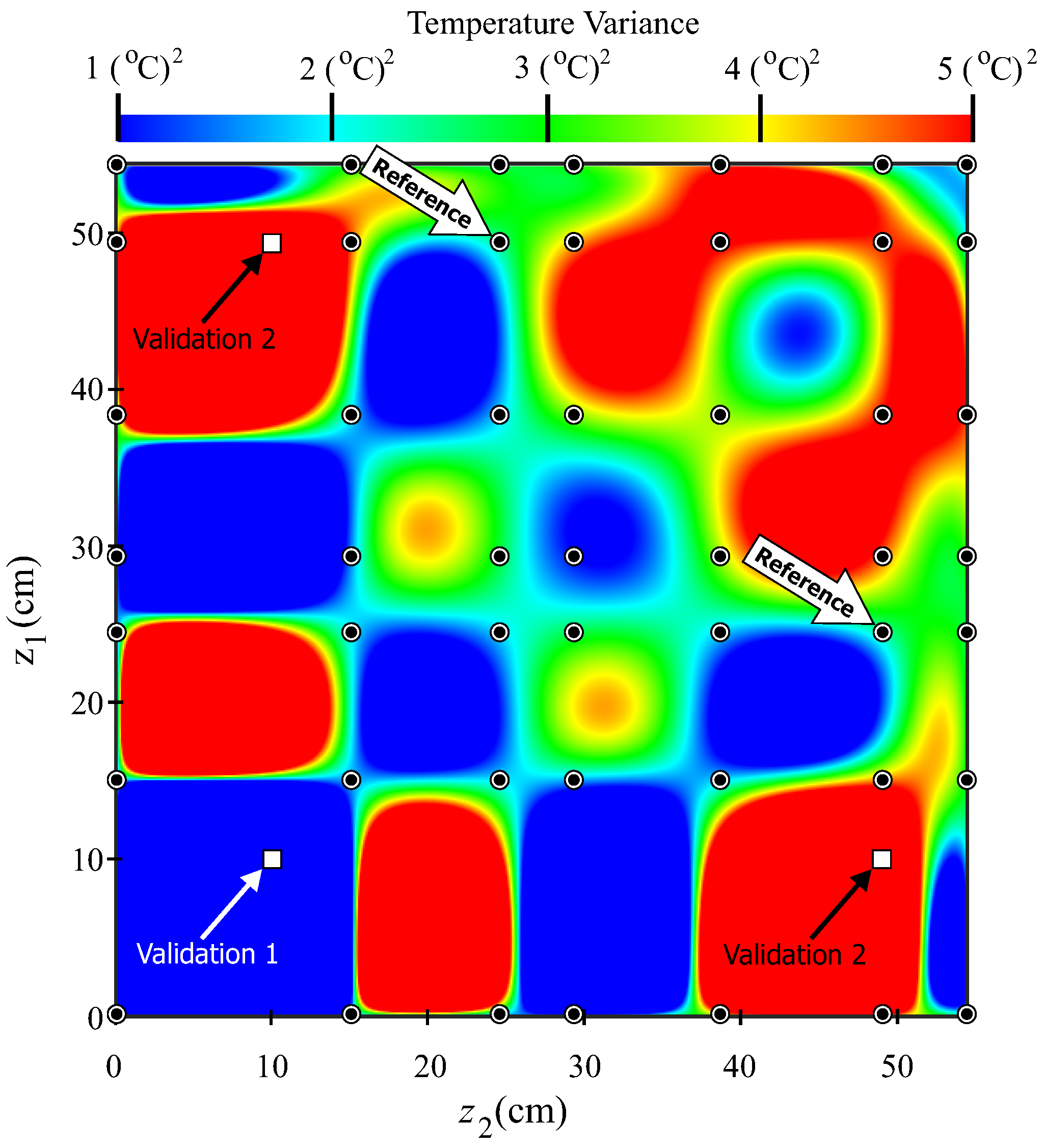
5.2. Temperature Variance

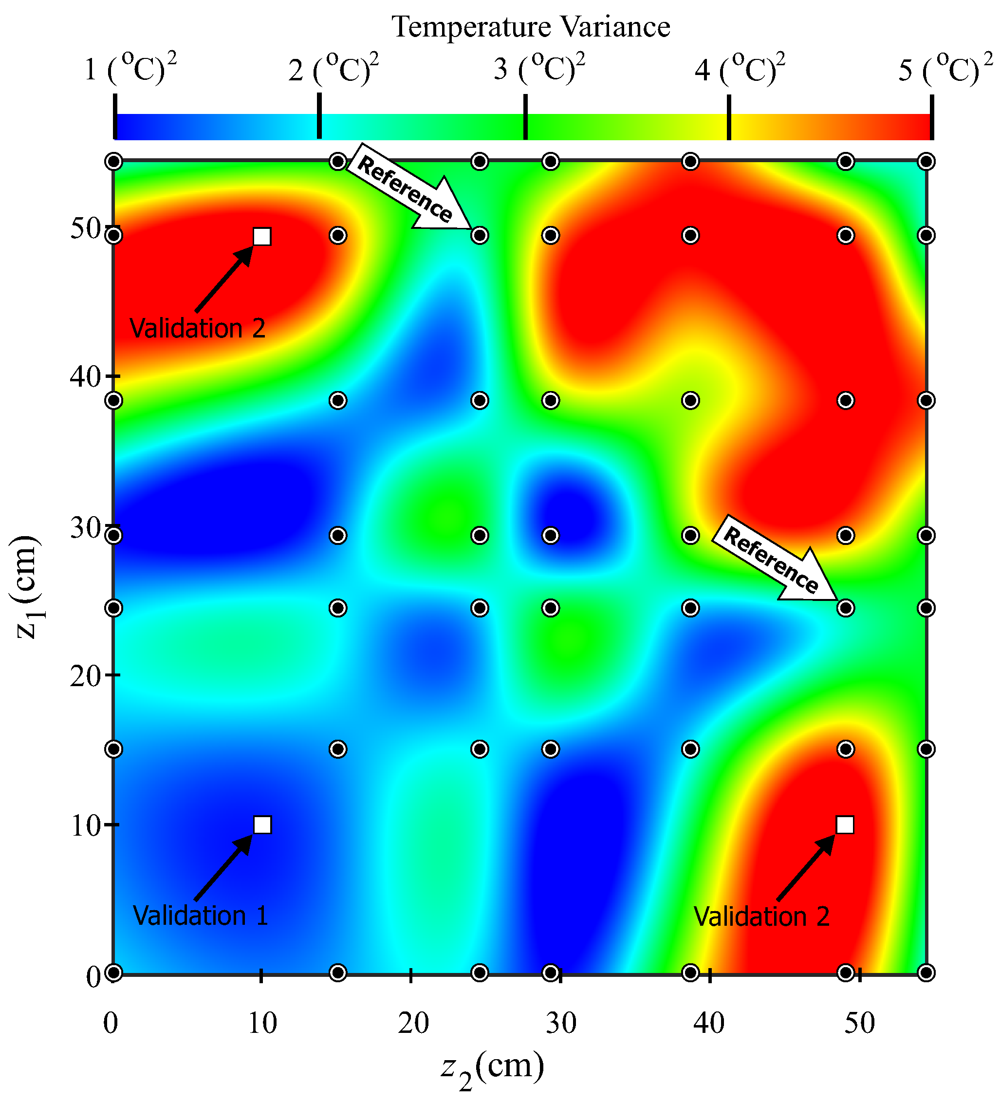
Figure 9, Figure 10 and Figure 11 depict the temperature variance computed among all sensors (thermocouples) in the fresh food compartment. Because, in the area of domestic refrigeration, it is essential to reduce thermal variations in different zones in the fresh food compartment, these figures illustrate the simulation of the temperature homogeneity as a function of the shelf position. In these figures, the temperature variances is displayed using several colors. Specifically, a blue color represents the lowest variance—in this case 1 (${}^{\circ }$C)${}^2$. The zones with highest variability are displayed in red—in this case 5 (${}^{\circ }$C)${}^2$. Additionally, these figures also exhibit the actual experimental tests and the reference position. In this case, the thermal variation at the reference (with the shelves located as shipped out of factory) is 2.4 (${}^{\circ }$C)${}^2$, as it can be observed from the figures.

Figure 9 shows the temperature variance simulation using Lagrange’s interpolation. For validation 1, the experimental temperature variance was 1.67 (${}^{\circ }$C)${}^2$ while the interpolated value was 1.0 (${}^{\circ }$C)${}^2$. With respect to validation 2, the experimental temperature variance was 4.7 (${}^{\circ }$C)${}^2$ while the estimated value was 5.0 (${}^{\circ }$C)${}^2$.

Figure 10 shows the simulation for the temperature variance using the method of cubic splines. For this case, the estimated variance was 1.4 (${}^{\circ }$C)${}^2$ for validation 1, while the thermal variance for validation 2 was 5.0 (${}^{\circ }$C)${}^2$ .

Finally, Figure 11 displays the results for the bilinear interpolation method. Here, the estimated variance was 1.7 (${}^{\circ }$C)${}^2$ for validation 1, while the thermal variance for validation 2 was 4.7 (${}^{\circ }$C)${}^2$. By comparing Figure 9, Figure 10 and Figure 11, it can be seen that the method of Lagrange’s interpolation presents very abrupt color changes, while the method of bilinear interpolation exhibits very smooth color transitions. Because, in practice, large thermal variations are not expected when shelves are changed to different positions, it can be concluded that the method of Lagrange’s interpolation does not represent the actual behavior of the refrigerator.

After presenting the thermal simulations for the three methods, we proceed to compare the validation results for the temperature mean and temperature variance. The experimental measured values are displayed in the first row of

Table 3. Method comparison.

Interpolation	Validation 1		Validation 2
	Mean ${}^{\circ }$C	Variance (${}^{\circ }$C)${}^2$	Mean ${}^{\circ }$C	Variance (${}^{\circ }$C)${}^2$
Experimental	4.44	1.67	4.95	4.7
Lagrange’s	5	1	3.25	5
Cubic spline	4.4	1.4	4.95	5
Bilinear	4.5	1.7	4.95	4.7

; these values include validation 1 and validation 2. The estimated values using the three methods proposed in this paper are displayed in the other rows of the same table. A quick inspection of this table reflects that the estimated values using Lagrange’s interpolation are not close to the actual values, while the estimated values using bilinear interpolation are very close to the actual values.

Table 4. Approximation method deviation.

Interpolation	Validation 1		Validation 2
	Mean (%)	Variance (%)	Mean (%)	Variance (%)
Lagrange’s	12.61	40.12	34.34	6.38
Cubic spline	0.90	16.17	0	6.38
Bilinear	1.35	1.80	0	0

shows the approximation methods’ deviation. From this table, it can be seen that the method of Lagrange’s interpolation presents the highest deviations. For validation 1, the temperature mean is $12.61\%$, and the temperature variance is $40.12\%$; for validation 2, the temperature mean is $34.34\%$, and the temperature variance is $6.38\%$. On the other hand, the bilinear interpolation has the lowest deviations. For instance, for validation 2, the deviation is $0\%$ for both the temperature mean and the temperature variance.

Based on the comparison of the different interpolation methods for the temperature mean and temperature variance, it can be concluded that the bilinear interpolation is the method that best simulates the thermal behavior of the fresh food compartment. Thus, by the use of this method (Figure 8) and for this type of refrigerator under study, it is possible to find shelf position combinations ($z_1$, $z_2$) that are able to produce the lowest temperature mean. Additionally, it can also be possible to look for shelf positions that reduce the temperature variability in the fresh food compartment, and, as a consequence, look for the best conservation of perishable food.

6. Conclusions

The main purpose of this work is to provide more information in the field of domestic refrigerators about the thermal effect of the shelf positions in the fresh food compartment. In this context, computer simulations and mathematical methods are used to create thermal color graphs based on experimental data.

A test bench was setup to measure temperature at several points inside a domestic refrigerator. Temperature measurements were performed using several shelf position combinations. The resulting data were used to perform numeric interpolation in two dimensions using: Lagrange’s interpolation, cubic spline interpolation and bilinear interpolation. Computer simulations were used to simulate the temperature mean and the temperature variance at several shelf positions in order to build 2D color graphs. By inspection of these graphs, the shelf location that produced the lowest average temperature was when one shelf was located at 24.5 cm while the second shelf was located at 29.5 cm measured from the top of the compartment. The minimum temperature variance was obtained when only one shelf was inside the compartment, and this shelve was located at 29.5 cm.

In order to validate the proposed method, two validation shelf combinations were chosen. The simulation results were compared with the actual temperature mean and temperature variance. It was concluded that the method of bilinear interpolation was the method that provided the best results, while Lagrange’s interpolation was the method that offered the worst thermal simulation results.

From the viewpoint of the manufacturer, the best design of a domestic refrigerator requires a proper average temperature in the refrigerator compartments while using the least amount of energy. This type of design is very complex because of the number of elements that are involved in the refrigerator operation. One of these elements is the set of accessories that are in the refrigerator compartments. The design of these accessories also plays an important role in the thermal operation of the system, and therefore in the consumption of energy. In general and based on the results shown in this work, it has been established that the position of the shelves in the fresh food compartment can lead to a hotter or colder thermal behavior, the manufacturer being responsible for making these design choices.

Thus, this work may set up some basics so that the manufacturer may explore other alternatives through the use of color thermal graphs, and, consequently, he can find an ideal set of shelf positions. This, in turn, will produce more proper temperatures of operations in order to maintain the optimal conditions for perishable food.