1. Introduction
As important interfaces between distributed power generation systems and a power grid, three-phase voltage-source inverters are widely used in grid integration of renewable energy [
1]. Due to the increasingly complexity of the dynamics of the power grid [
2] and the varying differences among inverters [
3], various stability issues exist in the inverter-grid system. The interaction between the inverter output impedance and the grid impedance is a particular issue that can trigger resonance and control instability of grid-connected inverters [
4]. Ideally, the output impedance of the inverter is infinite and the impedance of the grid is zero, so there is no coupling between them [
5]. However, to the inverter, its output impedance can be confined by the filter and control loop; to the grid, due to the long distance transmission cables, it may feature as the weak grid containing a large set of impedances, which could trigger resonances in the inverter-grid systems [
6]. Therefore the grid impedance affects the robust stability of grid-connected inverters and it’s essential to analyze the resonant problems and improve the stability margin from the point of the output impedances of VSIs [
1,
2,
5,
7,
8,
9,
10].
Considering the VSI, its output impedance characteristics would be different in terms of different output filters. Compared to the L-type filter, the LCL-type filter has been widely used in grid-connected inverters due to its higher attenuating ability [
11]. However, it needs additional damping methods to eliminate the high-frequency resonances. Apart from that, current control is another important issue for the LCL-filter VSIs [
12]. Unlike L-filter VSIs whose controlled current is sampled from the inductor; to LCL-filter VSIs, both the inverter-side current (IC) and grid-side current (GC) can be sampled and controlled, which means that the stability issues of the LCL-type grid-connected inverters would be more complicated under different sampling positions. Although the stability issues of the LCL-type grid-connected inverters have been widely studied in the literature [
12,
13,
14,
15,
16,
17], in the weak grid, most of the studies focus on relevant damping methods to eliminate the resonance resulting from large grid impedance, mainly including the multi-loop control method [
13], the filter-based active damping method [
14,
15] and the virtual impedance method [
16]. Among the various active damping solutions, capacitor-current-feedback damping has been widely used for its ease of implementation [
12,
13]. When it comes to the stability comparison on different current sampling position of LCL-filter, the studies are quite limited. In [
12], based on a general mathematical model, a comparative analysis of different control schemes (namely, the grid current control, the inverter-side inductor current control, and the weighted average current control) was carried out in terms of the grid current stability. It revealed that when the inverter-side inductor current is controlled, the grid current shows the same stability as the inverter-side inductor current; but when the weighted average current is controlled, both the grid current and the inverter-side inductor current are critically stable even though the weighted average current can be easily stabilized. Additionally, in [
14], the relationship between current sensor positions and LCL-filter resonance frequencies without active damping is analyzed by means of open-loop Bode diagram. It’s concluded that for the GC sampling, the system is stable for the higher resonance frequencies and for the IC sampling, the system is stable for the lower resonance frequencies. In conclusion, there is no detailed model analysis aiming at comparing different control schemes of LCL-filter VSIs.
In a three-phase VSI, the current can be controlled in a rotating
dq-domain reference frame or a stationary αβ-domain reference frame, most of which use a proportional-integral (PI) controller and proportional-resonant (PR) controller, respectively. Different reference frames show some differences in terms of the corresponding output impedances [
1], so it is necessary to compare their robustness under weak grid conditions. However, the existing literature paying attention to this problem is too limited. Reference [
1] emphasizes on the modeling of output impedances of L-type VSI in
dq-domain and phase-domain reference frame, and there is no relevant comparison for a weak grid. In [
18], three different current controllers’ performance are compared just by time-domain simulation, including the PI-controller in synchronous rotating reference frame, the PR-controller in the stationary reference frame and the phase current hysteresis controller. The results indicated that the PR-controller is more adaptable to the grid impedance variation. Similarly, in [
19], the same kind of controllers as in [
18] were compared on the basis of the steady state error produced, transient performance, harmonic content and hardware implementation aspects in virtual synchronous machines. Additionally, in [
20], the performance of a PR controller is compared with that of the PI controller just by time-domain simulation and the authors draw the conclusion that the PR controller achieves better reduction in total harmonic distortion (THD) in the current signal spectrum.
Despite the extensive literature that has been published on the stability analysis of LCL-filter three-phase VSIs under weak grid conditions, detailed mathematical models and differences among different control schemes, including different current sampling position and different reference frame remain unrevealed. Research on stability improvement approaches under the control scheme with better robustness will be more efficient to solve the resonance issues, therefore it’s quite necessary to ensure a control scheme with greater robustness for the weak grid situation.
In order to choose the best control scheme for the LCL-filter VSI under weak grid conditions among the most common ones, including the αβ-domain GC feedback control, αβ-domain IC feedback control, dq-domain GC feedback control, and dq-domain IC feedback control, this paper models their sequence impedances using the harmonic linearization method and analyzes their functionary mechanism from the point of impedances to explain a variety of existing resonance phenomena.
2. Impedance Modeling and Analysis
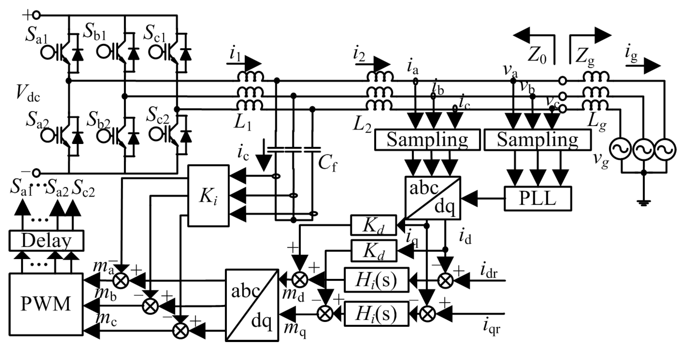
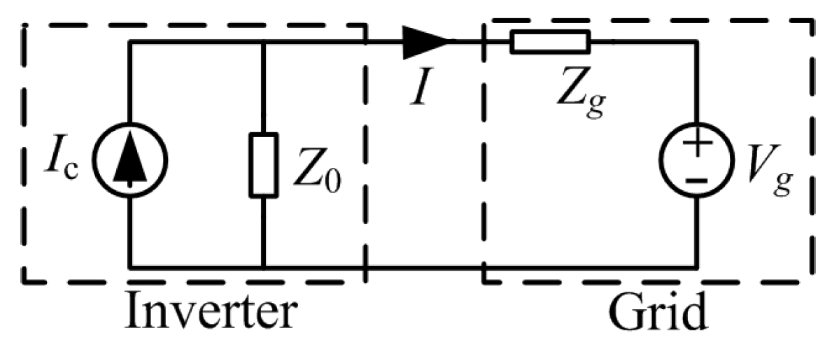
The grid-connected VSI with LCL-filter is depicted in
Figure 1. Phase voltages are denoted as
va,
vb, vc, while phase currents are represented by
ia,
ib, ic.
L1 and
L2 are the inverter-side inductor and grid-side inductor, respectively.
Cf is the filter capacitor. The capacitor current feedback loop is chosen to eliminate the high-frequency resonance resulting from the LCL filter,
Ki is the feedback coefficient.
Z0 denotes the inverter impedance and
Zg denotes the grid impedance.
Lg denotes the inductive component of the grid.
Figure 1 shows the
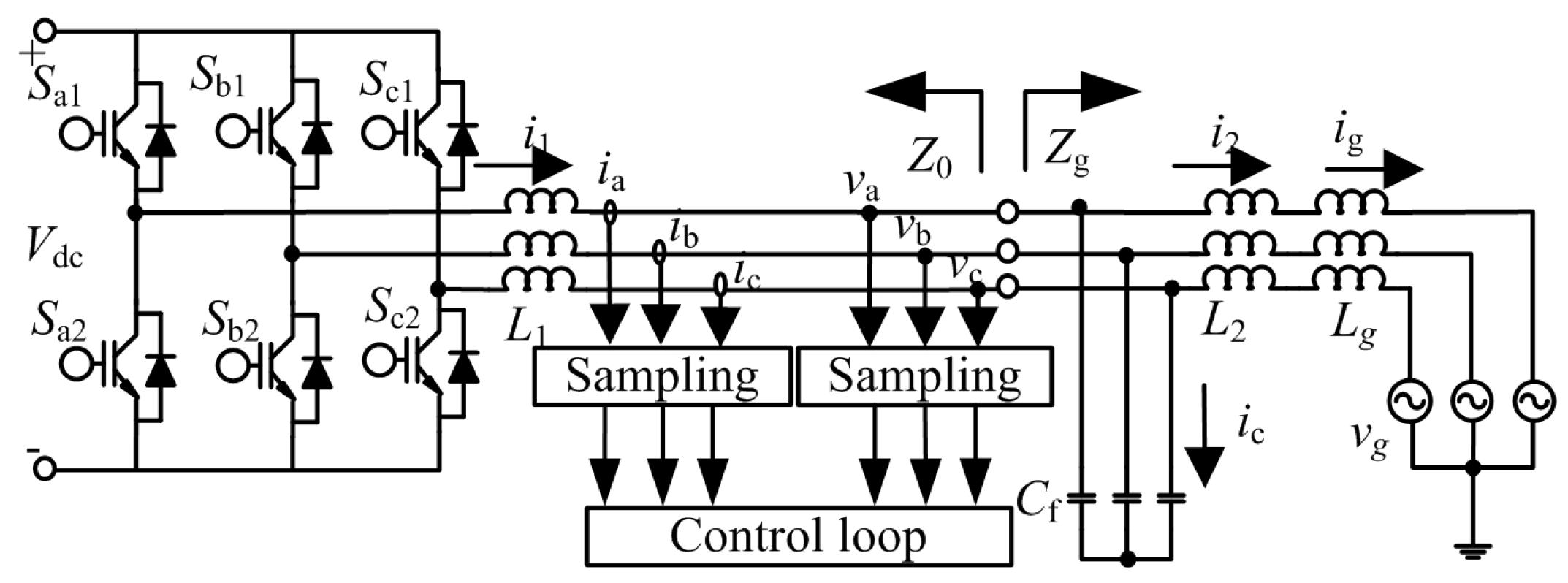
dq-domain GC feedback control. With regard to other control schemes,
Figure 2 depicts the IC feedback control, here
Cf and
L2 are considered as parts of the grid impedance expressed as
Zg.
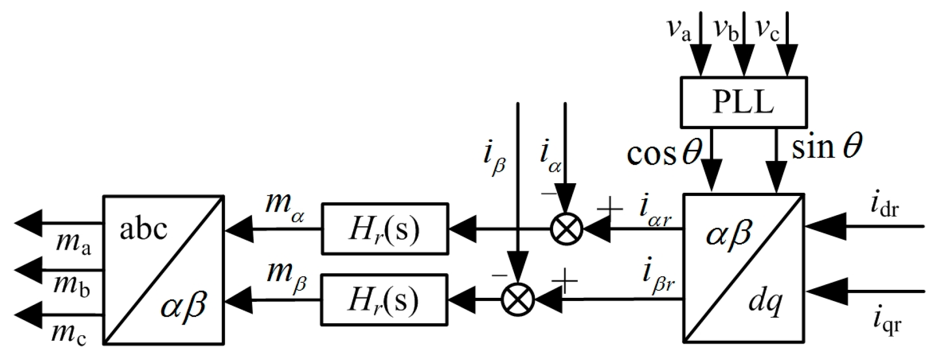
Figure 3 shows the αβ-domain current feedback control.
The harmonic linearization impedance modeling approach is based on the Fourier Transform. Specifically, apply a small positive- or negative-sequence voltage perturbation on the fundamental voltage at the point of common coupling (PCC) and find the corresponding response of the inverter currents at the same frequency of the superimposed perturbation. Then the impedance is defined as the ratio of the perturbed voltages to the corresponding currents [
10]. Here we take the modeling of positive-sequence impedance under
dq-domain GC feedback control as an example to introduce the modeling approach.
2.1. Impedance Modeling
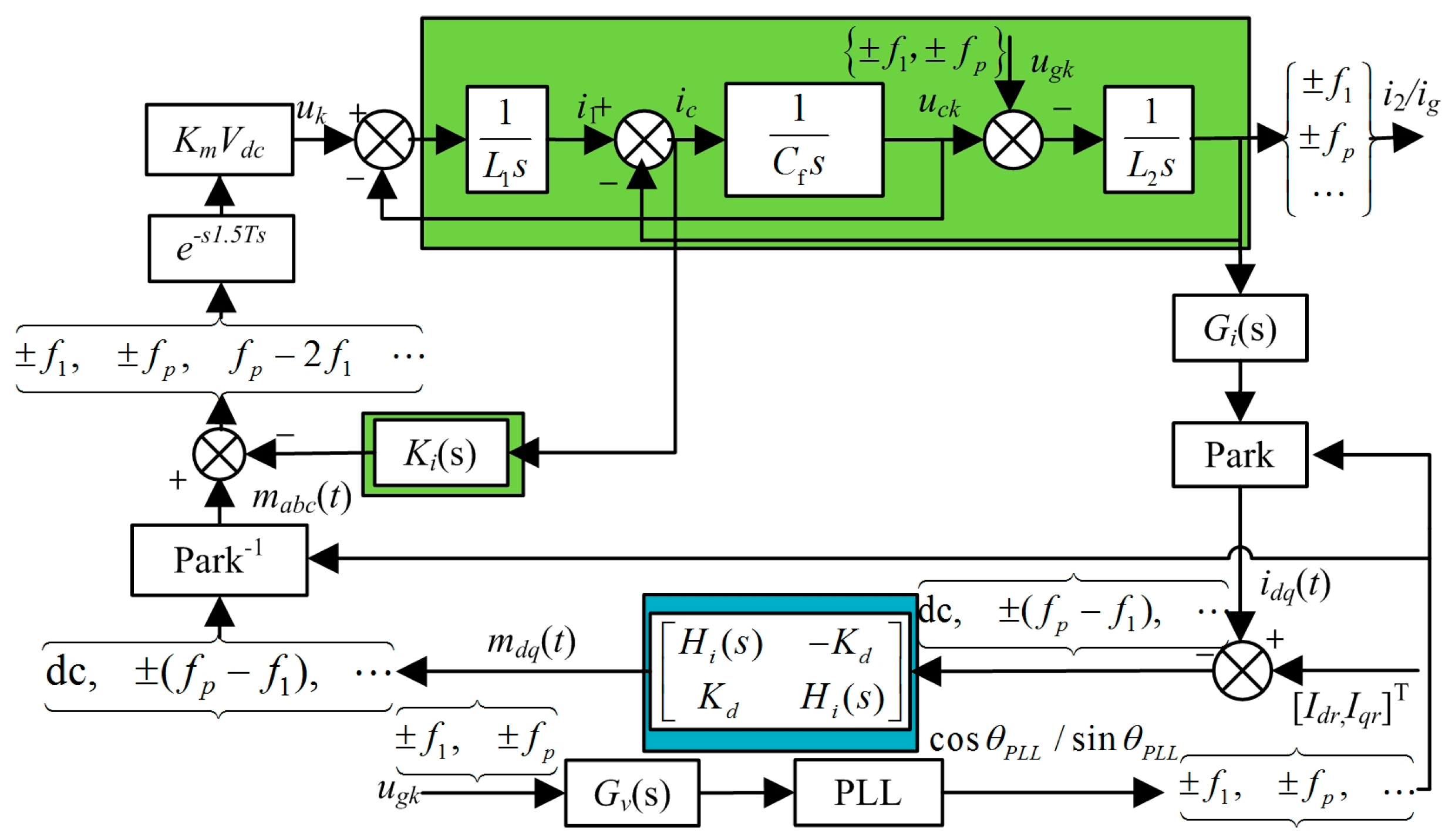
According to the harmonic linearization impedance modeling approach and the block diagram depicted in
Figure 1, when applying a small positive-sequence voltage perturbation on the fundamental voltage, we can get the positive-sequence signal flow diagram of inverter with
dq-domain GC feedback control shown in
Figure 4. In this figure
uk(s) is the output voltage at the inverter ac terminal,
uck(s) is the output voltage at the capacitor ac terminal,
ugk(s) is the output voltage at the grid ac terminal.
m is the modulating signals for PWM,
Km is the modulator gain.
Gv(s) and
Gi(s) model the voltage and current sampling delay.
Vdc is the dc bus voltage,
Idr and
Iqr are the reference currents. In modeling,
Vdc,
Idr,
Iqr is assumed constant.
f1 and
fp represent the frequencies of the signal and
fp is the frequency of positive-sequence perturbation.
In the time domain, the phase voltages with a small-signal positive perturbation can be written as:
where
V1 with
f1 is the amplitude and frequency of the fundamental voltage;
Vp,
fp and
is the amplitude, frequency and phase of the positive-sequence voltage perturbation. In the frequency domain, (1) can be written as:
where
Van[
f] is the Fourier transform of
va (t),
V1n[
f] and
Vpn[
f] are defined as:
Other phase voltages can be inferred from (2):
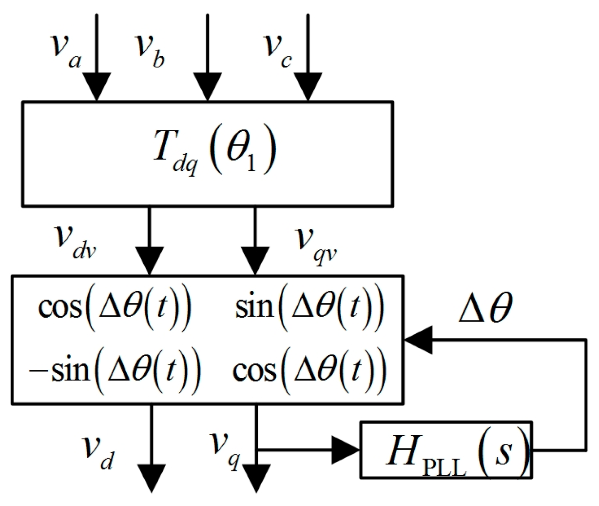
In order to find the current response under the positive-sequence voltage perturbation shown in (1), the first step is to derive the small-signal response of the phase-locked loop (PLL).
Figure 5 depicts the basic building block of a synchronous reference frame (SRF) PLL, where
is the phase of the grid voltage, and
HPLL(s) is the loop compensator. In order to solve the nonlinearity in Park’s transformation, we break
Figure 5 into two parts as depicted in
Figure 6, where
.
Introduce the frequency-domain Equations (2) and (4) into
Figure 6, the calculated lock signal in the frequency domain is written as follows:
Finally the following transfer function is found:
where
Tp(s) models the response of
to
Vp(s).
Similarly, for a negative-sequence perturbation, the transfer function is modeled as:
Introducing the small-signal response of PLL into
Figure 4, we can get the inverter output impedances under
dq-domain GC feedback control as in (9) and (10):
where:
and
is the complex conjugate of
,
is the complex conjugate of
I1.
I1 is the magnitude of fundamental current.
Under the
dq-domain IC feedback control, this is equivalent to the L-filter inverter shown in
Figure 2 [
10],
Cf and
L2 are considered as parts of the grid impedance, so the only difference in the signal flow diagram between GC and IC feedback is the green area illustrated in
Figure 4. Under the αβ-domain GC feedback control, the only difference of signal flow diagram between
dq- and αβ-domain control lies in the blue area depicted in
Figure 4. Similarly, their inverter output impedances are modeled as follows:
where:
and
is the complex conjugate of
.
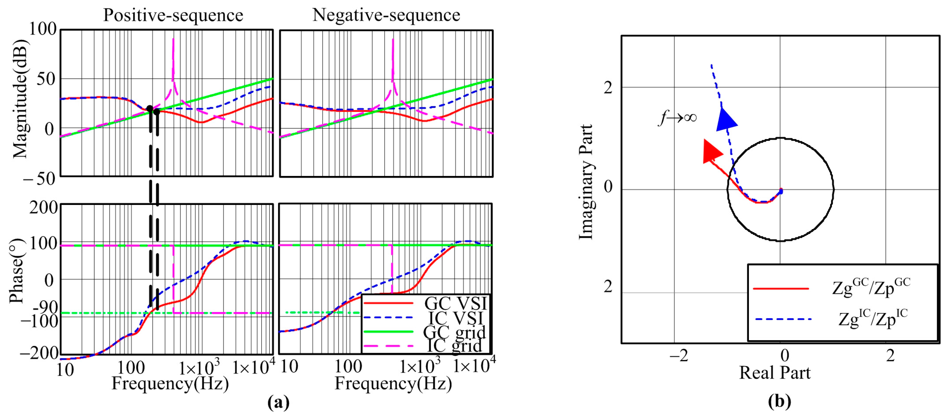
2.2. Impedance Models Verification
By means of Plecs, we apply a frequency sweep method to verify the modeled impedances. The parameters for the simulation are listed in
Table 1.
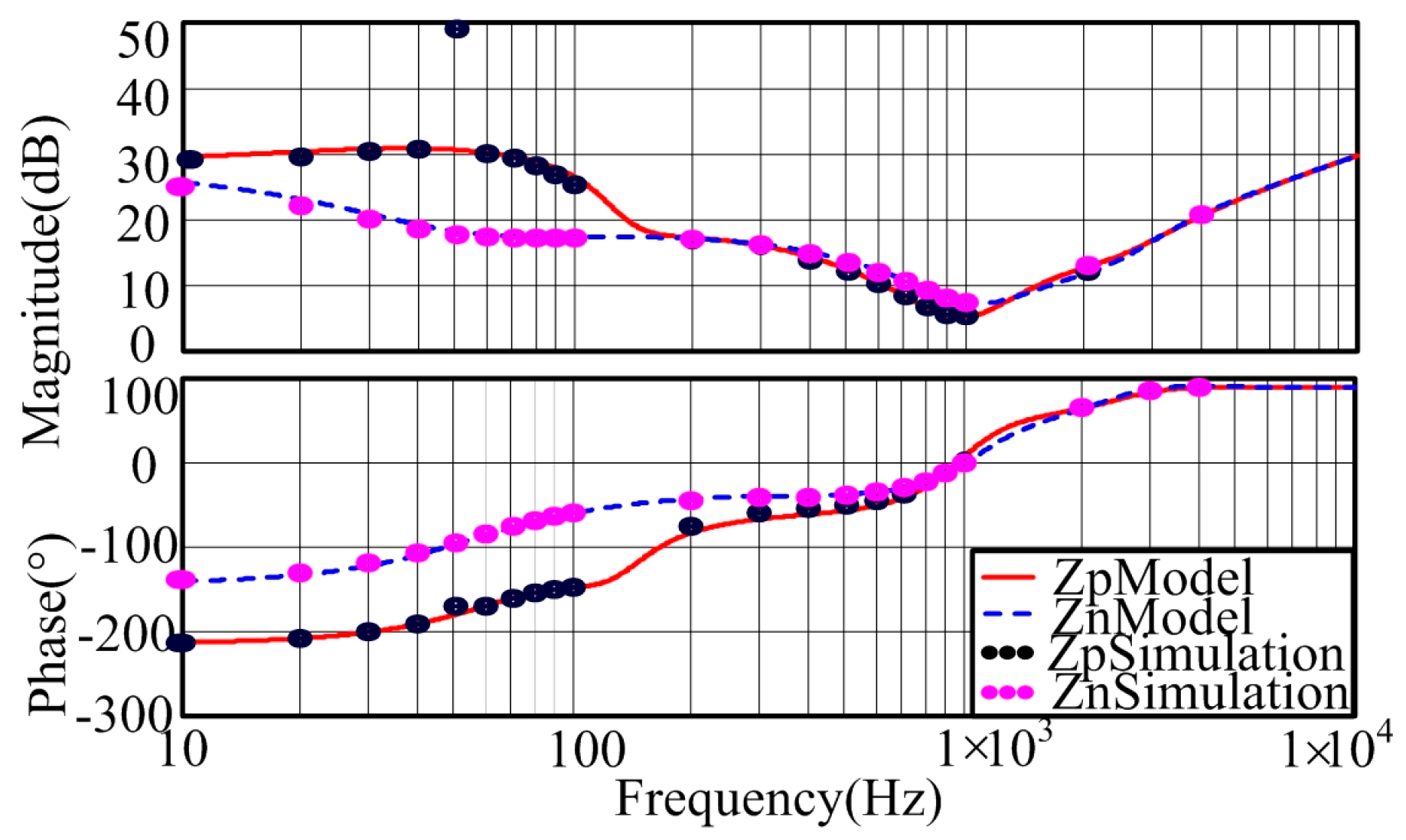
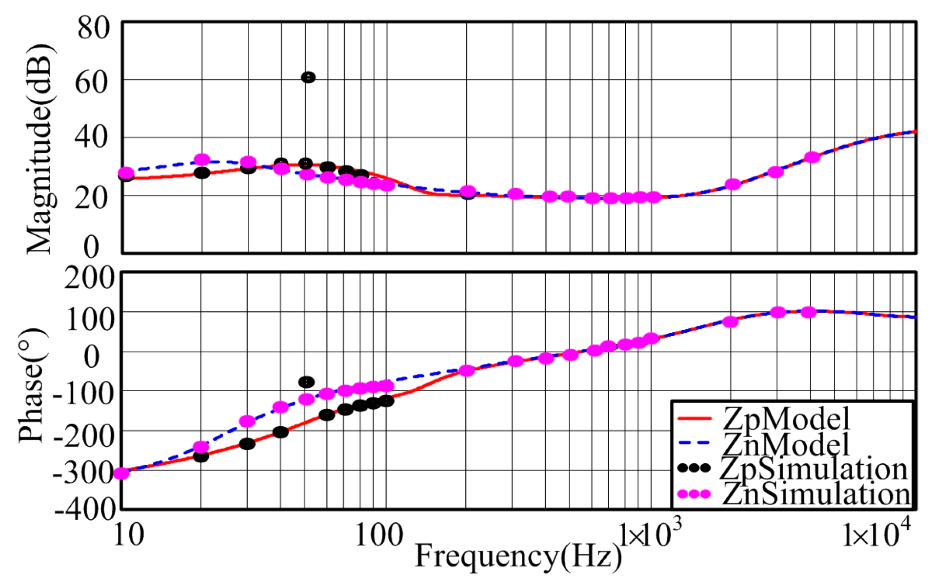
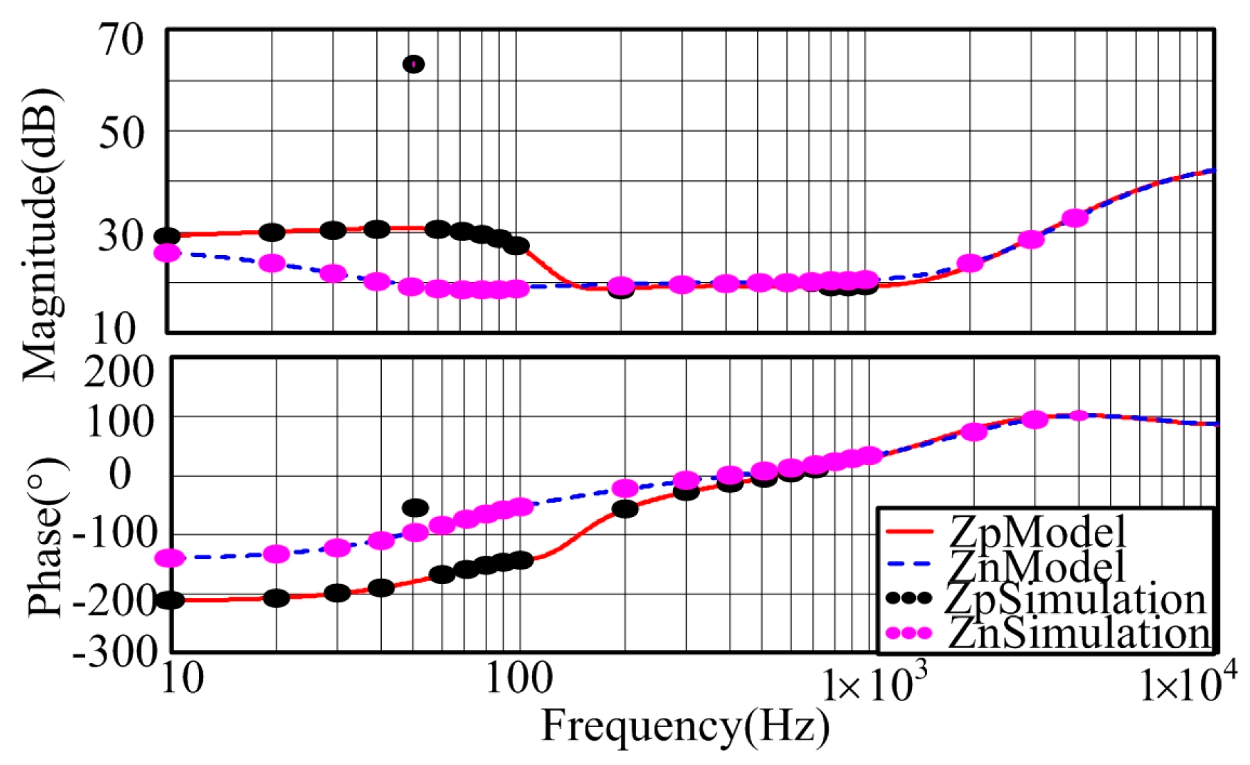
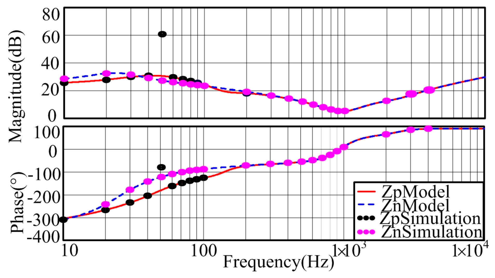
Figure 7,
Figure 8,
Figure 9 and
Figure 10 show the frequency response under different control schemes. The red solid line and the blue broken line represent the positive- and negative-sequence models, respectively; the black dashed line and the pink dashed line show the positive- and negative-sequence simulations, respectively. It can be concluded that the modeled impedances are verified well by the simulation, which validates the accurate modeling approach of the output impedances of the grid-connected inverters. It can be seen that differences between positive-sequence and negative-sequence impedance appear at lower frequencies; this is because of the shifting of effects of ±
jw1 that makes them different [
1]. Additionally, we can see that the main difference between GC and IC control lies at frequencies where
s >>
jw1 as seen comparing
Figure 7 with
Figure 8, or
Figure 9 with
Figure 10. The main difference between
dq- and αβ-domain control locates at lower frequencies, as seen by comparison of
Figure 7 with
Figure 9, or of
Figure 8 with
Figure 10.
2.3. Impedance Analysis
Different control schemes present some differences in their corresponding determined frequency ranges. In order to find out the reason why the output impedances show some differences, as depicted in
Figure 7,
Figure 8,
Figure 9 and
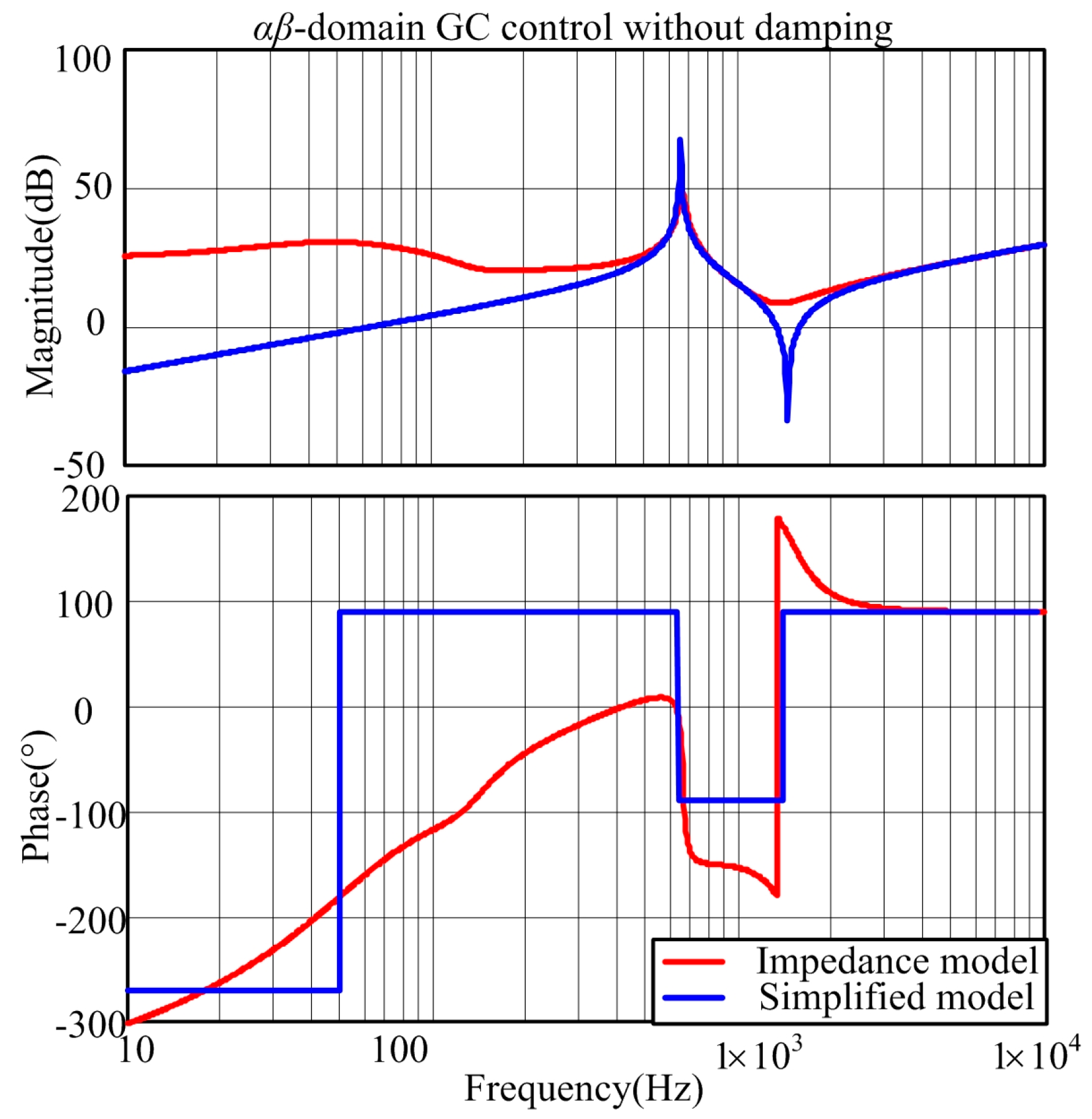
Figure 10, here we analyze the dominant factor(s) in different frequency ranges to recognize some existing resonance phenomena better and meanwhile demonstrate indirectly the main difference of different control schemes. Here we take the positive-sequence impedance under the αβ-domain GC feedback control as an example to characterize the impedance in the high, medium and low frequency ranges.
Referring to the high-frequency (>500 Hz) characteristics of the output impedance,
Figure 11 shows the comparison of the whole impedance model and the simplified model as in (22). The simplified model just considers the filter part. It can be concluded that the simplified model can describe the high-frequency impedance characteristics well, which indicates that high-frequency characteristics mainly lie in the filter.
As for the medium-frequency (200–500 Hz) characteristics of the output impedance,
Figure 12a shows the comparison of the whole impedance model as in (18) and the simplified model as in (23) derived from neglecting the PLL in (18).
Figure 12b depicts the impedance response with different current controller parameters. It can be seen that the simplified model can represent the medium-frequency impedance characteristic well, and the adjustment of current controller parameters has a great influence on the medium-frequency impedance characteristics [
1,
6], which illustrates that the medium-frequency characteristics are not related with PLL and they are determined mainly by the current controller parameters. Increasing the proportional and integral coefficients can improve the magnitude of the medium-frequency impedance greatly. However it deteriorates the phase in high-frequency range.
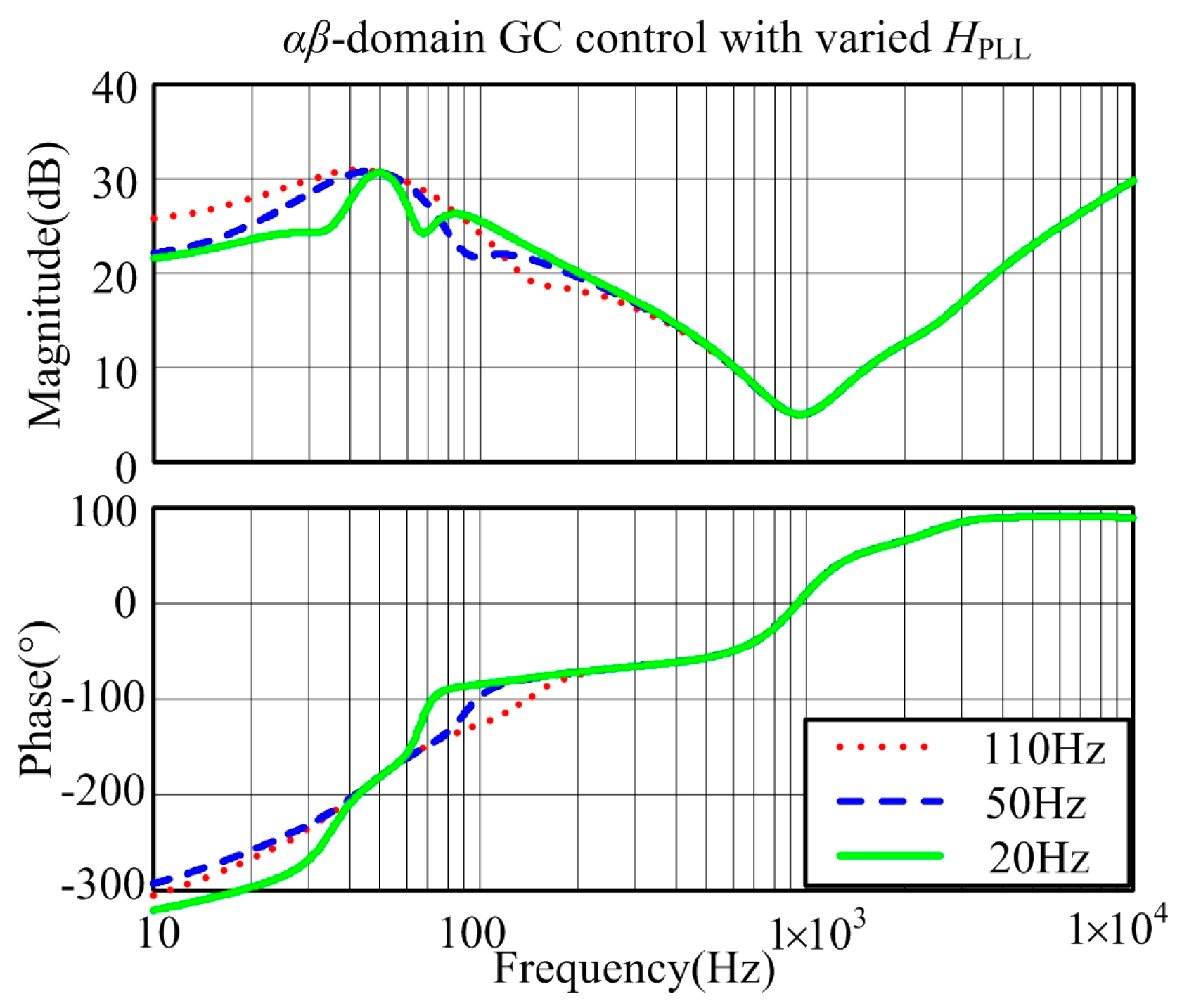
With regard to the low-frequency (30–200 Hz) characteristics of the output impedance,
Figure 13 depicts the impedance response with different PLL controller parameters. It can be seen that the adjustment of PLL controller parameters has a great influence on the low-frequency impedance characteristics [
1,
10]. Considering the results of
Figure 12b and
Figure 13, it reveals that PLL contributes a lot to the low-frequency characteristics. Decreasing the bandwidth of the PLL controller can improve the phase of the low-frequency impedance.
From the above analysis and considering the modeling process, since the difference between GC and IC feedback lies in the filter, it can be concluded that the essential difference under different current sampling schemes locates in the high-frequency range; as the main difference between αβ-domain control and
dq-domain control is the current control loop including the current controller and the PLL, the impedances under different reference frame present different characteristics both in medium- and low-frequency range. The theoretical results are consistent with the model comparison shown in
Figure 7,
Figure 8,
Figure 9 and
Figure 10.
4. Experimental Results
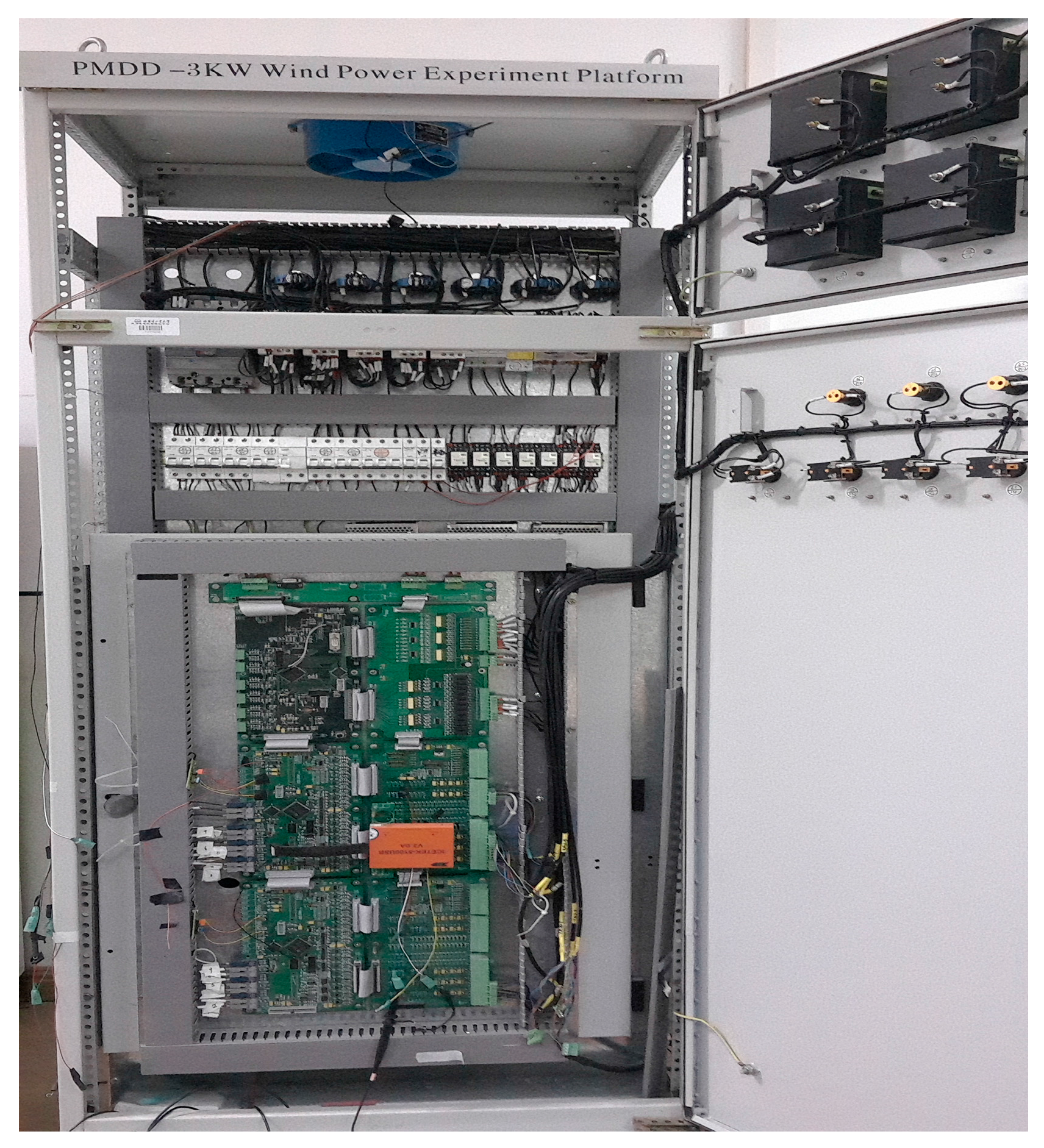
To confirm the theoretical analysis in
Section 3, a series of experiments were implemented on a 3 kW wind power experimental platform depicted in
Figure 17. On this platform, the grid inductor has values of 2, 4, 6, 8 and 10 mH. By choosing different values, we can simulate the variation of the grid impedance to compare the effects of different control schemes under weak grid conditions.
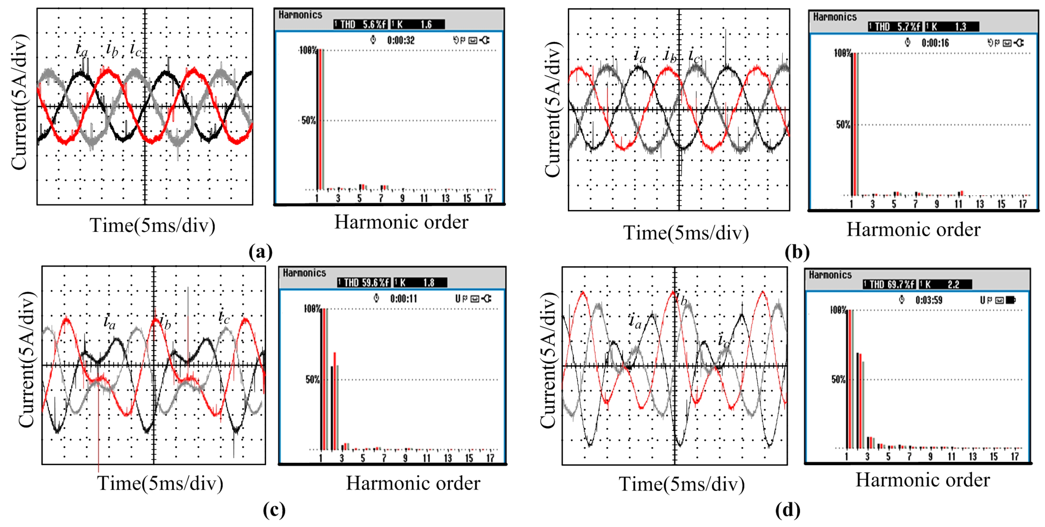
Figure 18 shows the stability comparison under different current sampling schemes, where it can be seen that when
Lg = 4 mH, the current waveform is sinusoidal under both the IC and GC sampling schemes, and when the grid inductor increases to 6 mH, the currents are resonant together, which indicates that different sampling schemes contribute little to the resonance resulting from varied grid impedance. Although the THD under IC sampling is smaller than in the GC sampling scheme, the difference is so small that it can be neglected.
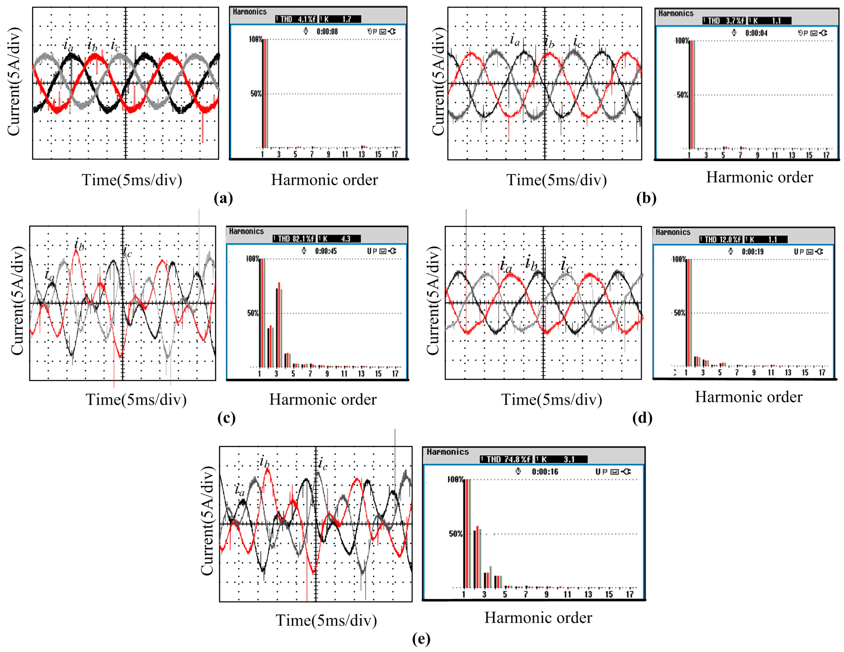
Figure 19 depicts the stability comparison with GC sampling under different current reference frames, where we can draw the conclusions that when
Lg = 2 mH, the current waveform is stable both under the
dq-domain and αβ-domain control schemes, that when the grid inductor increases to 4 mH, the currents display apparent resonance under
dq-domain control, and the currents under αβ-domain control become unstable when
Lg = 6 mH, which indicates that the αβ-domain control is more adaptable to the weak grid than
dq-domain control.
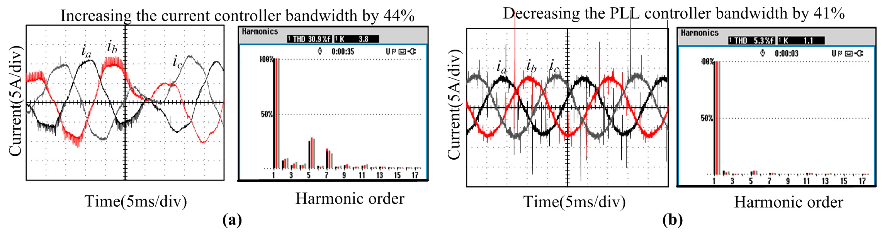
Aiming at eliminating the resonance seen in
Figure 19e,
Figure 20 compares the effects of regulating the current controller and PLL controller. It can be concluded that decreasing the PLL controller bandwidth by 41% can eliminate the resonance absolutely and increasing the current controller bandwidth by 44% can only improve the resonance phenomena, so decreasing the PLL controller bandwidth is more effective to improve the stability in inverter-grid systems.


