Revisiting Structural Modeling of Credit Risk—Evidence from the Credit Default Swap (CDS) Market

Abstract

The ground-breaking Black-Scholes-Merton model has brought about a generation of derivative pricing models that have been successfully applied in the financial industry. It has been a long standing puzzle that the structural models of credit risk, as an application of the same modeling paradigm, do not perform well empirically. We argue that the ability to accurately compute and dynamically update hedge ratios to facilitate a capital structure arbitrage is a distinctive strength of the Black-Scholes-Merton’s modeling paradigm which could be utilized in credit risk models as well. Our evidence is economically significant: We improve the implementation of a simple structural model so that it is more suitable for our application and then devise a simple capital structure arbitrage strategy based on the model. We show that the trading strategy persistently produced substantial risk-adjusted profit.

1. Introduction

“Seldom has the marriage of theory and practice been so productive.”

—by Peter Bernstein, financial historian, in Capital Ideas: The Improbable Origins of Modern Wall Street [1]

The quote above is a compliment to the ground-breaking Black-Scholes-Merton Model ([2,3]) and the rapidly developing generation of derivative pricing models. These models, with starry empirical performance that facilitated the mushrooming of the financial derivative markets, have brought the lending capacity of the financial industry to a new height.

However, this modeling paradigm faced major difficulties when it was applied to one of the oldest financial instruments—bonds. Merton [4] started this endeavor by pointing out that the value of a bond is the difference between the value of the underlying asset (value of the business) and a call option of the underlying asset, or equivalently, the difference between a riskless bond and a put option of the underlying asset. This key insight made the application of the Black-Scholes-Merton modeling paradigm to credit risk straightforward. The type of credit risk models that follow the Black-Scholes-Merton modeling paradigm are referred to “structural models of credit risk”.

A notable difficulty in empirical performance of the structural models is the so-called “credit spread puzzle”. The puzzle was first brought to light by Huang and Huang [5]. They concluded that credit risk accounts for only a small fraction of the observed level of yield spreads. Collin-Dufresne, Goldstein and Martin [6] examined the variables present in structural models and found that they only explained a small fraction of the variability in spreads. The puzzle has been intensely discussed; see for example [7,8,9,10,11].

There are at least two possible explanations for this puzzle. First, important aspect(s) in the default mechanism are missing from the model. Namely, Merton [4] told a straightforward economic story—a firm would default whenever its assets value fell below the debt level at maturity. Important details in that story might have been left out. More aspects of the credit default have been added to the story ever since. Black and Cox [12] allowed default to happen at any time before or at maturity. Longstaff and Schwartz [13] introduced the stochastic interest rate. Leland [14] introduced endogenous default, allowing default to be a strategic decision by the management. Leland and Toft [15] considered a firm trying to keep an optimal capital structure by choosing the amount and maturity of its debt. Dufresne and Goldstein [16] introduced the stationary leverage ratio.

However, these extensions, despite the valid and interesting perspectives they brought about, did not lead to material improvements in empirical performance, lending the first possible explanation limited support. Huang and Zhou [17] conducted a consistent specification analysis of structural credit risk models. Their empirical tests strongly rejected the Merton [4], Black and Cox [12], and Longstaff and Schwartz [13] models. Again in their test, Huang and Huang [5] outperformed the three but still was rejected for more than half of the sample. The best model considered in Huang and Zhou [17] was the stationary leverage model of Collin-Dufresne and Goldstein [16], which was not rejected in more than half of the sample. Huang and Zhou [17] further documented that none of the five structural models can capture the time-series behavior of both CDS spreads and equity volatility. Given that equity volatility in structural models is time-varying, they suggested that this finding provided direct evidence that a structural model with stochastic asset volatility may significantly improve model performance.

A second possible explanation is that factors unrelated to credit risk play a substantial role in the bond price; however, since they are non-credit related, they are excluded from the structural model. Huang and Huang [5] first suggested this potential explanation. Elton, Gruber, Agrawal, and Mann [18] provided empirical evidence that state tax explains a substantial proportion of the corporate bond spread. Chen, Lesmond, and Wei [19] provided empirical evidence that liquidity is indeed priced in both levels and changes of the yield spread.

Bao and Pan [20] compared the two explanations directly and provided strong evidence in favor of the latter. They documented that empirical volatilities of corporate bond and CDS returns are higher than is implied by equity return volatilities and the Merton model. They further documented some relation with variables proxying for time-varying illiquidity but little relation between excess volatility and measures of firm fundamentals and the volatility of firm fundamentals.

It is worth noting from this literature that such non-credit risk related factors can even influence credit derivatives like credit default swaps, which are supposedly “purer” instruments for credit risk. (See, for example, [20,21]).

The relevant question is, with the non-credit risk related factors influencing both the bond and the credit default swap, can structural models of credit risk still be put to good use?

Schaefer and Strebulaev [22] were among the first to say yes. Schaefer and Strebulaev [22] found that structural models of credit risk produce accurate hedge ratios. Specifically, a majority of the hedge ratios produced by a structural model are in line with the hedge ratios produced by time series regression.

Subsequently, the hedge ratio has been discussed by later study as a key to understand the weakness of structural models of credit risk. For example, Bao and Hou [23] use the hedge ratio to look into the heterogeneity in the co-movement of corporate bonds and equities. They found that bonds that are later in their firms’ maturity structure have higher hedge ratios, hedge ratios are larger for firms with greater credit risk within ratings. Their findings are consistent with the prediction of the extended Merton model. Huang and Shi [24] reconciled the “equity-credit market integration anomaly” from the perspective of the hedge ratio.

We argued that accurate computation of hedge ratio is only part of a bigger picture. A distinctive feature of the Black-Scholes-Merton modeling paradigm is the construction of a dynamic trading strategy aimed at exploiting pricing discrepancies among different securities of the same underlying asset. Such a trading strategy is called a capital structure arbitrage. The success of a capital structure arbitrage relies critically on the dynamic rebalancing of the portfolio which relies on the accurate computation and dynamic updating of the constantly changing hedge ratio. Namely, the accuracy and dynamic updating of hedge ratio is the key to a capital structure arbitrage.

We argue that the ability to accurately compute and dynamically update hedge ratios to facilitate a successful capital structure arbitrage is a distinctive strength of the Black-Scholes-Merton’s modeling paradigm which could be utilized in credit risk models as well. Consequently, a place where the structural model of credit risk performs well is the application related to capital structure arbitrage.

Empirically, we implemented a simple structural model of credit risk, which facilitated a capital structure arbitrage that persistently produced substantial risk adjusted profit.

Our empirical result is an improvement upon those of Schaefer and Strebulaev [22]. First, in Schaefer and Strebulaev [22], linear time series regression was used as the benchmark to “test” whether or not the hedge ratio produced by the structural model was accurate. The empirical result of their study was that the hedge ratios produced by the structural model and the linear time series regression models were not far apart (except for the AAA bonds). An immediate question is, since a linear regression model is much easier to implement than a structural model, and it is accurate enough to serve as the benchmark of hedge ratio calculation, what is the point of using a structural model at all? Second, the way the structural model was implemented in Schaefer and Strebulaev [22] actually largely eliminated the advantage of a structural model over a linear regression type of model. Specifically, every grade of bonds has only one hedge ratio, as an average of the hedge ratio of all the bonds of the same grade and cross time. However, one distinctive advantage of structural models is the capacity to dynamically recalculate the constantly changing hedge ratio of an individual firm, and such hedge ratios surely vary cross-sectionally, which is beyond the reach of linear regression types of models. Moreover, the problem may also go deeper than that: Although intuitively such “average” hedge ratios converge to certain “expected hedge ratio”, the way the model is implemented may fail. Namely, every time series has only one volatility estimate, which is an average volatility over time. One hedge ratio is calculated according to this average, and the hedge ratio is considered an average hedge ratio. However, the hedge ratio is a nonlinear function of volatility. The following equation was an implicitly assumption for the algorithm in Schaefer and Strebulaev [22]:

$$E(h((\mathsf{\sigma })))=h(E(\mathsf{\sigma }))$$

(1)

Equation (1) is true if h is a linear function of $\mathsf{\sigma }$ or $\mathsf{\sigma }$ is constant over time. In the case of a structural model, h is not linear, and apparently $\mathsf{\sigma }$ changes over time, therefore, Equation (1) is not true in general.

Our study overcomes all the limitations aforementioned in Schaefer and Strebulaev [22]. Instead of using a linear regression as a benchmark, we used the market as the benchmark—we utilized a structural model in a capital structure arbitrage trading, demonstrating substantial persistent risk adjusted profit. It is worth mentioning that our evidence is therefore economically significant, not just statistically significant. The hedge ratio is recalculated at every point in time for every firm, demonstrating the unique strength of the structural model, which would be difficult for a linear regression type of model to accomplish.

Our results do not suggest that all the shortcomings of structural models of credit risk are due to the non-credit risk related factors. Bao [25] found that the part of the cross-sectional variation unexplained by the Black-Cox model is related to credit risk proxies such as recent equity volatility, ratings, and option expensiveness. Further, Bao [25] found that unexplained yield spreads are related to unexplained CDS spreads.

We utilized option implied volatility as opposed to historical volatility to be one of the key inputs of the structural model. We do so because option implied volatility is capable of expressing new information incorporated in the options market, while historical volatility moves slowly. The advantage of option implied volatility has been discussed previously. For example, the information content of option implied volatility has been discussed in [26]. They used a linear regression approach to demonstrate that option volatility dominate historical volatility in explaining time series CDS spread. Cao, Yu and Zhong [26] did not use option implied volatility directly as an input to the structural model. Cao, Yu and Zhong [26] went one step further by using implied volatility as an input to the structural model. They demonstrated that the CDS spread provided by such an implementation matched the observed CDS spread better than using historical volatility as the input. Empirically, our study went yet one step further by providing economically significant evidence that a structural model with option implied volatility as an input can facilitate successful capital structure arbitrage.

In comparison with this literature, our data set is relatively old. However, the focus of our study is neither the information content of certain asset (options), nor the advantage of using one parameter over another. The focus of this study is to show whether or not structural model of credit risk can be put to good use despite all of the difficulties in credit risk modeling. Its working in one period in a certain way is good enough to make the point. A trading strategy should not be expected to work the same way all the time—it surely has to be modified according to changing regulatory environments, etc. The regulation around CDS trading has been through substantial changes and we surely would not expect the same trading strategy to work the same way all of the time.

The profitability of capital structure arbitrage has been discussed in previous studies; see, for example, [27,28,29]. Profit of their trading strategy was very modest, far less pronounced than that in our study.

This paper is organized as follows: Section 2 introduces the model used; Section 3 presents our improved implementation of the model; Section 4 describes the capital structure arbitrage based on the prediction produced by the model; Section 5 reports empirical test results; and Section 6 concludes.

2. The CreditGrades™ Model

The structural model we used in this study is the CreditGrades™ model [30]. It was developed jointly by the RiskMetrics Group, J.P. Morgan, Goldman Sachs, and Deutsche Bank. The CreditGrades™ model is a descendent of Black and Scholes [2] and Merton [4], wherein the equity is modeled as a call option on a firm’s assets, and the value of a firm’s debt is therefore the value of its assets in excess of the equity. One problem structural models encounter in pricing corporate bonds is that the predicted short-term credit spread is too low compared to market data. CreditGrades™ addresses this problem by introducing uncertainty in the default barrier, motivated by the fact that the market does not know the exact level of leverage of a firm except at the time when the firm actually defaults. This approach produces higher short-term spreads than those found in a typical structural credit risk model.

We choose the CreditGrades™ model here because it is simple in comparison with to the technically more sophisticated structural models. Good performance of a simple structural model helps to demonstrate the strength of structural models in general.

For detailed information of the model, please refer to the original CreditGrades™ technical document.

3. Improved Implementation

This section describes what distinguishes our implementation from conventional implementation.

The CreditGrades™ model provides a function f of externally observed (calculated) factors Z_t and model parameters β, to predict CDS spread Y_t at time t. Namely, the model predicts that Y_t = f (Z_t, β). Z_t, the vector of externally observed (calculated) factors, includes variables like stock price, stock return volatility, interest rate, etc.; β, the vector of model parameters, includes three elements: $\overline{L}$, $\mathsf{\lambda }$, and R1. For a detailed interpretation of the parameters, please refer to the original CreditGrades™ technical document.

In the original CreditGrades™ model technical documentation, $\mathsf{\lambda }$ and $\overline{L}$ are estimated to be 0.3 and 0.5, respectively, across all firms and all time, based on a study of historical data; bond specific recovery rate R is taken from a proprietary database from J.P. Morgan. In short, among the three unobservable parameters, $\mathsf{\lambda }$ and $\overline{L}$ take fixed values across firms and time while R varies across firm but is constant over time. In Yu [27], $\mathsf{\lambda }$ and R are fixed across firms and across time, while $\overline{L}$ is allowed to vary across firms but is constant over time. More specifically, as in Yu [27], $\overline{L}$ is estimated as the solution of the following programming:

$$\underset{\overline{L}}{{\displaystyle \min }}[{\displaystyle \sum _{t=1}^{10}{(f(Z_t,\mathsf{\lambda }=0.3,R=0.5,\overline{L})-y_t)}^2}]$$

In our implementation, we free up all three parameters—they are allowed to vary across firms and over time. In fact, the estimation is performed at every point of time t, with the most current data from the same firm, instead of estimating once and using the estimates forever, or using cross sectional data to estimate. Specifically, all the three model parameters are estimated as the solution of the following programming:

$$\underset{\mathsf{\lambda },R,\overline{L}}{{\displaystyle \min }}[{\displaystyle \sum _{s=1}^{25}{(f(Z_{t-s},\mathsf{\lambda },R,\overline{L})-y_{t-s})}^2}]$$

Namely, we modified the original implementation in the following way:

• Distinction 1:
  We freed up more model parameters. Instead of taking fixed values across firm and time, we allowed them to take the values that would allow the best match between the model and the data. The advantage of doing so is to allow the model more flexibility in expressing the firm-specific information in the data.
• Distinction 2:
  We re-estimated the model parameters at every point of time with the most current data of the same firm. The advantage of doing so is to allow the most current update of information be expressed.
• Distinction 3:
  In addition, one of the observable variables in Z_t is stock return volatility. Traditional implementation use historical volatility, for example, Yu [27]. We replaced historical volatility with option implied volatility. The advantage of using option-implied volatility is that option implied volatility reacts to new market information more promptly and in a more pronounced way, allowing the model to capture the newest information.

4. Capital Structure Arbitrage

This section provides a description of the capital structure arbitrage trading strategy.

4.1. Trading against the Market

The arbitrageur compares the real (market observed) CDS spread of an obligor and the theoretical CDS spread calculated based on the CreditGrades™ (CG) model and parameters obtained from the recent spread sheet, current stock price, current interest rate, maturity of the CDS spread, and, in some cases, the current price of the stock options of the obligator.

For a pre-specified threshold h, if the modeled spread c’ is higher than $(1+h)$ times of the realized spread c, namely,

$$c\prime >(1+h)\cdot c$$

(2)

the arbitrageur longs the CDS contract, which means she buys the insurance of the bonds and pays periodic premiums.

If the market spread c is higher than $(1+h)$ times of the model spread c’, namely,

$$c>(1+h)\cdot c\prime$$

(3)

the arbitrageur shorts the CDS contract, which means she sells the insurance of the bond and receives periodic premiums.

Why would this work? Suppose Equation (2) is true. That would be a signal that the market spread could be lower than its “fair” value, and it would tend to go up. Entering the long position of the CDS today means paying a lower than “fair” spread periodically for the insurance of the bond. Notice that the long position of the CDS contract is worth zero, just as is the short position of the same CDS contract at the time the CDS contract initiates. Sometime later, the market CDS spread might increase to its “fair” value. When this occurs, the market demands a higher periodic premium for the purchase of the same insurance. Now someone who needs to protect his/her bond value by entering the long position of a CDS spread will have to pay a higher periodic premium. She is willing to pay the arbitrageur a premium in exchange for the long position of the CDS contract, so that she can pay a lower periodic premium for the same protection. The situation when Equation (3) comes true is similar and will not be detailed here.

The “fair” value today may no longer be “fair” tomorrow simply because the underlying economic elements, such as stock price and volatility of stock return, etc., change. Therefore, profit is not guaranteed whenever the theoretical value and the real value converge. The theoretical value and the market value can fluctuate up and down together simply due to the change of underlying economic elements and converge at a value that makes the arbitrageur lose money.

Formally, suppose the theoretical CDS spread is given by $c_t\prime =f(S_t,{\mathsf{\sigma }}_t;{\mathsf{\vartheta }}_t)$, a function of the stock price $S_t$, asset volatility ${\mathsf{\sigma }}_t$ and a vector of other parameters ${\mathsf{\vartheta }}_t$. The real CDS spread is given by $c_t=c_t\prime -m_t$, where $m_t$ measures miss-price.

The arbitrageur assumes that $m_t$ cannot stay positive (negative) forever. Formally,

$$\underset{L\to \infty }{\lim }P(m_{t+L}\ge 0|m_t<0,m_{t+1}<0,\mathrm{...}{m}_{t+L-1}<0)=1$$

$$\underset{L\to \infty }{\lim }P(m_{t+L}\le 0|m_t>0,m_{t+1}>0,\mathrm{...}{m}_{t+L-1}>0)=1$$

With the above assumption assuring the convergence, the arbitrageur still cannot expect $c_t\prime =f(S_t,{\mathsf{\sigma }}_t;{\mathsf{\vartheta }}_t)$ or $c_t=c_t\prime -m_t$ to stay still while the underlying economic elements $(S_t,{\mathsf{\sigma }}_t;{\mathsf{\vartheta }}_t)$ are constantly changing. In the previous example, the arbitrageur enters a long position of CDS when ${c_t}^{\prime }>(1+h)\cdot c_t$. The arbitrageur can expect $m_t$ to come back down to zero, but when it does, both $c_t\prime =f(S_t,{\mathsf{\sigma }}_t;{\mathsf{\vartheta }}_t)$ and $c_t=c_t\prime -m_t$ may have gone up, which leaves the arbitrageur in a money-losing situation.

4.2. Delta Hedge

To hedge against the movement of CDS spread, stock is introduces into the portfolio. The hedge ratio here is the ratio between the change of the value of the CDS position and the change of the stock price, in a sufficiently short period of time. Intuitively, when the stock price increases (decreases), the CDS spread tends to decrease (increase), consequently, the value of a long CDS position will decrease (increase), therefore, it makes sense to have a number of short (long) position of the stock in the portfolio, to offset the impact from the stock price change to the value of the long CDS position.

Suppose that the long position of CDS maturing at time T is worth $\mathsf{\pi }(S_t,{\mathsf{\sigma }}_t;{\mathsf{\vartheta }}_t)$. The value change of the long position due to the change of stock price $S_t$, with the vector of other parameters ${\mathsf{\sigma }}_t$ and ${\mathsf{\vartheta }}_t$ holding constant is

$$\Delta \mathsf{\pi }(S_t,{\mathsf{\sigma }}_t;{\mathsf{\vartheta }}_t)=\frac{d\mathsf{\pi }(S_t,{\mathsf{\sigma }}_t;{\mathsf{\vartheta }}_t)}{d{S}_t}\Delta S_t+\mathsf{o}(\Delta S_t)$$

which implies $\Delta \mathsf{\pi }(S_t,{\mathsf{\sigma }}_t;{\mathsf{\vartheta }}_t)-\frac{d\mathsf{\pi }(S_t,{\mathsf{\sigma }}_t;{\mathsf{\vartheta }}_t)}{d{S}_t}\Delta S_t\approx 0$.

To hedge, the arbitrageur needs to purchase $-\frac{d\mathsf{\pi }(S_t,{\mathsf{\sigma }}_t;{\mathsf{\vartheta }}_t)}{d{S}_t}$ units of stocks to implement $-\frac{d\mathsf{\pi }(S_t,{\mathsf{\sigma }}_t;{\mathsf{\vartheta }}_t)}{d{S}_t}\Delta S_t$. (The arbitrageur needs to short sell $\frac{d\mathsf{\pi }(S_t,{\mathsf{\sigma }}_t;{\mathsf{\vartheta }}_t)}{d{S}_t}$ units of stock if $-\frac{d\mathsf{\pi }(S_t,{\mathsf{\sigma }}_t;{\mathsf{\vartheta }}_t)}{d{S}_t}$ is negative.)

The hedge does not provide complete protection of the portfolio because $S_t$ is not the only changing economic element that plays a role in the CDS spread. Other parameters that affect CDS spread can fluctuate over time and therefore bring changes to the value of the portfolio. Additionally, the speed at which $m_t$ converges to zero is important. If $m_t$ converges slowly, extended holding time comes with direct holding cost, and also more chances that the underlying value changes adversely. Additionally, when $m_t$ goes further from 0 to a large extent before converging, such a situation might force the arbitrageur to liquidate.

5. Empirical Tests

This section offers empirical tests of the performance of our improved implementation of the CreditGrades™ model. One distinctive feature of this study is that performance is measured by the profitability of the capital structure arbitrage (CSA) based on the implementation. Consequently, evidence produced would be economically significant. In what follows, Section 5.1 describes the data and explains how profitability is measured; Section 5.2 compares our improved implementation and conventional implementation; Section 5.3 assesses the profitability of CSA based on our improved implementation; and Section 5.4 assesses the persistence of the profitability of CSA based on our improved implementation.

5.1. Data and Computation of Profit

The CDS spread this study uses is the mid quote CDS spread of a five-year CDS contract on senior unsecured debt of North American Industrial Obligors from January 2001 to June 2004. The CDS data is merged with equity price and adjusted equity return data from CRSP and accounting information from Compustat quarterly data. Five-year U.S. treasury yields and three-month T-bill rates are from the Center for Research in Security Prices (CRSP). Option data come from OptionMetrics.

The above data merge and yield 178 investment grade firms and 35 speculative grade firms, with daily data in the period from January 2001 to June 2004. The total number of observations is 138,815. Basic statistics of the data are presented in

Table 1. Number of observations and market cap.

	Average	Median	Min	Max	Std	Total
Inv. Nob	641	648	377	867	136	114,073
Inv. Mkt cap	12.13B	9.21B	0.51B	301.72B	40.36B	4295.92B
Spec. Nob	707	739	468	873	119	24,742
Spec. Mkt cap	11.65B	4.62B	0.39B	75.56B	16.99B	407.81B

Note: Inv. Nob is the number of observation of investment grade firms. Inv. Mkt cap is the market cap of investment grade firms. Spec. Nob is the number of observations of speculative grade firms. Spec. Mkt cap is the market cap of speculative grade firms. Unit “B” represents one billion dollar.

and

Table 2. Industrial composition.

Sector	Count	Percentage
Communications and Technology	26	12.21
Consummer Cyclical	58	27.23
Consumer Stable	43	20.18
Energy	19	8.92
Industrial	44	20.66
Materials	23	10.8

Note: Table 2 presents the industrial composition of the obligors. Firms in the financial industry are excluded because their capital structure is hard to interpret.

.

The Fama-French Risk Factors and Momentum risk factors used in regressions are downloaded from Kenneth French’s data library online. For a detailed description, please refer to French’s online library [31].

The other four risk factors used in Yu [27] are from Datastream:

RSPIND	excess return on the S&P Industry Index, proxying for equity market risk
RINV	the excess return on the Lehman Brothers Baa intermediate index, proxying for investment grade bond market risk
RSPEC	Lehman Brothers Baa intermediate index, proxying for speculative grade bond market risk
RARB	excess return on the CSFB/Tremont Fixed Income Arbitrage Index proxying for the variations in the monthly excess returns not related to the market indices

Data of Option Implied Volatility: The structure of the option data is irregular: Some stocks have more related options than others. The largest number of options related to a stock in a single day is thirty-six. Additionally, the number of options related to a stock can be different from day to day. We calculate option-implied volatility by minimizing least square error. Namely, suppose at a certain date t, a stock (with stock price $s_t$) has $n$ related call options $(C_{1,t},C_{2,t},\mathrm{...}{C}_{n,t})$ with their strike price $(K_{1,t},K_{2,t},\mathrm{...}{K}_{n,t})$ and maturity $({\mathsf{\tau }}_{1,t},{\mathsf{\tau }}_{2,t},\mathrm{...}{\mathsf{\tau }}_{n,t})$. Suppose also that the risk-free interest rate is $r_t$. The Black-Scholes formula to calculate call option price $C$ from volatility $\mathsf{\sigma }$ is $C(\mathsf{\sigma },s,\mathsf{\tau },K,r)$. We implement the following optimization:

$$\underset{\mathsf{\sigma }}{{\displaystyle \min }}{\displaystyle \sum _{i=1}^n{(C_{i,t}-C(\mathsf{\sigma },s_t,{\mathsf{\tau }}_{i,t},K_{i,t},r_t))}^2}$$

The interest rate used above is the 3-month treasury rate. The solution of the above optimization ${\mathsf{\sigma }}_t$ is the implied option volatility needed to further calculate the asset volatility.2

Transaction Costs: A 5% bid-ask spread is assumed for the trading of CDS. For example, for a CDS spread quoted as 100 bps, the arbitrageur would have to pay 102.5 bps annually if she buys the contract; she receives annually only 97.5% bps if she sells the CDS contract. Stock trading is assumed to have no transaction cost.

Initial Capital: Every trade starts with an initial capital of $0.5 and a position in CDS with a $1.00 notional amount.

Index Return: We build our investment/speculative grade CSA index in the following way. We consider every trade to be carried out by a different hedge fund. The fund starts when the trade starts; it liquidates when the trade liquidates. We define investment/speculative grade CSA index as the equally weighted portfolio of all such hedge funds that hold investment/speculative grade CDS positions. The daily return of the index is then the average of the daily return of all hedge funds in the index. It is worth noting that the number of hedge funds in the index can change from time to time due to the creation of new hedge funds and the termination of old hedge funds. We then compound the daily return of the indexes into monthly return of the index.

Individual Trade Return: Suppose a trade starts at t and ends at T, with the values of portfolio being $V_t$ and $V_T$, respectively_. The excess return (ER) of the trade is then $\frac{V_T-V_t}{V_t}$ minus the return of the 3-month T-bill over period $(t,T)$.

The AER of an individual trade is the annualized excess return of the trade. Namely, $AER=\frac{ER}{(T-t)}\cdot 252$.3

Measures of Profitability: Various statistics are used to measure profitability, namely, Sharpe ratio, proportion of months of positive excess return, proportion of trades of positive excess return, proportion of trades with 20% drawdown, proportions of trades with modeled CDS spread and real CDS spread converged, and mean/skewness of the AER across trades.

5.2. Advantage of Our Improved Implementation over Conventional Implementation

In this section we makes two comparisons to show the incremental advantages of the distinctions of our improved implementation.

First, we define the capital structure arbitrage based on conventional implementation of CreditGrades™ model as TS04. Define the implementation with only Distinction 1 and Distinction 2 of our improved implementation as Implementation 1 and the CSA based on Implementation 1 as Trading Strategy 1 (TS1). We study the difference in profitability between TS1 and TS0.

Second, we define the CSA based on our improved implementation with all its three distinctions as Trading Strategy 2 (TS2) and study the difference in profitability between TS2 and TS1.

Third, we compare TS2 and TS0 directly.

5.2.1. TS1 vs. TS0

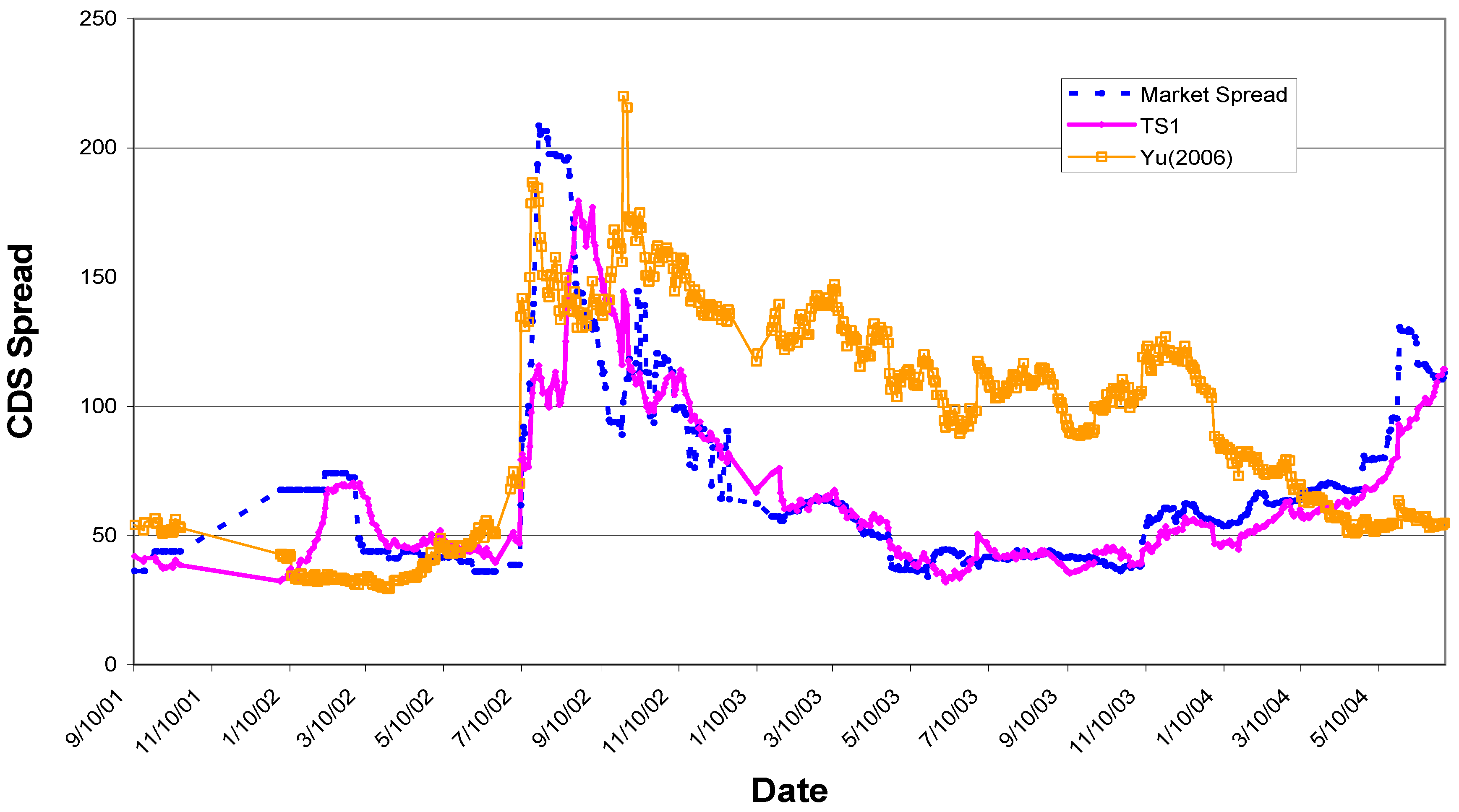
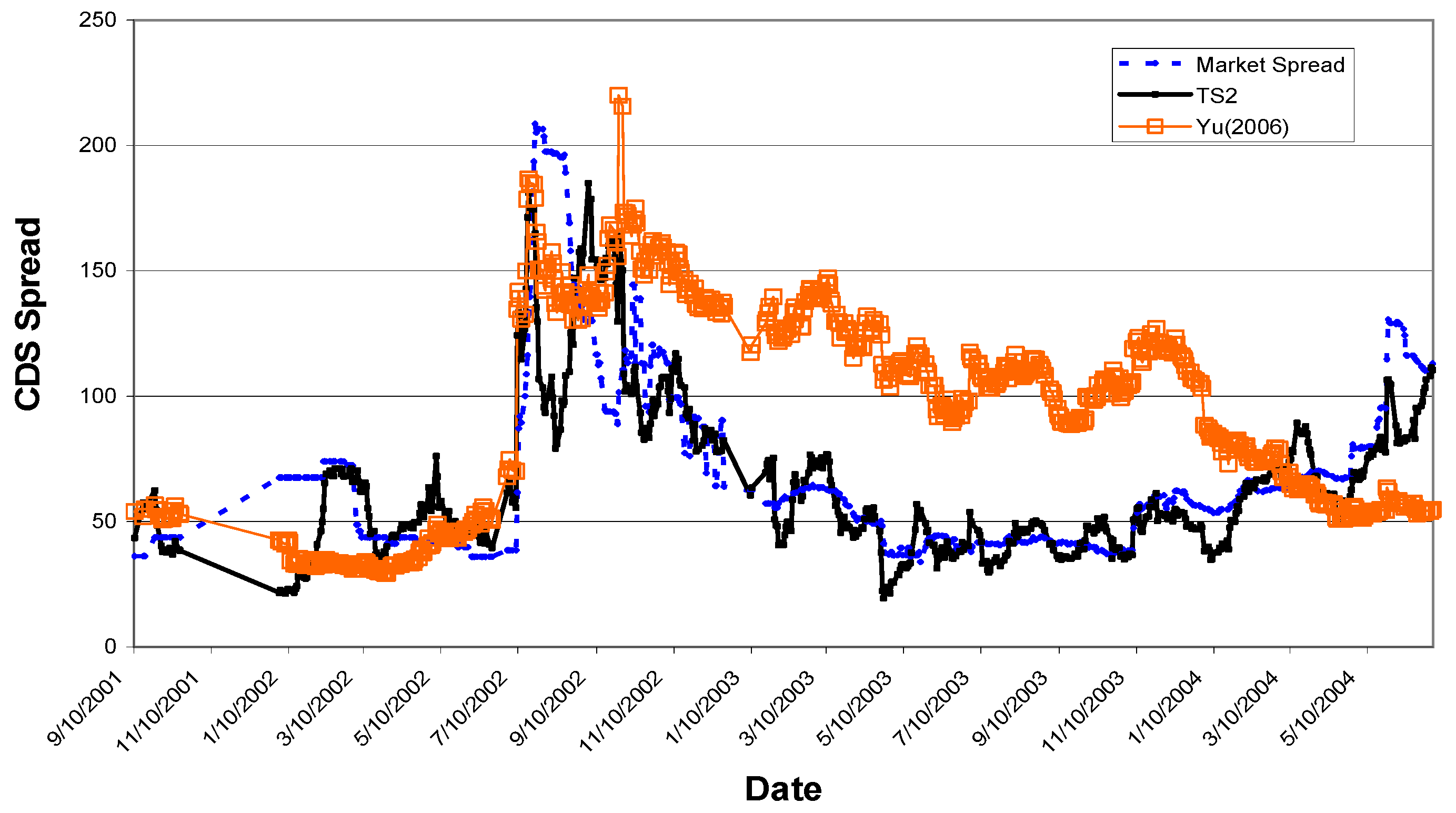
Before a systematic comparison, let us look into an individual firm to provide an intuitive perspective. The firm we will look at is Wyeth, a major drug manufacturer based in Madison, New Jersey. Wyeth engages in the discovery, development, manufacture, distribution, and sale of pharmaceuticals, consumer healthcare, and animal health products. It operates through three segments: Pharmaceuticals, Consumer Healthcare, and Animal Health. Famous products of Wyeth include Robitussin, Advil (ibuprofen), Premarin, and Effexor.

As Figure 1 demonstrates, TS1 has a much tighter fit than Yu [27]. Yu [27] persistently over-estimates market realized CDS spread for an extended period from 30 August 2002 to 3 March 2004. In the middle of the period, the fit is far off. At $threshold=0.5$, Yu [27] initiates 395 trades, with an average AER at 4.94%, while TS1 initiates only 34 trades, with an average AER at 20.28%, four times that of Yu [27]. All the trades TS1 initiates converge while only 38% of the trades Yu [27] initiates converge.

The statistical results of a systematic comparison between TS1 and Yu [27] are presented in

Table 3. TS1 vs. Yu [27].

Grade	Measure of Profitability	Estimate	StdErr	t-stat	p-Value
Investment	Sharpe Ratio **	1.19	0.17	7.13	<0.0001
	Positive Months **	0.17	0.02	8.22	<0.0001
	Positive Trades **	0.3	0.03	11.28	<0.0001
	Mean of AER **	0.32	0.032	10.37	<0.0001
	Skewness of AER **	−155.25	52.9	−2.94	0.0055
	Converged Trades **	0.91	0.02	50.5	<0.0001
	20% drawdown Trades	−0.000013	0.001	0.01	0.5
Spececulative	Sharpe Ratio **	0.94	0.29	3.3	0.001
	Positive Months *	0.07	0.05	1.58	0.0606
	Positive Trades **	0.3	0.07	4.5	<0.0001
	Mean of AER **	4.44	0.79	5.76	<0.0001
	Skewness of AER **	381	19.68	19.43	<0.0001
	Converged Trades **	0.91	0.01	67.49	<0.0001
	20% drawdown Trades	−0.00332	0.0124	−0.27	0.4

Step 1:

For every threshold h, simulate both TS1 and Yu [27] and compute the difference between their Sharpe ratios D_h.5 This step produces the series of D_h, with h ranging from 0.5 to 1.5.

Step 2:

Test hypothesis ${\mathrm{H}}_0:\mathrm{E}\left({\mathrm{D}}_h\right)=0 v.s.$${\mathrm{H}}_{\mathrm{a}}:\mathrm{E}\left({\mathrm{D}}_h\right)>0$.

In Step 2, we cannot use a straightforward T-test because the series D_h is auto correlated.6 Instead, we use an intercept-only regression and adjust for serial correlation in the error term with Newey-West adjustment:

$$\text{Regression}: {\mathrm{D}}_h=\mathsf{\alpha }+{\mathsf{\epsilon }}_h \text{with} E({\mathsf{\epsilon }}_h)=0 \text{for all} h$$

The hypothesis is now on the intercept $\mathsf{\alpha }$: ${\mathrm{H}}_0:\mathsf{\alpha }=0vs.$ ${\mathrm{H}}_{\mathrm{a}}:\mathsf{\alpha }>0$.

Step 3:

Repeat Step 1 and Step 2 but replace Sharp ratio with other measures of profitability, including the proportion of months with positive excess return, proportion of trades with positive excess, mean, and skewness of the AER across trades, proportion of trades that converges, and proportion of trades with a 20% drawdown7. For proportion of trades with a 20% drawdown, the alternative hypothesis needs to be changed to ${\mathrm{H}}_{\mathrm{a}}:\mathsf{\alpha }<0$.

Table 3 reports the estimate, standard deviation, t-statistics, and the p-value of the intercept in the regression.

For the skewness of the AER across trades in the investment grade CSA index, since the estimate is negative, the alternative hypothesis has to be changed to ${\mathrm{H}}_{\mathrm{a}}:\mathsf{\alpha }<0$. Rejection of the corresponding null hypothesis is interpreted as TS1 underperforms Yu [27] in the corresponding measure of profitability.

Items with ** have a confidence level of more than 99%. Items with a single * have a confidence level of more than 90%. TS1 outperforms Yu [27] in 11 measures and underperforms it in one measure at confidence of at least 90%. In general, TS1 outperforms Yu [27].

, and the statistical procedure is described in the caption of the table.

The conclusion we draw in this section is, for investment grade firms, in comparison with Yu [27], TS1 has a statistically significantly higher Sharpe ratio, higher proportion of trades and months with positive excess, higher mean average AER across trades, and higher proportion of trades that converge. For speculative grade firms, in comparison with Yu [27], TS1 has statistically significantly higher Sharpe ratio, higher proportion of trades with positive excess, higher mean and skewness of AER across trades, and higher proportion of trades that converge.

It is worth noting that for investment grade index, the skewness of the AER across trades of TS1 is actually statistically less than that of Yu [27]. The proportion of months with positive excess return in TS1 is statistically significantly larger than that in Yu [27] but only at a significant level of 94%. For both investment grade and speculative grade indexes, the proportion of trades with 20% drawdown in TS1 is not statistically different from that in Yu [27].

5.2.2. TS2 vs. TS1

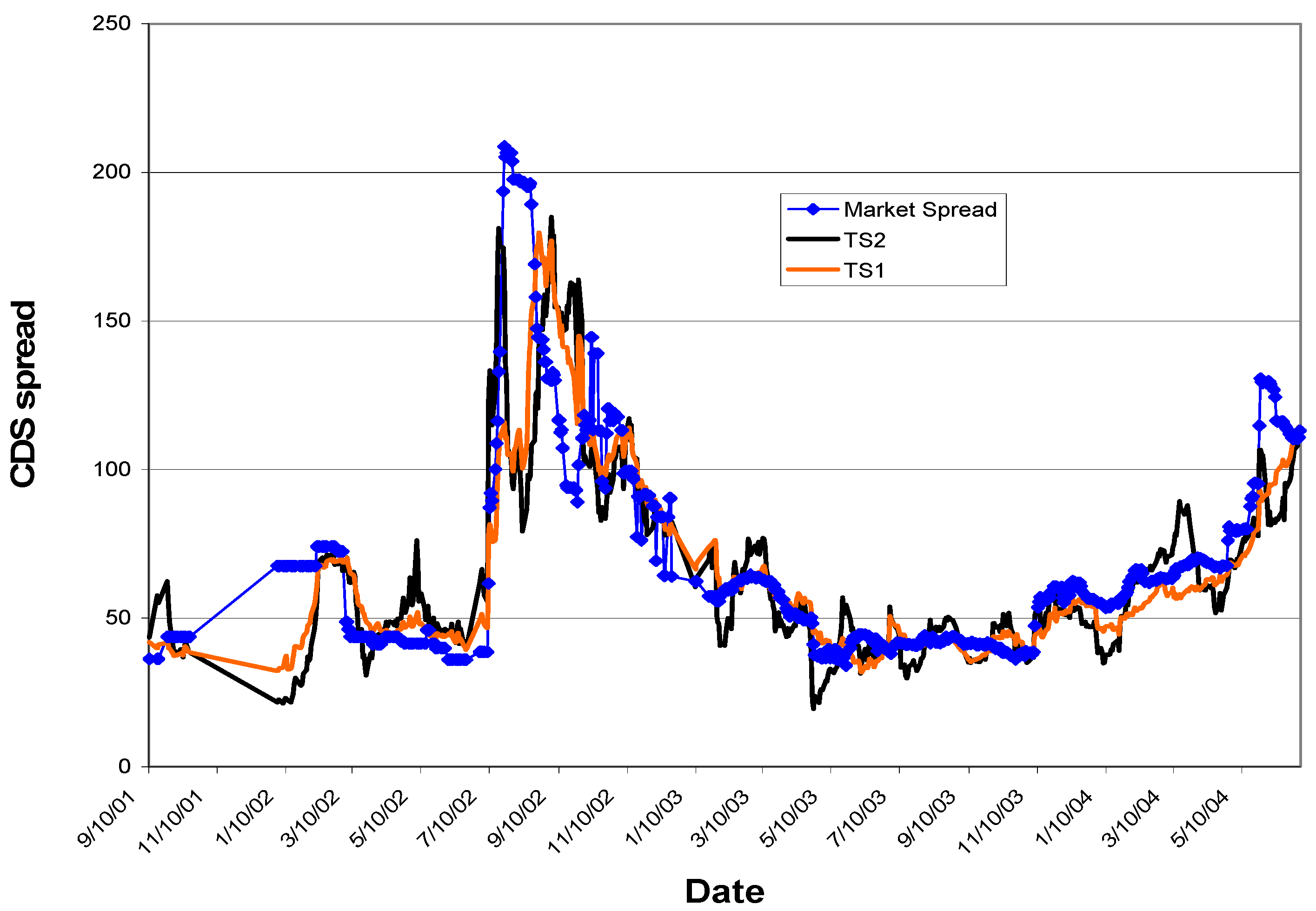
This section compares the profitability of TS2 and TS1. Before a systematic comparison, we again use Wyeth to provide an intuitive perspective. Figure 2 demonstrates the fit of both TS1 modeled spread and TS2 modeled spread. The TS1 model spread smoothly follows the market realized spread while TS2 model spread has more sudden large moves. TS2 gives more trading signals than TS1. At $threshold=0.95$, TS2 gives 34 trading signals while TS1 gives only 13. Among the 13 trading signals given by TS1, 11 are also given by TS2. (All the trading signals of both trading strategies are profitable.) The AHPERR is 1.9% for TS2 and 1.2% for TS1.

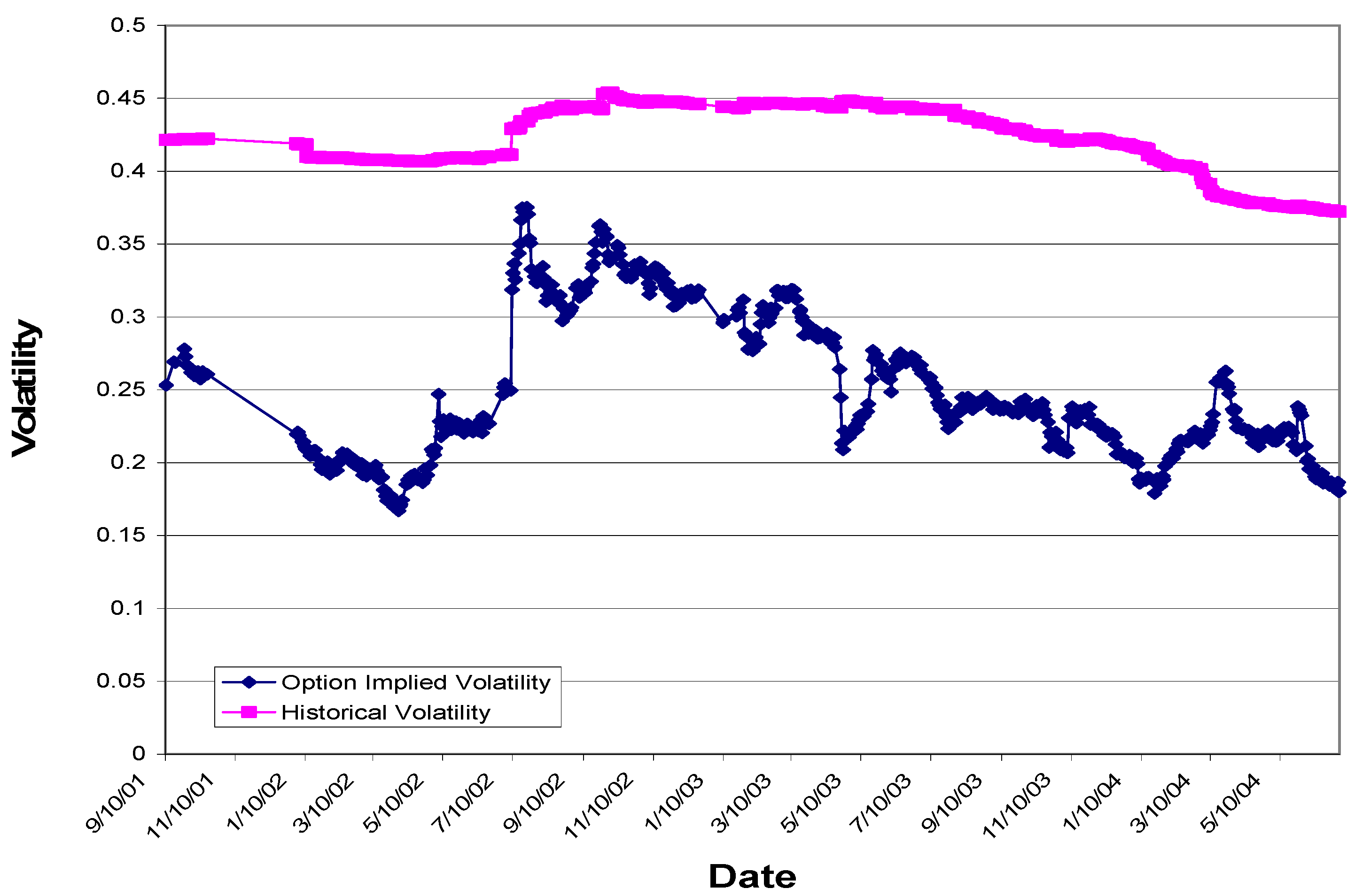
As demonstrated in Figure 3, historical volatility8 was a smooth curve while historical volatility had more sudden jumps, which confirmed the intuition that option-implied volatility incorporated information more promptly than historical volatility. The CDS spread computed with option-implied volatility therefore was able to send clearer trading signals than when it is computed with historical volatility.

The better fit of TS1 was also due to the special features of the CDS spread in relationship to volatility and stock price. First, the historical volatility was a very smooth curve—the difference between the historical volatilities between consecutive days was small. Second, the day-to-day changes of the CDS spread were small most of the time. The difference between the model spread of two consecutive days was caused by the different input to the CDS function. The only difference in input in this case was stock price and historical volatility. When historical volatilities were close to each other, the difference in model spread was mostly caused by the difference in stock prices. However, the stock price did not have a strong effect on the CDS spread, as demonstrated by the small magnitude of the partial derivative of the CDS spread over stock price. In a nutshell, the smoothness of both historical volatility and market realized CDS spread made TS1 fit better than TS2.

To provide an intuitive perspective, let us take a closer look at one of the trading opportunities that TS2 catches but TS1 misses for intuition. The stock price of Wyeth dropped on 9 July 2009 because of the concern that the Senate committee that oversees the U.S. Food and Drug Administration was likely to pass a compromise bill, sponsored by Senators John McCain, an Arizona Republican, and Charles Schumer, a New York Democrat, to tighten two loopholes in a 1984 law that let brand-name drug makers delay generic competition. The loophole allows brand-name drug makers like Wyeth to get a 30-month hold on approvals of generic versions of their drugs if they claim their patents have been infringed, which would stall the competition from generic drug manufacturers.

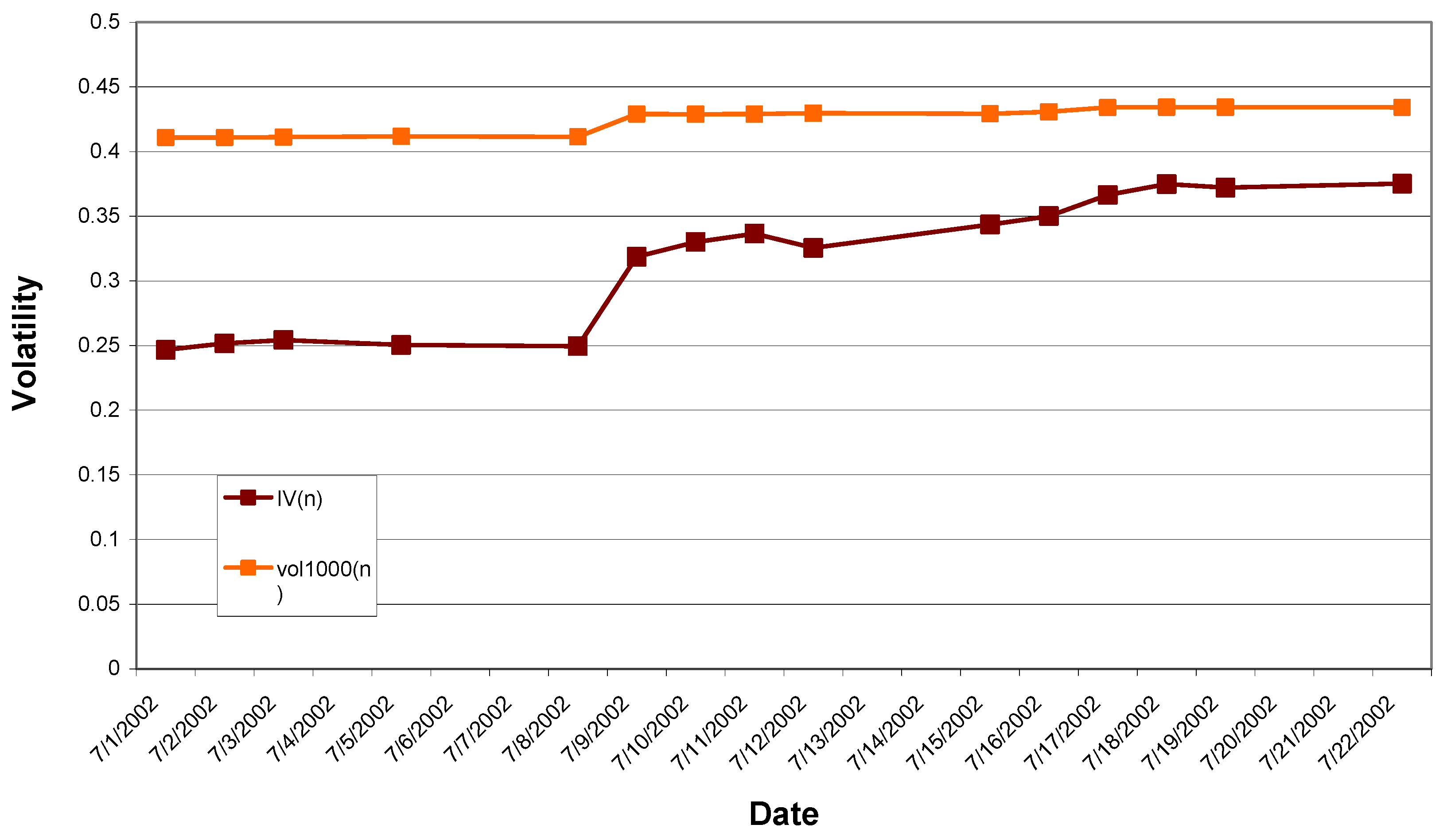
As demonstrated in Figure 4, on 8 July 2008, the market spread, TS1 modeled spread, and TS2 modeled spreads are all at a low level around 50 basis points. On 9 July, the market CDS spread increased substantially. TS2 soared upward, far above the market CDS spread, giving a strong signal that market CDS spread would increase further. The large difference between the TS2 and market CDS spreads sparked a trading signal. This trading signal turned out to be profitable—on 22 July when the TS2 spread and market CDS spread converged, the market CDS spread had more than tripled and the arbitrageur who used TS2 to trade would have profited. The TS1 spread, on the other hand, did not generate any trading signals and the arbitrageur who carried out TS1 would have missed the opportunity. The TS1 spread rose a bit higher than the market CDS spread on 9 July and then dropped below the market CDS spread until the trade initiated by TS2 liquidated.

Why did TS2 catch an opportunity while TS1 missed it? As demonstrated in Figure 5, option-implied volatility gave a much clearer signal than historical volatility on 9 July 2008. Both volatilities stayed flat before 9 July 2008, when option-implied volatility jumped much more than historical volatility. This is why the CDS spread computed with the option-implied volatility could send a clearer signal of trading opportunity. The interpretation of the different behavior between implied and historical volatility is, first, implied volatility reacts to information more promptly than historical volatility; second, implied volatility reacts to the information with larger movement, which might incorporate the time varying volatility premium as Cao, Yu, and Zhong [26] show.

We now compare the profitability of TS1 and TS2 at an index level. We use the same methodology as in Section 5.2.1 whereupon we compare TS1 and Yu [27]. The statistics of the comparison are presented in

Table 4. TS2 vs. TS1.

Grade	Measure of Profitability	Estimate	StdErr	t-stat	p-Value
Investment	Sharpe Ratio **	0.888	0.199	4.46	<0.0001
	Positive Months *	0.052	0.03	1.75	0.044
	Positive Trades	−0.0336	0.0292	−1.15	0.2572
	Mean of AER **	−0.248	0.03683	−6.72	<0.0001
	Skewness of AER **	221.926	15.557	14.18	<0.0001
	Converged Trades	0.00506	0.00584	0.87	0.2
	20% drawdown Trades **	−0.0041	0.0048	−2.78	0.004
Speculative	Sharpe Ratio *	0.308	0.217	1.42	0.0821
	Positive Months	0.01	0.06	0.16	0.44
	Positive Trades *	−0.17	0.1	−1.73	0.09
	Mean of AER **	−3.1749	0.708	−4.63	<0.0001
	Skewness of AER *	−35.876	19.0494	−1.89	0.0662
	Converged Trades **	−0.12	0.0189	−6.11	<0.0001
	20% drawdown Trades **	−0.0435	0.00606	−7.18	<0.0001

Items with ** have a confidence level of more than 99%. Items with a single * have a confidence level of more than 90%.

. TS2 outperforms TS1 in five measures of profitability while underperforming it in three measures, at a confidence level of at least 95%, implying that TS2 outperforms TS1 in general.

5.2.3. TS2 vs. Trading Strategy in Yu [27]

To make the analysis complete, we now compare TS2 and Yu [27].

Again, to provide an intuitive perspective, we compare TS2 and Yu [27] in the case of an individual firm, Wyeth. As Figure 6 demonstrates, TS2 had a much tighter fit than Yu [27]. Yu [27] persistently overestimated the market spread for an extended period from 30 August 2002 to 3 March 2004. In the middle of the period, the fit was far off. At $threshold=0.5$, Yu [27] initiated 395 trades, with an average AER at 0.3114%, while TS2 initiated only 74 trades, with an average AER at 1.6486%, 5 times that of Yu [27]. All the trades in TS2 converge while only 38% of the trades Yu [27] initiates converge.

We now compare the profitability of TS2 and Yu [27] at an index level. We use the same methodology as we compare TS1 and Yu [27]. The statistics of the comparison are presented in

Table 5. TS2 vs. Yu [27].

Grade	Measure of Profitability	Estimate	StdErr	t-stat	p-Value
Investment	Sharpe Ratio **	2.08	0.13	15.65	<0.0001
	Positive Months **	0.22	0.02	10.97	<0.0001
	Positive Trades **	0.26	0.0042	61.49	<0.0001
	Mean of AER **	0.11906	0.00317	38.01	<0.0001
	Skewness of AER	66.5142	61.955	1.07	0.2889
	Converged Trades **	0.91372	0.0131	69.79	<0.0001
	20% drawdown Trades **	−0.0041	0.00065	−6.34	<0.0001
Speculative	Sharpe Ratio **	1.25	0.08	15.48	<0.0001
	Positive Months **	0.088	0.0121	7.28	<0.0001
	Positive Trades **	0.135	0.0299	4.52	<0.0001
	Mean of AER **	1.24615	0.14065	8.85	<0.0001
	Skewness of AER **	345.112	10.8582	31.79	<0.0001
	Converged Trades **	0.80013	0.00783	102.75	<0.0001
	20% drawdown Trades **	−0.0469	0.00668	−7.01	<0.0001

Except for skewness of AER across trades in TS2, all the null hypotheses are rejected at confidence levels of at least 99.9%, implying that TS2 outperforms Yu [27] substantially. Items with ** have a confidence level of more than 99.99%.

.

TS2 improves upon Yu [27] in almost all measurements of profitability, except for the skewness of AER for investment grade index.

5.3. Profitability of TS2

Profitability of TS2 measured in the same statistics as in the previous section is presented in

Table 6. Risk and Return Characteristics of TS2.

Grade	Measure of Profitability	CI_lower	CI_upper	Estimate	t-value	p-value
Investment	Sharpe Ratio	2.1001	2.3135	2.20678	40.54	<0.0001
	Positive Months	0.7018	0.7443	0.72329	67.51	<0.0001
	Positive Trades	0.7813	0.7963	0.78896	208.08	<0.0001
	Mean of AER	0.12398	0.137314	0.130615	38.46	<0.0001
	Skewness of AER	309.2084	333.7663	321.5794	51.72	<0.0001
	Converged Trades	0.9767	0.9895	0.98322	302.53	<0.0001
	20% drawdown Trades	0	0	0	NA	0
Speculative	Sharpe Ratio	0.7324	0.6327	0.8319	14.44	<0.0001
	Positive Months	0.4789	0.551	0.51496	28.04	<0.0001
	Positive Trades	0.4828	0.6223	0.55257	15.54	<0.0001
	Mean of AER	0.798488	1.273136	1.035907	8.53	<0.0001
	Skewness of AER	80.74568	110.7771	95.76341	12.5	<0.0001
	Converged Trades	0.8466	0.916	0.88129	49.75	<0.0001
	20% drawdown Trades	0.00057	0.0315	0.01604	2.03	0.05

Step 1:

For every threshold h, simulate TS2 and compute Sharpe ratios SR_h.9 This step produces the series of SR_h, with h ranging from 0.5 to 1.5 in an increment of 0.025.

Step 2:

Run the following intercept-only regression and adjust for serial correlation in the error term with Newey-West adjustment:

$$\text{Regression}: \mathrm{S}{R}_h=\mathsf{\alpha }+{\mathsf{\epsilon }}_h , \text{with} E({\mathsf{\epsilon }}_h)=0 \text{for all} h.$$

The hypothesis test about intercept $\mathsf{\alpha }$: ${\mathrm{H}}_0:\mathsf{\alpha }=0vs.$ ${\mathrm{H}}_{\mathrm{a}}:\mathsf{\alpha }\ne 0$

Step 3:

Repeat Step 1 and Step 2 but replace Sharpe ratio with other measures of profitability, including the proportion of months with positive excess return, proportion of trades with positive excess, mean and skewness of the AERacross trades, proportion of trades that converges, and proportion of trades with a 20% drawdown10.

Table 6 reports the lower bound of the confidence interval, upper bound of the confidence interval, estimate, t-statistics, and p-value of multiple measures of profitability.

. It is found that the profitability of the investment grade index is impressive while the performance of the speculative grade index is modest.

5.4. Persistence of Profitability of TS2

5.4.1. Persistence against Systematic Risk

Is TS2 market neutral? This question is answered by regressing the monthly excess returns of TS2 indexes on eight risk factors that proxy a wide range of systematic risks. The t-value and p-value of the intercept and the factor loadings are listed in

Table 7. Market Neutrality of TS2.

Rating Grade	Risk Factor	Alpha		Factor Loading
		t-value	p-Value	t-Value	p-Vlaue
Investment	SMB	16	<0.0001	−0.66	0.52
	HML	14.19	<0.0001	1.1	0.276
	MKTRF	11.24	<0.0001	−0.11	0.9156
	MOM	15.78	<0.0001	−0.52	0.6075
	RSIND	16.65	<0.0001	−1.6	0.1171
	RINV	15.85	<0.0001	1.04	0.3026
	RSPEC	15.48	<0.0001	0.36	0.7186
	RARB	14.23	<0.0001	0.28	0.7817
Speculative	SMB	4.23	0.00005	1.11	0.2757
	HML	1.28	0.10415	2.14	0.0385
	MKTRF	7.06	<0.0001	1.34	0.1883
	MOM	5.07	<0.0001	−1.15	0.2566
	RSIND	1.45	0.07785	4.88	<0.0001
	RINV	1.31	0.09945	−1.5	0.1415
	RSPEC	1.06	0.14695	0.81	0.4224
	RARB	1.44	0.0785	0.63	0.535

Step 1:

For every threshold h, simulate TS2 and record the monthly return of the CSA index. This step produces 41 time series of CSA index monthly return R_h,t, with h ranging from 0.5 to 1.5, t indexes the months.

Step 2:

For h = 0.5, regress the time series of monthly return on the systematic risk factors.

Step 3:

Repeat Step 2 for all the other values of h. This step results in 41 coefficient estimate pairs $({\mathsf{\alpha }}_{h,SMB},{\mathsf{\beta }}_{h,SMB})$ with 41 different values of h, ranging from 0.5 to 1.5.

Step 4:

Run the following regression with auto correlation in the error term adjusted with Newey-West adjustment.

$$\text{Regression} 3: {\mathsf{\alpha }}_{h,SMB}={\mathsf{\alpha }}_{SMB}+{\mathsf{\epsilon }}_{h,SMB}, \text{with} E({\mathsf{\epsilon }}_{h,SMB})=0 \text{for all} h$$

Test the following Hypotheses:

$$\text{Null Hypothesis} 1: {\mathsf{\alpha }}_{SMB}=0 vs. \text{Alternative Hypothesis} 1: {\mathsf{\alpha }}_{SMB}>0$$

Step 5:

Repeat Step 4 but with ${\mathsf{\alpha }}_{h,SMB}$ replaced by ${\mathsf{\beta }}_{h,SMB}$, ${\mathsf{\alpha }}_{SMB}$ replaced by ${\mathsf{\beta }}_{SMB}$, and of course the notation of ${\mathsf{\epsilon }}_{h,SMB}$ needs to be changed too.

Test the following Hypotheses:

$$\text{Null Hypothesis} 2: {\mathsf{\beta }}_{SMB}=0 vs. \text{Alternative Hypothesis} 2: {\mathsf{\beta }}_{SMB}\ne 0$$

If Null Hypothesis 1 is rejected while Null Hypothesis 2 is not rejected, we conclude that CSA index return does not have loading of risk factor SMB.

If Null Hypothesis 2 is rejected, then we conclude that CSA index return does have loading of risk factor SMB.

Step 6:

Repeat Steps 4–5, but with SMB replaced by other risk factors.

As demonstrated in the table, for investment grade, Null Hypothesis 1 is rejected for all measures of profitability, and Null Hypothesis 2 is not rejected for any measures of profitability. Our conclusion is therefore, for investment grade obligors, TS2 does not have any loading of any of the risk factors. For speculative grade, the result is less clean.

.

As demonstrated in the table, for the investment grade index, none of the coefficients of the risk factors are statistically significant while all the intercepts are statistically significant.

The result for speculative grade is not as clean, which might be because the sample size of speculative grade obligors is small. Therefore, we may have less confidence on the test result for speculative grade obligors.

5.4.2. Persistence against Time

For a trading strategy, there is always worry that as the market matures with time, the profit of the trading strategy will dwindle. Does that happen to TS2? This question is answered by regression of the monthly excess returns of TS2 indexes on time.

The statistics of the tests are reported in

Table 8. Time Neutral of TS2.

	Alpha		Time Loading
Rating Grade	t-value	p-value	t-Value	p-Vlaue
Investment	4.19	0.0002	−0.91	0.3666
Speculative	0.78	0.4378	2.4	0.00107

Step 1:

For every threshold h, simulate TS2 and record the monthly return of the CSA index. This step produces 41 time series of CSA index monthly return R_h,t, with h ranging from 0.5 to 1.5, t indexes the months.

Step 2:

For $h=0.5$, perform the following time series regression, with auto correlation in the error term adjusted with Newey-West adjustment.

$$\text{Regression} 1: {\mathrm{R}}_{\mathrm{h},\mathrm{t}}={\mathsf{\alpha }}_h+{\mathsf{\beta }}_h\cdot t+{\mathsf{\epsilon }}_{h,t}, t \text{indexes the month}, \text{with} E({\mathsf{\epsilon }}_{h,t})=0, \text{for all} t.$$

Step 3:

Repeat Step 2 for all the other values of h. This step results in coefficient estimate pairs $({\mathsf{\alpha }}_h,{\mathsf{\beta }}_{\mathrm{h}})$ with 41 different values of h, ranging from 0.5 to 1.5.

Step 4:

Run the following regression with auto correlation in the error term adjusted with Newey-West adjustment.

$$\text{Regression} 2: {\mathsf{\alpha }}_h=\mathsf{\alpha }+{\mathsf{\epsilon }}_h \text{with} E({\mathsf{\epsilon }}_h)=0 \text{for all} h$$

Test the following Hypotheses:

$$\text{Null Hypothesis} 1: \mathsf{\alpha }=0 vs. \text{Alternative Hypothesis} 1: \mathsf{\alpha }>0$$

Step 5:

Repeat Step 4 but with ${\mathsf{\alpha }}_h$ replaced by ${\mathsf{\beta }}_h$, $\mathsf{\alpha }$ replaced by $\mathsf{\beta }$, and of course the notation of ${\mathsf{\epsilon }}_h$ needs to be changed too.

Test the following Hypotheses:

$$\text{Null Hypothesis} 2: \mathsf{\beta }=0 vs. \text{Alternative Hypothesis} 2: \mathsf{\beta }\ne 0.$$

If the estimate of $\mathsf{\beta }$ turns out to be positive, we test the following Hypotheses instead:

$$\text{Null Hypothesis} 3: \mathsf{\beta }=0 vs. \text{Alternative Hypothesis} 3: \mathsf{\beta }>0.$$

, and the description of the statistical procedure is described in the caption of the table.

For investment grade obligors, the coefficient of time is not statistically significant while the intercept is statistically significant; the answer is therefore “Yes”. For speculative grade obligors, the coefficient of time is actually statistically significantly positive, which means return of CSA grows with time. The intercept of the regression, however, is not statistically significant. The strange result in speculative grade might be due to the fact that the sample size of speculative grade obligors is very small in comparison with investment grade obligors; therefore, we may we may have less confidence in the test result for speculative grade obligors.

5.4.3. Picking up Nickels in front of a Steam Roller?

Some trading strategies pick up profits most of the time but suffer huge losses once in a while. Does TS2 suffer from the same symptom? This question is answered by studying the skewness of the AER across all trades of TS2.

Table 9. Skewness of AER across all trades in TS2.

Rating Grade	CI_Lower	CI_Upper	Estimate	t-value	p-value
Investment	19.4783	21.0253	20.2576	51.72	<0.0001
Speculative	5.0865	6.9783	6.032528	12.5	<0.0001

Step 1:

For every threshold h, simulate TS2 and compute the annualized excess return AER_h.11 This step produces the series of AER_h, with h ranging from 0.5 to 1.5 in an increment of 0.025.

Step 2:

Run the following intercept-only regression and adjust for serial correlation in the error term with Newey-West adjustment:

$$\text{Regression}: \mathrm{A}E{R}_h=\mathsf{\alpha }+{\mathsf{\epsilon }}_h , \text{with} E({\mathsf{\epsilon }}_h)=0 \text{for all} h$$

The hypothesis test about intercept $\mathsf{\alpha }$: ${\mathrm{H}}_0:\mathsf{\alpha }=0 vs.$ ${\mathrm{H}}_{\mathrm{a}}:\mathsf{\alpha }\ne 0$

Rejection of a hypothesis is interpreted as the skewness of AER is positive, and therefore, TS2 is not “picking up nickels in front of a steam roller”.

Table 9 reports the lower/upper bound of the confidence interval, estimate, t-statistics, and p-value of $\mathsf{\alpha }$.

The null hypothesis is rejected in both grades of CSA, interpreted as TS2 is not “picking up nickels in front of a steam roller.”

reports the statistics of the skewness. Formally, we test the following hypotheses:

H₀:

The skewness of the AER across all trades of TS2 is positive.

H_a:

The skewness of the AER across all trades of TS2 is zero.

It turns out that the skewness is greater than 0 with a confidence level of more than 99.9%. Therefore, the answer is “No”.

6. Conclusions and Discussion

This study shed new light on the credit spread puzzle by pointing out that the ability to accurately compute and dynamically update hedge ratios to facilitate a successful capital structure arbitrage is a distinctive strength of the Black-Scholes-Merton’s modeling paradigm, which could be utilized in credit risk models as well.

We provide economically significant evidence. Using an improved implementation, we showed that the model facilitated a successful capital structure arbitrage, which persistently produced substantial risk adjusted profit.

We do not suggest that our implementation is better than that of Huang and Huang [5]. In general, implementation should be tailored to the model and to the specific application. Moreover, even the same model should be implemented differently if different applications demand so. The way we implemented this particular model for this particular application does not serve as a general standard for the implementation of other models in the same paradigm. We do wish, of course, that individual elements of our implementation will be found helpful for fellow researchers.

We need to caution against the notion that the capital structure arbitrage in this study always works. Profitability of certain trading strategy is not the focus of this study. In general, trading strategy needs to be modified constantly in response to the changes in regulatory environment, market situation, etc. The regulatory environment of CDS trading has substantial changes over the years and there is surely no guarantee that a trading strategy will always work in spite of such changes.