Article

International Diversification Versus Domestic Diversification: Mean-Variance Portfolio Optimization and Stochastic Dominance Approaches

1
Faculty of Business and Economics, University of Sfax, Sfax 3018, Tunisia
2
Department of Statistics, The Chinese University of Hong Kong, Shatin, Hong Kong
3
Institute of Higher Business Studies, University of Sfax, Sfax, 3061, Tunisia
4
Department of Economics, Hong Kong Baptist University, Kowloon Tong, Hong Kong
*
Author to whom correspondence should be addressed.
J. Risk Financial Manag. 2014, 7(2), 45-66; https://doi.org/10.3390/jrfm7020045
Submission received: 15 October 2013 / Revised: 11 March 2014 / Accepted: 24 April 2014 / Published: 8 May 2014

Abstract

:
This paper applies the mean-variance portfolio optimization (PO) approach and the stochastic dominance (SD) test to examine preferences for international diversification versus domestic diversification from American investors’ viewpoints. Our PO results imply that the domestic diversification strategy dominates the international diversification strategy at a lower risk level and the reverse is true at a higher risk level. Our SD analysis shows that there is no arbitrage opportunity between international and domestic stock markets; domestically diversified portfolios with smaller risk dominate internationally diversified portfolios with larger risk and vice versa; and at the same risk level, there is no difference between the domestically and internationally diversified portfolios. Nonetheless, we cannot find any domestically diversified portfolios that stochastically dominate all internationally diversified portfolios, but we find some internationally diversified portfolios with small risk that dominate all the domestically diversified portfolios.

1. Introduction

Despite greater integration of international capital markets, investors continue to hold portfolios largely dominated by domestic assets. International investors’ preference for domestic stocks remains a subject of controversy, since many studies indicate that greater profits can be made by diversifying internationally. This paper applies the mean-variance portfolio optimization (PO) approach and the stochastic dominance (SD) test to examine preferences between domestic and international diversification strategies. We also examine whether there is an optimal investment strategy for American investors according to their risk level.
Our study is based on daily data consisting of the prices of the 30 highest capitalization US stocks and 20 international market indices from Latin American and Asian financial markets and the G6. The purpose of this paper is to identify empirically preferences for international diversification versus domestic diversification from American investors’ viewpoints. Consider the utility-maximizing investor who holds two diversified portfolios: an internationally diversified (IND) portfolio and a domestically diversified (DOD) portfolio. The objective is to rank investors’ preferences in regard to these two types of diversified portfolios to maximize investors’ expected wealth and/or expected utilities.
We first apply the PO technique to obtain efficient portfolios for both domestic and international diversification and study the preference for international versus domestic diversification for risk-averse investors. Our findings from applying the PO tool imply that the domestic diversification strategy is better for investors with a high risk level, while the international diversification strategy is the better choice for investors with a low risk level.
Since most of the portfolios including both DOD and IND portfolios are rejected to be normally distributed, the results drawn from the PO rule may be misleading. To circumvent this limitation, in this paper we also apply the SD test to examine preferences between the domestic and international diversification strategies, and we check whether there is an arbitrage opportunity between international and domestic stock markets, whether these markets are efficient, and whether investors are rational.
Our SD analysis shows that there is no arbitrage opportunity between international and domestic stock markets; domestically diversified portfolios with smaller risk dominate internationally diversified portfolios with larger risk and vice versa; and at the same risk level, there is no difference between the domestically and internationally diversified portfolios. These findings support arguments from those who claim that domestic diversification is better and those who claim that international diversification is better, as well as those who claim that there is no difference between domestic diversification and international diversification. Nevertheless, we find that domestically diversified portfolios with smaller risk dominate internationally diversified portfolios with larger risk and vice versa. This implies that the domestic diversification strategy with a lower risk level is preferred to the international diversification strategy with a higher risk level and vice versa. Nonetheless, we cannot find any domestically diversified portfolios that stochastically dominate all internationally diversified portfolios, but we find that internationally diversified portfolios with smaller risk dominate all the domestically diversified portfolios. This finding supports those who claim that international diversification is better. However, although our findings imply that international diversification is better at a low risk level, when the risk level is the same, there is no difference in the markets for domestically and internationally diversified portfolios.
The remainder of this paper is organized as follows. Section 2 contains a review of the related literature review. Section 3 discusses the data and the methodologies, including the PO portfolio optimization and the SD theory. Section 4 examines the empirical PO optimization results and the SD relationships between domestically and internationally diversified portfolios. The last section summarizes and concludes.

2. Literature Review

2.1. Portfolio Optimization

The classical mean-variance portfolio optimization (PO) model introduced by Markowitz [1] can be used to determine the asset allocation for a given capital investment. However, it has been demonstrated that the traditional estimated return for the Markowitz mean-variance (MV) optimization seriously departs from its theoretic optimal return [2]. To circumvent this limitation, Bai, Liu, and Wong [3] have developed new bootstrap-corrected estimations to estimate the optimal return and its asset allocation. They have proved that the bootstrap-corrected estimates are proportionally consistent with their theoretic counterparts. Bai, Liu, and Wong [4] extend their work by developing a bootstrap estimate for the optimal return of self-financing portfolios. Bai, Liu, and Wong [5] further develop some properties for the estimators. In addition, Leung, Ng, and Wong [6] further improve the estimation by deriving explicit formulas for the estimator of the optimal portfolio return and prove that their closed-form return estimator is consistent.
Most of the work on portfolio theory over the past decade has been based on the principle of utility maximization, where either the investor’s utility function is assumed to be a second-degree polynomial with a positive first derivative and a negative second derivative, or the probability functions are assumed to be normal [7]. Glen and Jorion [8] and others use the mean-variance (MV) analysis to investigate the benefits of international diversification based on a risk/return measurement. In spite of its popularity, the MV approach has been subject to serious criticism; see, for example, [9]. Wong [10] has shown that the mean-variance preference is equivalent to utility maximization if the assets being compared belong to the same location-scale family or the same linear combination of location-scale families.
To extend the MV model, Leung and Wong [11] develop a multiple Sharpe ratio test statistic to test the hypothesis of the equality of the multiple Sharpe ratios. Ma and Wong [12] establish some behavioral foundations for various types of VaR models, including VaR and conditional VaR, as measures of downside risk. In addition, Bai, Hui, Wong, and Zitikis [13] develop mean-variance-ratio statistics for comparing the performance of prospects after the effect of background risk has been mitigated. Bai, Phoon, Wang, and Wong [14] provide evidence that the mean-variance-ratio test is superior to the Sharpe ratio test by applying both tests to analyze the performance of commodity trading advisors.

2.2. Stochastic Dominance

To circumvent the limitation of the MV approach, academics suggest adopting the SD rules. The primary advantage of using the SD approach is that it provides a very general framework for assessing portfolio choice without the need for asset-pricing benchmarks. It does not need any assumption on the distribution of the assets being examined, and it satisfies the general utility function and takes into consideration all the distributional moments in the comparison [15]. The SD approach has been regarded as one of the most useful tools for ranking investment prospects (see, for example, [16]), since the ranking of assets has been shown to be equivalent to utility maximization for the preferences of risk averters and risk seekers [17].
The SD theory has been continually developed for more than half a century, and many SD comparisons have been carried out empirically. For example, Hodges and Yoder [18] use SD to test whether investors should prefer riskier securities as the investment horizon lengthens. Meyer, Li, and Rose [19] use the SD criteria to examine whether adding internationally based assets to a wholly domestic portfolio generates diversification benefits for an investor in New Zealand. Wong, Thompson, Wei, and Chow [20] offer an alternative view supporting the risk-based explanation of the momentum effect over the period 1965 to 2000. Lean, Smyth, and Wong [21] use the SD test to find evidence of weekday and monthly seasonality effects in some Asian markets. Gasbarro, Wong, and Zumwalt [22] apply the SD approach to find that over entire 1996–2003 period certain iShares dominate others. Fong, Lean, and Wong [23] apply the SD tests to conclude that the behavior of Internet stock prices is also consistent with the changing risk preferences of investors. In addition, Wong, Phoon, and Lean [24] find both first-order and higher-order SD relationships among the funds and conclude that investors would be better off investing in the first-order dominant funds to maximize their utility.
Recently, Abhyankar, Ho, and Zhao [25] find that value stocks stochastically dominate growth stocks only for the US, Canada, and Japan, while there are no significant SD relationships between these stocks for the UK, France, Germany, and Italy. Abid, Mroua, and Wong [26] find that the introduction of options improves the performance of unhedged portfolios, as does buying an in-the-money protective put. In addition, Lean, McAleer, and Wong [27] use the MV and SD approaches to reveal no evidence of any MV or SD relation-ships between oil spot prices and futures indices. Chan, De Peretti, Qiao, and Wong [28] adopt the SD and likelihood ratio test statistic approaches to conclude that neither the covered warrants nor the underlying shares stochastically dominate each other, which implies that the UK covered warrants market is efficient. Qiao, Clark, and Wong [29] apply the SD tests to find that the spot market dominates the futures market for risk averters, whereas futures dominate spot for risk seekers, implying that risk averters prefer to buy stocks, and risk seekers prefer long index futures.

2.3. International Versus Domestic Diversification Benefits

Many studies document the benefits of the diversification strategy. For example, Solnik [30] shows that substantial advantages in risk reduction can be attained through portfolio diversification in foreign securities as well as in domestic common stocks. Eun and Resnick [31] find potential gains from international diversification. Li, Sarkar, and Wang [32] reveal that the benefits of international diversification are substantial for US equity investors even though short selling is not allowed. Meyer and Rose [33] find that international diversi-fication can be advantageous and forms a means for managing crises in developed markets. Carrieri, Errunza, and Sarkissian [34] show that greater diversification gains can potentially be achieved if local industry investment is country specific and that investors should use both cross-country and cross-industry diversification as a way to improve portfolio performance.
In addition, Driessen and Laeven [35] document that the potential benefits from investing abroad remain substantial and the gains from international portfolio diversification are larger for countries with higher country risk. Chiou [36] finds that adding lower and upper weighting bounds reduces, but does not completely eliminate, the potential economic value of international investment. Eun, Lai, Roon, and Zhang [37] show that factor fund diversification strategies yield substantial improvements in portfolio efficiency beyond what can be achieved by traditional country market index diversification.
On the other hand, French and Poterba [38] show that most investors hold nearly all of their wealth in domestic assets. Tesar and Werner [39] report that domestic diversification was very evident in 1996. Lewis [40] shows that domestic stocks are a better hedge against home risks than foreign stocks. Kilka and Weber [41] show that actual equity portfolio holdings reveal a strong bias toward domestic stocks and conclude that this bias can be explained by the stock return expectations expressed in probability judgments. Oehler, Rummer, and Wendt [42] reveal that one of the phenomena documented in investment portfolios is the home-bias effect, since investors hold a higher-than-optimal portion of domestic assets. Antoniou, Olusi, and Paudyal [43] examine whether British investors need to diversify their portfolios internationally to gain performance benefits from international markets or whether they can obtain these benefits by mimicking the portfolios with domestically traded assets.

3. Data, Methodology and Hypotheses

3.1. Data

To analyze preferences between international and domestic diversification, in this paper we use daily arithmetic returns of the closing prices for the 30 highest capitalization US stocks and 20 international market indices from 1 January 1993 to 31 December 2012. The data are obtained from Datastream. We use the daily closing prices of the 30 highest capitalization US stocks (Table 1) to form several domestically diversified portfolios (DOD). To form the internationally diversified portfolios (IND), we use daily stock market indices from the G6 (the G7 excluding the US; that is, Canada, France, Germany, Italy, Japan, and the UK), and indices from Latin American and Asian countries. Latin American countries include Argentina, Brazil, and Mexico, while Asian countries include China, Hong Kong, India, Indonesia, South Korea, Malaysia, Pakistan, the Philippines, Sri Lanka, Taiwan, and Thailand. To avoid exchange rate bias, we express all indices and stock prices in US dollars [44].
Table 1. List of selected U.S. stocks.
1Apple (AAPL)16Citigroup (C)
2Exxon Mobil (XOM)17Merck (MRK)
3Microsoft (MSFT)18Verizon Communications (VZ)
4Johnson & Johnson (JNJ)19Cisco Systems (CSCO)
5General Electric (GE)20PepsiCo (PEP)
6Wal-Mart (WMT)21Schlumberger (SLB)
7Chevron (CVX)22Disney (DIS)
8Wells Fargo (WFC)23JPMorgan Chase (JPM)
9Procter & Gamble (PG)24Intel (INTC)
10IBM (IBM)25Home Depot (HD)
11Pfizer (PFE)26United Technologies (UTX)
12AT&T (T)27McDonald’s (MCD)
13Coca-Cola (KO)28Boeing (BA)
14Bank of America (BAC)29ConocoPhillips (COP)
15Oracle (ORCL)30Amgen (AMGN)
From the perspective of US investors, in this paper we adopt both PO and SD approaches to compare the performance of DOD and IND portfolios. We discuss the methodologies used in the paper in the following subsections. The selected stocks are listed by market capitalization.

3.2. Portfolio Optimization

We first adopt the classical portfolio optimization (PO) model [1] to determine the fraction xi (i = 1, …, n) of a given capital invested in asset iof portfolio P with its expected return, RP, being maximized subject to obtaining a pre-determined level of its variance Jrfm 07 00045 i008. More precisely, assuming that there are n assets, we denote Ri to be the expected return of asset i and σij to be the covariance of returns between asset i and asset j for i,j = 1,…, n. Given the required level of risk, Jrfm 07 00045 i008, for the portfolio, the classical PO model without short selling can be formulated as follows:
Jrfm 07 00045 i001
Bai, Liu, and Wong [3,4,5] have developed a new bootstrap-corrected estimation to estimate the optimal return and its asset allocation, while Leung, Ng, and Wong [6] derive the closed forms of the estimates. In this paper, we adopt their approaches to estimate the efficient portfolios for both international and domestic portfolios.

3.3. Stochastic Dominance Test

To overcome the limitations of the traditional MV criteria, the SD approach developed by Hadar and Russell [15], Hanoch and Levy [45], and others is one of the most useful tools for ranking investment prospects under uncertainty. Let X and Y represent DOD and IND portfolios with their cumulative distribution functions (CDFs), F and G, and their probability density functions (PDFs), f and g, respectively, defined on the common support of [a,b] with a < b. We define 1
Jrfm 07 00045 i002
For h = f,g; H = F,G; and j = 1,2,3. We call the integral Hj the jth order CDF.
The most commonly used SD rules are first-, second- and third-order SD, denoted as FSD, SSD and TSD, respectively. All investors are non-satiated (that is, prefer higher return to less) under FSD, non-satiated and risk-averse under SSD, and non-satiated, risk-averse, and possessing decreasing absolute risk aversion (DARA) under TSD. The SD rules [47] are:
X dominates Y by FSD (SSD, TSD), denoted by X ≽1 Y (X ≽2 Y, X ≽3 Y) if and only if F1(x) ≤ G1(x) (F2(x) ≤ G2(x), F3(x) ≤ G3(x)) for all possible returns x in [a,b]. In addition, if the strict inequality holds for at least one value of x, X dominates Y strictly by FSD (SSD, TSD), denoted by X ≻1 Y (X ≻2 Y, X ≻3 Y).
The theory of SD is important since it is related to utility maximization [48]. The existence of SD implies that risk-averse investors always obtain higher expected utilities when holding dominant assets than when holding dominated assets.2 Consequently, investors prefer dominant assets. We note that a hierarchical relationship exists in SD: FSD implies SSD, which, in turn, implies TSD. However, the converse is not true: the existence of SSD does not imply the existence of FSD. Likewise, the existence of TSD does not imply the existence of SSD or FSD. Thus, only the lowest dominance order of SD is reported if there is any.
We note that under certain regularity conditions,3 portfolio X stochastically dominates portfolio Y in the first order if and only if there is an arbitrage opportunity between X and Y, such that investors will increase their expected wealth, as well as their expected utility, if their investments are shifted from Y to X [24]. On the other hand, if FSD does not exist between X and Y, one could conclude that the markets are efficient and investors are rational [27].
There are two broad classes of SD tests: one is the minimum/maximum statistic [51,52], and the other is based on distribution values computed on a set of grid points (DD) [53]. Since the DD test is found to be one of the most powerful tests [54], we apply the DD test in our analysis.
For any two domestically and internationally diversified portfolios Y and Z with CDFs F and G, respectively, and for a grid of pre-selected points x1, x2… xk, the order-j DD statistic, Tj(x) (j = 1, 2, and 3), is:
Jrfm 07 00045 i003
where Jrfm 07 00045 i004 
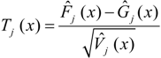
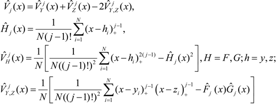
in which Fj and Gj are defined in (1), and (x)+ = {x,0}.
It is empirically impossible to test the null hypothesis for the full support of the distributions. We test the null hypothesis for a pre-designed finite numbers of values x. Specifically, the following hypotheses are tested:
  • H0 : Fj (xi) = Gj (xi), for all xi, i = 1,2,...,k;
  • HA : Fj (xi) ≠ Gj (xi) for some xi;
  • HA1 : Fj (xi) ≤ Gj (xi) for all xi, Fj (xi) < Gj (xi) for some xi;
  • HA2 : Fj (xi) ≥ Gj (xi) for all xi, Fj (xi) > Gj (xi) for some xi.
Bai, Li, Liu, and Wong [5] and Li, Bai, McAleer, and Wong [55] modify the DD test (modified DD test) with the following decision rules:
Jrfm 07 00045 i006
where Jrfm 07 00045 i007 
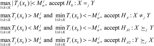
is the bootstrapped critical value of the j-order DD statistic. In this paper, we follow their recommendation to use simulated critical values in our analysis. We also follow their recommendation to use the maximum values of the test statistics to draw conclusions. However, since computing each grid point for the entire sample would entail a lot of computer time, we specify K equal-interval grid points {xk,k = 1,2,…,K} to cover the common support of random samples {Xi} and {Yi}, with K = 100 as recommended by Fong, Wong, and Lean [56], Gasbarro, Wong, and Zumwalt [22], and others. Simulation shows that the performance of the modified DD statistics is not sensitive to the number of grid points if the number of grid points is reasonably large, such as K = 100.
We note that in the above hypotheses, HA is set to be exclusive of both HA1 and HA2, which means that if either HA1 or HA2 is accepted, this does not mean that HA is accepted. Accepting either H0 or HA implies that there are no SD relationships and no arbitrage opportunity between these two diversified portfolios and neither of these two portfolios is preferred to the other. However, if HA1 or HA2 of order one is accepted, a particular DOD (IND) portfolio stochastically dominates another IND (DOD) portfolio at the first order. In this situation, there exists an arbitrage opportunity, and thus, non-satiated investors will be better off if they switch from the dominated portfolio to the dominant one. On the other hand, if HA1 or HA2 is accepted for order two or three, a particular DOD or IND stochastically dominates the other at the second or third order. In this situation, an arbitrage opportunity does not exist, and switching from one portfolio to another will only increase investors’ expected utilities, but not their expected wealth [24]. For j = 1,2, 3 the null hypothesis H0j states that DOD dominates the IND, F ≽j G, at order j, while the null hypothesis H Jrfm 07 00045 i005 states that the IND dominates the DOD portfolio, G ≽j F, at order j.

4. Empirical Results

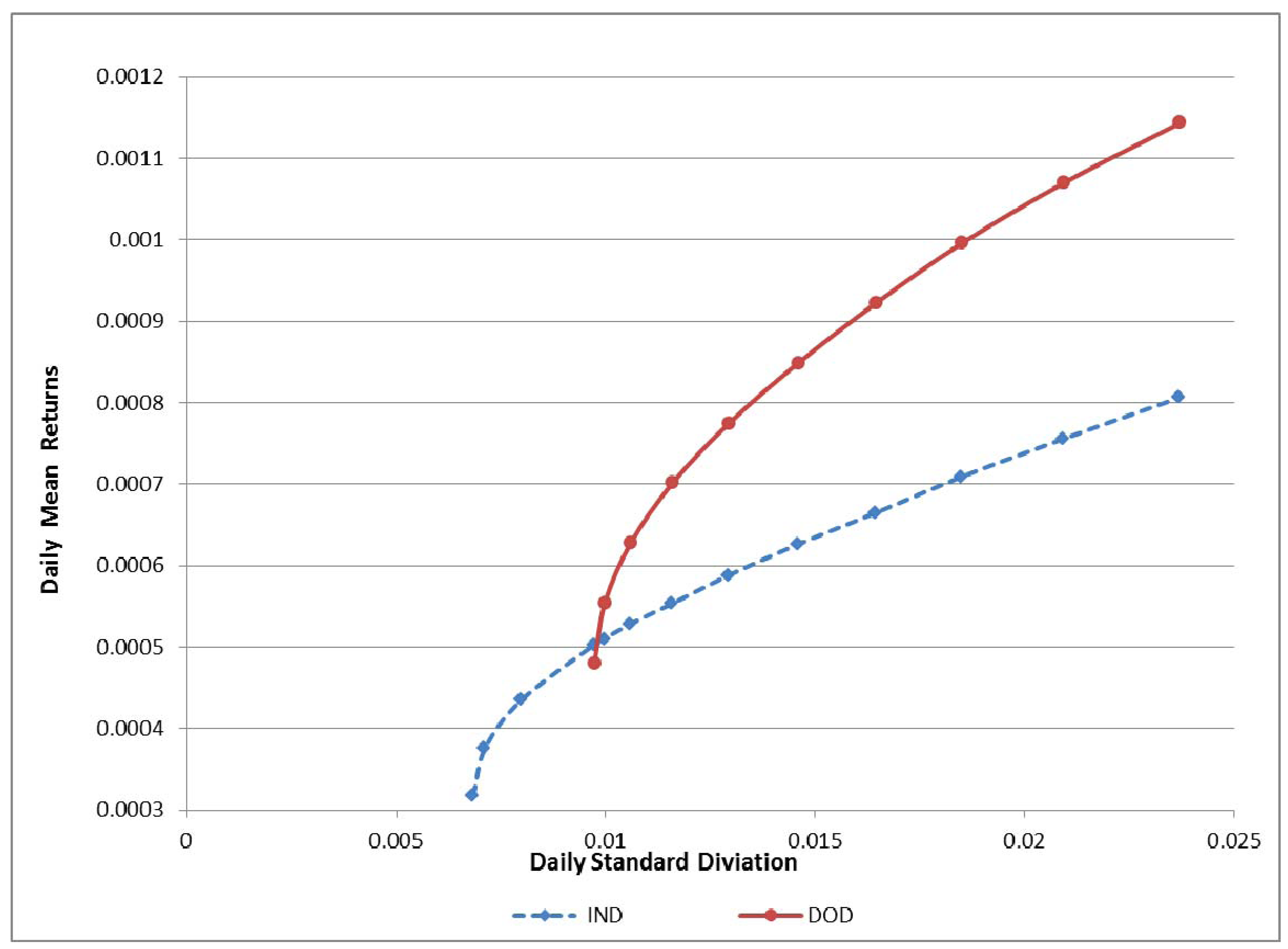
4.1. Portfolio Optimization

We first adopt the PO approach to examine the preferences of different DOD and IND portfolios for risk-averse investors. From the MV efficient portfolios derived, we construct the efficient MV frontiers for both IND and DOD strategies and display them in Figure 1. By doing so, one could construct various efficient sets, which, in turn, enable us to examine the performance of various diversification strategies for different levels of risk and return. We construct the 10 DOD and 13 IND portfolios as follows: (1) we start from the minimum risk point of the efficient frontier of the DOD portfolios and roughly divide them into 10 equal parts in terms of risk; (2) we compute the 10 points on the efficient frontiers of both the DOD and the IND portfolios using the same risk obtained in (1); (3) we compute 2 extra points on the efficient frontiers of the IND portfolios using the same distance of risk obtained in (1) leading to the minimum risk point of the IND; and (4) we include the minimum risk point of the IND.
Figure 1. Mean-variance (MV) efficient frontiers of international and domestic diversification strategies.
Jrfm 07 00045 g001
Note: IND is the efficient frontier of internationally diversified portfolios and DOD is the efficient frontiers of domestically diversified portoflios.
We first summarize in Table 2 and Table 3 the descriptive statistics of all 13 DOD and 10 IND portfolios, including the mean, standard deviation, coefficient of variation (CV), skewness, and kurtosis coefficients. From Table 2, we find that the daily mean return (standard deviation) of the DOD and IND portfolios varies from 0.00048 to 0.00114 (0.00973 to 0.02371) and from 0.00032 to 0.00081 (0.00684 to 0.02371), respectively. In general, DOD portfolios generate higher risk than IND portfolios. In addition, as shown in Table 3, the means and standard deviations vary widely across diversified portfolios. For example, DOD10 and IND13 possess the two largest daily mean returns (0.00114 and 0.00081) and the two largest standard deviations (0.02371 and 0.02371), while DOD1 and IND1 exhibit the two smallest mean returns (0.00048 and 0.00032) and the two smallest standard deviations (0.00973 and 0.000684). Regarding the coefficient of variation (CV), DOD 4 obtains the smallest value (16.53), while IND13 obtains the highest values (29.39). In addition, we show that, in general, DOD portfolios obtain smaller values than their IND counterparts. In particular, the values of the CV of DOD2 to DOD7 are smaller than those of any IND portfolio, while the values of the CV of IND1 and IND7–IND13 are bigger than those of any DOD portfolio.
We turn now to comparing the efficient frontiers of the DOD and IND from Figure 1. Since the efficient frontiers of the DOD and IND cross, applying the MV optimization rule to different efficient frontiers leads us to conclude that the DOD and IND do not dominate each other in the entire risk-return range. To be more specific, by adopting the MV optimization approach, we observe from Figure 1 that for any risk level less than 1%, the IND strategy clearly dominates the DOD strategy, but the dominance relationship is reversed for any risk level greater than 1%. This implies that the question of diversifying internationally or domestically would not have a unique answer for US investors and the answer would depend on what level of risk they want to take and what level of return they would like to get. If investors are willing to accept a risk level above 1%, the DOD strategy is a better choice. On the other hand, if they are only willing to accept a risk level up to 1%, the IND strategy is the better choice for them.
Table 2. Summary statistics of the domestic MV efficient diversified portfolios.
Mean (µ)Std Dev (σ)CV (σ/µ)SkewnessKurtosis
DOD10.000480.0097320.260.190969.21767
DOD20.000550.0099718.010.152128.61416
DOD30.000630.0105916.880.106307.39123
DOD40.000700.0115916.530.076936.09004
DOD50.000770.0129516.720.062305.29170
DOD60.000850.0145917.190.035724.87478
DOD70.000920.0164517.840.024824.73178
DOD80.000100.0185118.580.038474.94001
DOD90.001070.0209319.570.031145.46898
DOD100.001140.0237120.730.020055.95474
Note: This table reports the summary statistics of the 10 domestic MV efficient diversified (DOD) portfolios, DOD1 to DOD10, including mean (µ), standard deviation (σ), the coefficient of variation (σ/µ), skewness, and kurtosis coefficients. The construction of DOD1 to DOD10 is described in Section 4.1.
Table 3. Summary statistics of the international MV efficient diversified portfolios.
Mean (µ)Std Dev (σ)CV (σ/µ)SkewnessKurtosis
IND10.000320.0068421.53−0.210075.04703
IND20.000380.0071218.92−0.187264.45829
IND30.000440.0079918.36−0.159113.76602
IND40.000500.0097319.34−0.123443.49837
IND50.000510.0099719.54−0.119183.54673
IND60.000520.0105920.04−0.106543.72651
IND70.000550.0115920.93−0.058063.88917
IND80.000590.0129422.00−0.048534.43614
IND90.000630.0145923.30−0.006874.79284
IND100.000660.0164524.740.015995.32968
IND110.000710.018512609.170.075455.83010
IND120.000760.0209327.690.108626.26873
IND130.000810.0237129.390.136476.54289
Note: This table reports the summary statistics of the 13 international MV efficient diversified (IND) portfolios, IND1 to IND13, including mean (µ), standard deviation (σ), the coefficient of variation (σ/µ), skewness, and kurtosis coefficients. The construction of IND1 to IND13 is described in Section 4.1.

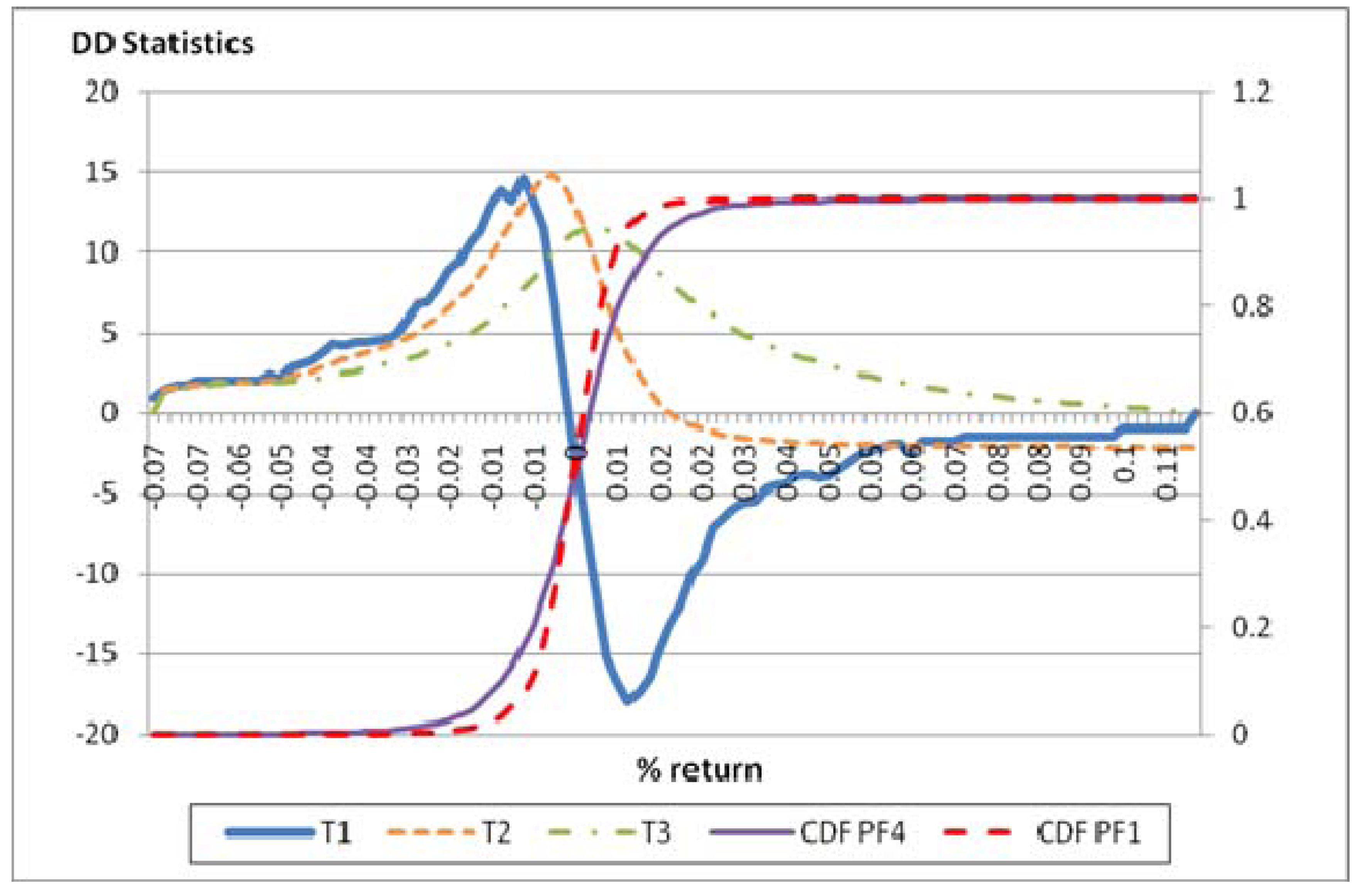
4.2. Stochastic Dominance

The results from the PO approach discussed in the previous subsection show that the international diversification strategy dominates the domestic diversification strategy in a risk-return range but the dominance relationship is reversed in another risk-return range. In addition, from Table 2 and Table 3, we find that the normality hypothesis is rejected for most of the portfolios. This suggests that the results from the PO rule may be misleading. To circumvent this limitation, we use the SD approach and adopt the DD (2000) test to examine investors’ preferences between the DOD and the IND strategies. We summarize the results in Table 4 and Table 5. For example, if we report DOD (F) SSD IND (G), this means that DOD stochastically dominates IND strictly in the sense of second-order SD, and denoted by F ≻ 2G or F SSD dominates G. On the other hand, ND refers to no dominance between F and G. This means that either it H0:F = G or HA:FG is accepted. Readers may refer to the notes in Table 4 and Table 5 for more information on other notations.
To get a better picture of the results of the DD test, we plot the DD test and corresponding CDFs for each DOD and IND for two pairs of observations in Figure 2 and Figure 3 for illustration. The first pair is the DOD4 and IND1 portfolios, and the second pair is the DOD3 and IND13 portfolios. From Figure 2 (3), we find that the empirical distribution functions of DOD 4 and IND1 (DOD3 and IND13) cross, implying that it is very likely that there is no first-order SD between the DOD4 and IND1 (DOD3 and IND13) portfolios. The result of the T1 statistic being significantly positive and negative in both figures confirms the absence of the FSD relationship. However, Figure 2 (3) reveals that the T2 and T3 statistics are significantly positive (negative), showing that the IND1 (DOD3) SSD and TSD-dominates DOD4 (IND13). Since the hierarchical relationship exists in SD that SSD implies TSD, we report only SSD if both SSD and TSD relationships are found. The results of the SD relationship between the IND and DOD portfolios are reported in Table 4 and Table 5.
Figure 2. Plot of the cumulative distribution function (CDF) of the daily returns of the fourth domestic diversified portfolio (DOD 4) and the first international diversified portfolio (IND 1) and their DD statistics.
Jrfm 07 00045 g002
Figure 3. Plot of the CDF of the daily returns of the third domestic diversified portfolio (DOD3) and the 13 international diversified portfolios (IND13) and their DD statistics.
Jrfm 07 00045 g003
Table 4. Stochastic dominance test between domestically and internationally diversified portfolios.
PortfoliosIND1IND2IND3IND4IND5IND6IND7IND8IND9IND10IND11IND12IND13SSD
DOD1 NDNDSSDSSDSSDSSDSSDSSDSSDSSD8
DOD2 NDNDSSDSSDSSDSSDSSDSSDSSDSSD8
DOD3 NDNDNDSSDSSDSSDSSDSSDSSDSSD7
DOD4 NDNDSSDSSDSSDSSDSSDSSD6
DOD5 NDSSDSSDSSDSSDSSD5
DOD6 NDSSDSSDSSDSSD4
DOD7 NDSSDSSDSSD3
DOD8 NDSSDSSD2
DOD9 NDSSD1
DOD10 ND0
SSD0000023456789
Note: This table reports the stochastic dominance results to test whether domestically diversified (DOD) portfolios strictly dominate internationally diversified (IND) portfolios in the sense of the j order stochastic dominance for j = 1, 2, 3. The test is based on DD test statistics (refer to Equation 3) significance for the first three SD orders (FSD, SSD, and TSD). The results in this table are read on a row-versus-column basis. For example, the cell in the first row and the 6th column tells us that DOD1 stochastically dominates IND6 in the sense of SSD and TSD. FSD, SSD, TSD, and ND stand for the first-, second-, third-order stochastic dominance, and no stochastic dominance, respectively. Indifference relationships between DOD and IND are presented in the shaded areas. The entries in the last column (row) show the numbers of total SSD dominance for the corresponding row (column).
Table 5. Stochastic dominance test between global internationally and domestically diversified portfolios.
PortfoliosDOD1DOD2DOD3DOD4DOD5DOD6DOD7DOD8DOD9DOD10SSDTSDTotal
IND1SSDSSDSSDSSDSSDSSDTSDSSDTSDTSD7310
IND2SSDSSDSSDSSDSSDSSDSSDSSDSSDSSD10010
IND3SSDSSDSSDSSDSSDSSDSSDSSDSSDSSD10010
IND4NDNDNDSSDSSDSSDSSDSSDSSDSSD707
IND5NDNDNDSSDSSDSSDSSDSSDSSDSSD707
IND6 NDNDSSDSSDSSDSSDSSDSSD606
IND7 NDSSDSSDSSDSSDSSDSSD606
IND8 NDSSDSSDSSDSSDSSD505
IND9 NDSSDSSDSSDSSD404
IND10 NDSSDSSDSSD303
IND11 NDSSDSSD202
IND12 NDSSD101
IND13 ND000
SSD3335788101011
TSD0000001011
Total3335789101112
Note: This table reports the stochastic dominance results to test whether domestically diversified (DOD) portfolios strictly dominate internationally diversified (IND) portfolios in the sense of the j order stochastic dominance for j =1,2,3. The test is based on DD test statistics (refer to equation 3) significance for the first three SD orders (FSD, SSD, and TSD). The results in this table are read on a row-versus-column basis. For example, the cell in the first row and the second column tells us that IND1 stochastically dominates DOD2 in the sense of SSD and TSD. FSD, SSD, TSD, and ND stand for the first-, second-, third-order stochastic dominance, and no stochastic dominance, respectively. Indifference relationships between DOD and IND are presented in the shaded areas. The entries in the third [second] to last column (row) show the numbers of total SSD [TSD] dominance for the corresponding row (column) and the entries in the last column (row) show the numbers of total [SSD+TSD] dominance for the corresponding row (column).
From Table 4, we find that some domestically diversified portfolios SSD-dominate some internationally diversified portfolios in the sense of SSD. More precisely, we find that 44 (33.8 percent) of the DOD portfolios SSD-dominate some IND portfolios, implying that risk-averse US investors will prefer 33.8 percent of DOD portfolios relative to the corresponding IND portfolios. This, in turn, supports the argument from those who claim that domestic diversification is better.
On the other hand, from Table 5, we observe that some internationally diversified portfolios SSD- and TSD-dominate some domestically diversified portfolios. More precisely, we find that 68 (52.3 percent) IND portfolios SSD-dominate DOD portfolios, implying that second-order risk-averse US investors will prefer 52.3 percent of IND portfolios relative to their corresponding DOD portfolios. A similar conclusion can be drawn for the third-order SD dominance from IND to DOD. This supports the argument from those who claim that international diversification is better.
In addition, from Table 4 and Table 5, we find some domestically diversified portfolios and internationally diversified portfolios that do not dominate each other, supporting the argument that IND and DOD do not dominate each other. More precisely, from Table 4 and Table 5, we find that 15 (11.5 percent) of the DOD and IND do not dominate each other, implying that in 11.5 percent of cases, US investors are indifferent between investing in DOD and IND. This, in turn, supports the argument that there is no difference between domestic diversification and international diversification.
Moreover, from Table 4, we find that DOD portfolios with smaller risk stochastically dominate IND portfolios with larger risk. Similarly, from Table 5, we find that IND portfolios with smaller risk stochastically dominate DOD portfolios with larger risk. These findings lead us conclude that the domestic diversification strategy with a lower risk level stochastically dominates the international diversification strategy with a higher risk level, which, in turn, supports those who advocate domestic diversification. On the other hand, for a low risk level in foreign markets, an international diversification strategy stochastically dominates a domestic diversification strategy, which, in turn, supports those who favor international diversification. Nonetheless, we find that DOD1 and DOD2 are the “best” portfolios among all the DOD portfolios, since they SSD-dominate 8 IND portfolios (IND6–IND13). However, they cannot dominate the other five portfolios IND (IND1–IND5). Thus, we cannot find any domestic portfolio that dominates all international portfolios. However, Table 5 shows that IND1 to IND 3 SSD/TSD-dominate all the DOD portfolios. Thus, we can claim that IND1–IND 3 are the best choices; this, in turn, supports those who claim that international diversification is better.
Moreover, from Table 4, we find that DOD portfolios with smaller risk stochastically dominate IND portfolios with larger risk. Similarly, from Table 5, we find that IND portfolios with smaller risk stochastically dominate DOD portfolios with larger risk. These findings lead us conclude that the domestic diversification strategy with a lower risk level stochastically dominates the international diversification strategy with a higher risk level, which, in turn, supports those who advocate domestic diversification. On the other hand, for a low risk level in foreign markets, an international diversification strategy stochastically dominates a domestic diversification strategy, which, in turn, supports those who favor international diversification. Nonetheless, we find that DOD1 and DOD2 are the “best” portfolios among all the DOD portfolios, since they SSD-dominate 8 IND portfolios (IND6–IND13). However, they cannot dominate the other five portfolios IND (IND1–IND5). Thus, we cannot find any domestic portfolio that dominates all international portfolios. However, Table 5 shows that IND1 to IND3 SSD/TSD-dominate all the DOD portfolios. Thus, we can claim that IND1–IND3 are the best choices; this, in turn, supports those who claim that international diversification is better.
Now, we use two examples displayed in Table 6 and Table 7 to illustrate how to draw the two different dominance conclusions displayed in Table 4 and Table 5. The first example shown in Table 6 exhibits the first three orders of DD statistics between DOD1 and IND2. From the table, we find that 18.3 percent (20.8 percent) of the first-order DD statistic T1 is significantly positive (negative); thus, the results lead us to reject the hypothesis that DOD1 FSD-dominates IND2 or vice versa. The table also shows that 39.9 percent of the second-order DD statistic T2 is significantly positive and none of it is significantly negative. This implies that IND 2 SSD-dominates DOD1. Similarly, we find that 27.9 percent of the third-order DD statistic T3 is significantly positive and none of it is significantly negative. This shows that IND2 TSD-dominates DOD1. Finally, we illustrate the second example in Table 7. From the table, we find that no percentage of T1, T2 and T3 is significantly positive or negative. This implies that DOD1 and IND5 do not dominate each other in the sense of the first-, second-, and third-order SD.
Table 6. The results of the stochastic dominance (SD) statistics for the first domestic diversified portfolio (DOD1) and the second international diversified portfolios (IND2).
FSD
T1 > 0T1 < 0
Total (%)18.320.8
Positive Domain (%)18.30
Negative Domain (%)020.8
Max (|Tj|)8.319.92
SSD
T2 > 0T2 < 0
Total (%)39.90
Positive Domain (%)39.90
Negative Domain (%)00
Max (|Tj|)8.530.63
TSD
T3 > 0T3 < 0
Total (%)27.90
Positive Domain (%)27.90
Negative Domain (%)00
Max (|Tj|)6.97NA
Notes: Readers may refer to equation (3) for the formula of Tj for j=1,2,3 with F = DOD1 and G = IND2. The period is from 1 January 1993 to 31 December 2012.
Table 7. The results of the stochastic dominance (SD) statistics for the first domestic diversified portfolio (DOD1) and the fifth international diversified portfolios (IND5).
FSD
T1 > 0T1 < 0
Total (%)00
Positive Domain (%)00
Negative Domain (%)00
Max (|Tj|)2.802.99
SSD
T2 > 0T2 < 0
Total (%)00
Positive Domain (%)00
Negative Domain (%)00
Max (|Tj|)1.882.12
TSD
T3 > 0T3 < 0
Total (%)00
Positive Domain (%)00
Negative Domain (%)00
Max (|Tj|)1.751.21

5. Conclusions

In this paper, we compare the performance of the efficient domestically and internationally diversified portfolios by applying both the mean-variance portfolio optimization (PO) and the stochastic dominance (SD) approaches to analyze the Latin American and Asian financial markets and the G6 from 1 January 1993 to 31 December 2012. Comparing the MV efficient frontiers, we find that one efficient strategy could dominate the other over a range of risk and return but the dominance relationship could be reversed over another range of risk and return. Our PO results show that for investors who are willing to accept a higher risk level, a domestic diversification strategy is better for them. On the other hand, if they are only willing to accept a lower risk level, an international diversification strategy is a better choice.
Since the normality hypothesis is rejected for most of the portfolios, the results drawn from the PO rule may be misleading. To circumvent this limitation, we use the Davidson and Duclos test to examine investors’ preferences between the domestic and international diversification strategies. Our SD analysis shows that there is no arbitrage opportunity between international and domestic stock markets. We find that some domestically diversified portfolios SSD-dominate some internationally diversified portfolios, supporting those who claim that domestic diversification is better. On the other hand, we observe that some internationally diversified portfolios SSD- and TSD-dominate some domestically diversified portfolios, supporting the argument of those who claim that international diversification is better. In addition, we find that some domestically and internationally diversified portfolios do not dominate each other, supporting the argument that there is no difference between domestic and international diversification. Nevertheless, we find that domestically diversified portfolios with smaller risk SSD-dominate internationally diversified portfolios with larger risk and vice versa. This implies that for a lower risk level in domestic markets, the domestic diversification strategy stochastically dominates the international diversification strategy with higher risk, which, in turn, supports the finding that there are benefits from domestic diversification. On the other hand, for a low risk level in foreign markets, an international diversification strategy stochastically dominates a domestic diversification strategy with higher risk, which, in turn, supports the finding that there are benefits from international diversification. Nonetheless, we cannot find any domestically diversified portfolio that stochastically dominates all internationally diversified portfolios but we find that the internationally diversified portfolios with a risk smaller than that of any domestically diversified portfolio SSD- or TSD-dominate all the domestically diversified portfolios. This supports the claim that international diversification is better. However, although our findings imply that international diversification is better at a lower risk level, the markets for the domestic and international diversification strategies are efficient when they have the same risk level.
One may argue that our findings could fit any argument. So what can investors learn from our findings? Our answer is that yes, it is true that our analysis provides grounds to support any argument. However, all the arguments are true only under some conditions. We summarize our main findings as follows: (1) risk-averse investors are indifferent between the domestic and international diversification strategies if both strategies have the same risk; (2) when comparing the domestically diversified portfolios with lower risk and the internationally diversified portfolios with higher risk, risk averters would prefer to invest in the domestically diversified portfolios; (3) when comparing the internationally diversified portfolios with lower risk with the domestically diversified portfolios with higher risk, risk averters would prefer to invest in the internationally diversified portfolios; and (4) the risk of some internationally diversified portfolios is smaller than that of all domestically diversified portfolios, implying that risk averters will prefer only international diversification if they can invest in these smaller-risk internationally diversified portfolios.
Finally, one may wonder whether there is any contradiction for our PO and SD findings because from our PO finding, we conclude that the domestic diversification strategy is better for investors with a higher risk level, while the international diversification strategy is the better choice for investors with a lower risk level. This seems to contradict the SD findings of (1) to (4) above. We note that there is no contradiction. Our SD finding is the refinement of our PO finding. Our PO finding shows that for a higher risk, the mean of the DOD is higher than that of the IND, and thus, the results from our PO analysis conclude that the domestic diversification strategy is better. However, our SD analysis shows that this is not true. Our SD analysis shows that for a higher risk, the mean of the DOD is higher than that of the IND, but the DOD does not stochastically dominate any IND portfolio, and thus, investors in these 2 markets are indifferent between the IND and DOD portfolios with the same risk.
An extension could include examining the preferences of other types of investors, such as risk seekers [48] and investors with S-shaped and reverse S-shaped utility functions; see, for example, [46,57,58]. Extensions could also include applying behavioral finance methods [59,60,61] to examine the behavior of different investors when deciding whether to invest domestically or internationally.

Acknowledgments

The research is partially supported by the University of Sfax, The Chinese University of Hong Kong, Hong Kong Baptist University, and the Research Grants Council (RGC) of Hong Kong.

Author Contributions

All authors made substantial contributions for this paper.

Conflicts of Interest

The authors declare no conflict of interest.

References

  1. H. Markowitz. “Portfolio selection.” J. Financ. 7 (1952): 77–91. [Google Scholar]
  2. R.O. Michaud. “The Markowitz optimization enigma: Is “optimized” optimal? ” Financ. Anal. J. 45 (1989): 31–42. [Google Scholar] [CrossRef]
  3. Z.D. Bai, H.X. Liu, and W.K. Wong. “Enhancement of the applicability of Markowitz’s portfolio optimization by utilizing random matrix theory.” Math. Financ. 19 (2009): 639–667. [Google Scholar] [CrossRef]
  4. Z.D. Bai, H.X. Liu, and W.K. Wong. “On the Markowitz mean-variance analysis of self-financing portfolios.” Risk Decis. Anal. 1 (2009): 35–42. [Google Scholar]
  5. Z.D. Bai, H. Li, H.X. Liu, and W.K. Wong. “Test statistics for prospect and Markowitz stochastic dominances with applications.” Econom. J. 14 (2011): 278–303. [Google Scholar] [CrossRef]
  6. P.L. Leung, H.Y. Ng, and W.K. Wong. “An improved estimation to make Markowitz’s portfolio optimization theory practically useful and users friendly.” Eur. J. Oper. Res. 222 (2012): 85–95. [Google Scholar] [CrossRef]
  7. R.B. Porter, and J.E. Gaumnitz. “Stochastic dominance vs. mean-variance portfolio analysis: An empirical evaluation.” Am. Econ. Rev. 62 (1972): 438–446. [Google Scholar]
  8. J. Glen, and P. Jorion. “Currency hedging for international portfolios.” J. Financ. 48 (1993): 1865–1886. [Google Scholar] [CrossRef]
  9. S. Ross. “Some stronger measures of risk aversion in the small and the large with applications.” Econometrica 49 (1981): 621–638. [Google Scholar] [CrossRef]
  10. W.K. Wong. “Stochastic dominance and mean-variance measures of profit and loss for business planning and investment.” Eur. J. Oper. Res. 182 (2007): 829–843. [Google Scholar] [CrossRef]
  11. P.L. Leung, and W.K. Wong. “On testing the equality of the multiple Sharpe ratios, with application on the evaluation of iShares.” J. Risk 10 (2008): 1–16. [Google Scholar]
  12. C. Ma, and W.K. Wong. “Stochastic dominance and risk measure: A decision-theoretic foundation for VaR and C-VaR.” Eur. J. Oper. Res. 207 (2010): 927–935. [Google Scholar] [CrossRef]
  13. Z.D. Bai, K.F. Phoon, K.Y. Wang, and W.K. Wong. “The performance of commodity trading advisors: A mean-variance-ratio test approach.” N. Am. J. Econ. Financ. 25 (2013): 188–201. [Google Scholar] [CrossRef]
  14. Z.D. Bai, Y.C. Hui, W.K. Wong, and R. Zitikis. “Evaluating prospect performance: Making a case for a non-asymptotic UMPU test.” J. Financ. Econ. 10 (2012): 703–732. [Google Scholar]
  15. J. Hadar, and S. Russel. “Rules for ordering uncertain prospects.” Am. Econ. Rev. 59 (1969): 25–34. [Google Scholar]
  16. H. Levy. “Stochastic dominance and expected utility: Survey and analysis.” Manag. Sci. 38 (1992): 555–593. [Google Scholar] [CrossRef]
  17. C.K. Li, and W.K. Wong. “Extension of stochastic dominance theory to random variables RAIRO.” Rech. Opér. 33 (1999): 509–524. [Google Scholar]
  18. C. Hodges, and J. Yoder. “Time diversification and security preferences: A stochastic dominance analysis.” Rev. Quant. Financ. Account. 7 (1996): 289–298. [Google Scholar] [CrossRef]
  19. O.T. Meyer, X.M. Li, and C.L. Rose. “Comparing mean variance tests with stochastic dominance tests when assessing international portfolio diversification benefits.” Financ. Serv. Rev. 14 (2005): 149–168. [Google Scholar]
  20. W.K. Wong, H.E. Thompson, S. Wei, and Y.F. Chow. “Do winners perform better than losers? A stochastic dominance approach.” Adv. Quant. Anal. Financ. Account. 4 (2006): 219–254. [Google Scholar] [CrossRef]
  21. H.H. Lean, R. Smyth, and W.K. Wong. “Revisiting calendar anomalies in Asian stock markets using a stochastic dominance approach.” J. Multinatl. Financ. Manag. 17 (2007): 125–141. [Google Scholar] [CrossRef]
  22. D. Gasbarro, W.K. Wong, and J.K. Zumwalt. “Stochastic dominance analysis of iShares.” Eur. J. Financ. 13 (2007): 89–101. [Google Scholar] [CrossRef]
  23. W.M. Fong, W.K. Wong, and H.H. Lean. “Stochastic dominance and the rationality of the momentum effect across markets.” J. Financ. Mark. 8 (2005): 89–109. [Google Scholar]
  24. W.K. Wong, K.F. Phoon, and H.H. Lean. “Stochastic dominance analysis of Asian hedge funds.” Pac. Basin Financ. J. 16 (2008): 204–223. [Google Scholar] [CrossRef]
  25. A. Abhyankar, K. Ho, and H. Zhao. “International value versus growth: Evidence from stochastic dominance analysis.” Int. J. Financ. Econ. 14 (2009): 222–232. [Google Scholar] [CrossRef]
  26. F. Abid, M. Mroua, and W.K. Wong. “Impact of option strategies in financial portfolios performance: Mean-variance and stochastic dominance approaches.” Financ. India 23 (2009): 503–526. [Google Scholar]
  27. H.H. Lean, M. McAleer, and W.K. Wong. “Market efficiency of oil spot and futures: A mean-variance and stochastic dominance approach.” Energy Econ. 32 (2010): 979–986. [Google Scholar] [CrossRef]
  28. C.Y. Chan, C. De Peretti, Z. Qiao, and W.K. Wong. “Empirical test of the efficiency of UK covered warrants market: Stochastic dominance and likelihood ratio test approach.” J. Empir. Financ. 19 (2012): 162–174. [Google Scholar] [CrossRef]
  29. Z. Qiao, E. Clark, and W.K. Wong. “Investors’ preference towards risk: Evidence from the Taiwan stock and stock index futures markets.” Account. Financ. 54 (2012): 251–274. [Google Scholar] [CrossRef]
  30. B. Solnik. “Why not diversify internationally rather than domestically? ” Financ. Anal. J. 68 (1995): 89–94. [Google Scholar] [CrossRef]
  31. C.S. Eun, and B.G. Resnick. “International diversification of investment portfolios: U.S. and Japanese perspectives.” Manag. Sci. 40 (1994): 140–161. [Google Scholar] [CrossRef]
  32. K. Li, A. Sarkar, and Z. Wang. “Diversification benefits of emerging markets subject to portfolio constraints.” J. Empir. Financ. 10 (2003): 57–80. [Google Scholar] [CrossRef]
  33. T.O. Meyer, and L.C. Rose. “The persistence of international diversification benefits before and during the Asian crisis.” Glob. Financ. J. 14 (2003): 217–242. [Google Scholar] [CrossRef]
  34. F. Carrieri, V. Errunza, and S. Sarkissian. “Industry risk and market integration.” Manag. Sci. 50 (2004): 207–221. [Google Scholar] [CrossRef]
  35. J. Driessen, and L. Laeven. “International portfolio diversification benefits: Cross-country evidence from a local perspective.” J. Bank. Financ. 31 (2007): 1693–1712. [Google Scholar] [CrossRef]
  36. W.-J.P. Chiou. “Benefits of international diversification with investment constraints: An over-time perspective.” J. Multinatl. Financ. Manag. 19 (2009): 93–110. [Google Scholar] [CrossRef]
  37. C. Eun, S. Lai, F. Roon, and Z. Zhang. “International diversification with factor funds.” Manag. Sci. 56 (2010): 1500–1518. [Google Scholar] [CrossRef] [Green Version]
  38. K. French, and J. Poterba. “Investor diversification and international equity markets.” Am. Econ. Rev. 81 (1991): 222–226. [Google Scholar]
  39. L. Tesar, and I. Werner. “Home bias and high turnover.” J. Int. Money Financ. 14 (1995): 467–492. [Google Scholar] [CrossRef]
  40. K. Lewis. “Trying to explain home bias in equities and consumption.” J. Econ. Lit. 37 (1999): 571–608. [Google Scholar] [CrossRef]
  41. M. Kilka, and M. Weber. “Home bias in international stock return expectations.” J. Behav. Financ. 1 (2000): 176–192. [Google Scholar]
  42. A. Oehler, M. Rummer, and S. Wendt. “Portfolio Selection of German Investors: On the Causes of Home-Biased Investment Decisions.” J. Behav. Financ. 9 (2008): 149–162. [Google Scholar] [CrossRef]
  43. A. Antoniou, O. Olusi, and K. Paudyal. “Equity home-bias: A suboptimal choice for UK investors? ” Eur. Financ. Manag. 16 (2010): 449–479. [Google Scholar] [CrossRef]
  44. Z. Qiao, T.C. Chiang, and W.K. Wong. “Long-run equilibrium, short-term adjustment, and spillover effects across Chinese segmented stock markets.” J. Int. Financ. Mark. Inst. Money 18 (2008): 425–437. [Google Scholar] [CrossRef]
  45. G. Hanoch, and H. Levy. “The efficiency analysis of choices involving risk.” Rev. Econ. Stud. 36 (1969): 335–346. [Google Scholar] [CrossRef]
  46. W.K. Wong, and R.H. Chan. “Markowitz and prospect stochastic dominances.” Ann. Financ. 4 (2008): 105–129. [Google Scholar] [CrossRef]
  47. S. Sriboonchita, W.K. Wong, S. Dhompongsa, and H.T. Nguyen. Stochastic Dominance and Applications to Finance, Risk and Economics. Boca Raton, FL, USA: Chapman and Hall/CRC, 2009. [Google Scholar]
  48. W.K. Wong, and C.K. Li. “A note on convex stochastic dominance theory.” Econ. Lett. 62 (1999): 293–300. [Google Scholar] [CrossRef]
  49. W.K. Wong, and C. Ma. “Preferences over location-scale family.” Econ. Theory 37 (2008): 119–146. [Google Scholar] [CrossRef]
  50. R. Jarrow. “The relationship between arbitrage and first order stochastic dominance.” J. Financ. 41 (1986): 915–921. [Google Scholar] [CrossRef]
  51. G. Barrett, and S. Donald. “Consistent tests for stochastic dominance.” Econometrica 71 (2003): 71–104. [Google Scholar]
  52. O. Linton, E. Maasoumi, and Y.-J. Whang. “Consistent testing for stochastic dominance under general sampling schemes.” Rev. Econ. Stud. 72 (2005): 735–765. [Google Scholar] [CrossRef]
  53. R. Davidson, and J.Y. Duclos. “Statistical inference for the measurement of the incidence of taxes and transfers.” Econometrica 52 (2000): 761–776. [Google Scholar]
  54. H.H. Lean, W.K. Wong, and X. Zhang. “Size and power of stochastic dominance tests.” Math. Comput. Simul. 79 (2008): 30–48. [Google Scholar] [CrossRef]
  55. H. Li, Z.D. Bai, M. McAleer, and W.K. Wong. “Stochastic dominance statistics for risk averters and risk seekers: An analysis of stock preferences for USA and China.” Quant. Financ. conditionally accepted. , 2014. [Google Scholar]
  56. W.M. Fong, H.H. Lean, and W.K. Wong. “Stochastic dominance and behavior towards risk: The market for internet stocks.” J. Econ. Behav. Organ. 68 (2008): 194–208. [Google Scholar] [CrossRef]
  57. U. Broll, M. Egozcue, W.K. Wong, and R. Zitikis. “Prospect theory, indifference curves, and hedging risks.” Appl. Math. Res. Express 2 (2010): 142–153. [Google Scholar]
  58. D. Gasbarro, W.K. Wong, and J.K. Zumwalt. “Stochastic dominance and behavior towards risk: The market for iShares.” Ann. Financ. Econ. 7 (2012): 1250005. [Google Scholar] [CrossRef]
  59. K. Lam, T.S. Liu, and W.K. Wong. “A pseudo-Bayesian model in financial decision making with implications to market volatility, under- and overreaction.” Eur. J. Oper. Res. 203 (2010): 166–175. [Google Scholar] [CrossRef]
  60. K. Lam, T.S. Liu, and W.K. Wong. “A new pseudo-Bayesian model with implications to financial anomalies and investors’ behaviors.” J. Behav. Financ. 13 (2012): 93–107. [Google Scholar] [CrossRef]
  61. F.J. Fabozzi, C.Y. Fung, K. Lam, and W.K. Wong. “Market overreaction and underreaction: Tests of the directional and magnitude effects.” Appl. Financ. Econ. 23 (2013): 1469–1482. [Google Scholar] [CrossRef]
  • 1See [46] for further discussion.
  • 2The SD theory could be extended further to satisfy non-expected utilities; see, for example, [49] and the references therein for further details.
  • 3See [49] for the conditions.

