Risk, Return and Volatility Feedback: A Bayesian Nonparametric Analysis

1
Federal Reserve Bank of Atlanta, 1000 Peachtree St NE, Atlanta, GA 30309, USA
2
DeGroote School of Business, McMaster University, 1280 Main Street W., Hamilton, ON L8S4M4, Canada
*
Author to whom correspondence should be addressed.
J. Risk Financial Manag. 2018, 11(3), 52; https://doi.org/10.3390/jrfm11030052
Submission received: 27 July 2018
/
Revised: 31 August 2018
/
Accepted: 1 September 2018
/
Published: 5 September 2018
(This article belongs to the Special Issue Nonparametric Econometric Methods and Application)
Abstract
:In this paper, we let the data speak for itself about the existence of volatility feedback and the often debated risk–return relationship. We do this by modeling the contemporaneous relationship between market excess returns and log-realized variances with a nonparametric, infinitely-ordered, mixture representation of the observables’ joint distribution. Our nonparametric estimator allows for deviation from conditional Gaussianity through non-zero, higher ordered, moments, like asymmetric, fat-tailed behavior, along with smooth, nonlinear, risk–return relationships. We use the parsimonious and relatively uninformative Bayesian Dirichlet process prior to overcoming the problem of having too many unknowns and not enough observations. Applying our Bayesian nonparametric model to more than a century’s worth of monthly US stock market returns and realized variances, we find strong, robust evidence of volatility feedback. Once volatility feedback is accounted for, we find an unambiguous positive, nonlinear, relationship between expected excess returns and expected log-realized variance. In addition to the conditional mean, volatility feedback impacts the entire joint distribution.
JEL Classification:
C11; C14; C32; G121. Introduction
In this paper, we investigate the risk–return relationship, along with the impact of volatility feedback, by estimating a Bayesian nonparametric model of the joint distribution of market excess returns and realized variance. In contrast to the existing risk–return literature where the conditional mean of excess stock market returns is modeled as a linear relationship with the conditional volatility, we allow the observed monthly returns and realized variances calculated from daily returns to determine the relationship between the conditional mean of excess returns and the contemporaneous log-realized variance.1 Distinguishing between lagged and contemporaneous relationships has implications for the risk–return relationship which can be indirectly derived from the contemporaneous model.
Past risk–return research finds conflicting evidence on the direction and level of significance a change in a GARCH model’s conditional variance can have on the conditional mean return.2 Recent results on risk and return has helped to resolve some of these conflicts. Scruggs (1998) and Guo and Whitelaw (2006) show that additional predetermined conditional variables can affect the sign and significance of risk. Lundblad (2007) argues that longer samples are necessary in order to find a significant relationship between the market risk premium and expected volatility with GARCH specifications. Bandi and Perron (2008) document a long-run relationship between expected excess market returns and past market variance, while Maheu and McCurdy (2007) find the long-run component of realized variance is priced in annual data. Recently, Ghysels et al. (2013) established a positive risk and return relationship over sample periods that excluded financial crises.3
Most of the research on risk–return assumes excess returns are conditionally normally distributed. Harvey (2001) argues one should dispense with the parametric assumptions around the conditional expectations given the contemporaneous log realized variance that normality assumes. Gaussianity also ignores the potential role higher order moments like skewness and leptokurtosis play in the predictability of returns (see Campbell and Hentschel 1992). Using daily data, Maheu et al. (2013) find the conditional variance and conditional skewness, due to jumps in returns, is significantly priced. Hence, ignoring the higher ordered moments for excess returns may confound the evidence of a positive risk and return relation.
In this paper, we relax the normality assumption and let the data determine the joint distribution between excess returns and volatility.4 This borrows from the parametric approach of Brandt and Kang (2004) by jointly modeling the distribution of returns and log-volatility but now nonparametrically. A nonparametric estimate of the joint distribution also allows us to study the risk–return relationship from a flexible uninformed standpoint and to avoid having to address those issues pointed out by Scruggs (1998) and Guo and Whitelaw (2006) over which predetermined conditioning variables to include.
Our nonparametric estimator is an extension of the Bayesian Dirichlet process mixture (DPM) model (see Lo (1984)). Most DPM models consist of an infinite mixture of normal distributions whose means, covariances, and mixture probabilities are estimated by applying the relatively uninformative Dirichlet process (DP) prior to the infinite number of unknowns (see Ferguson (1973)). Being almost surely a discrete distribution, the DP prior essentially shrinks the number of unknowns down to just a few important mixture clusters, thus enabling us to overcome the common nonparametric problem of having more unknowns than observations. For conditional distributions, which govern the risk–return relationship, the DPM is an infinite mixture of conditional normals but whose mixture probabilities, means and variances all depend on the value of the conditioning variables (see Muller et al. (1996) and Taddy and Kottas (2010)). The DPM representation and estimation of the conditional distribution allows for a more flexible relationship between the conditional mean of excess returns and contemporaneous realized variance than is possible under Gaussianity.
Because of its straightforward nature and good empirical performance, the DPM approach has become the gold standard for Bayesian nonparametric estimation of unknown distributions.5 For investigating the risk–return relationship, we extend the DPM by assuming the means of the infinite mixture of normals depend on intertemporal variables. Rather than modelling the joint distribution of excess returns and log realized variances as a mixture over the unconditional bivariate mean vectors, we include contemporaneous and lagged excess returns and log realized variances in the means and mix over each covariates coefficient. By including contemporaneous and lagged variables in the mixture, our bivariate DPM model is a semi-nonparametric estimator since it accounts for structural economic relationships like volatility feedback and known empirical regularities like persistence in volatility, while not imposing any fixed parametric relationship over the risk premium or volatility feedback. We design a Markov chain Monte Carlo (MCMC) algorithm that uses the slice sampler methodology of Walker (2007) to deliver posterior draws of the unknowns from which estimates are obtained that account for uncertainty in the risk–return trade-off and volatility effect through the unknown joint distribution.
Volatility feedback is the causal relationship between the variance and price changes and can be an important source of asymmetry in returns. Campbell and Hentschel (1992) show that volatility feedback plays an important role in finding a positive risk and return relationship. They find a positive relationship with a model derived from economic restrictions that linearly relate log-returns to log-prices and log-dividends.6
Our nonparametric approach differs in several important ways from the existing volatility feedback literature. First, while almost all the literature has studied volatility feedback from a tightly parameterized model, we use a flexible approach with no economic restrictions. Second, we use realized variance which is an accurate ex post measure of the variance of returns and permits the joint modelling of returns and variance. Third, we nonparametrically model the relationship between contemporaneous excess returns and log-realized variance. Volatility feedback implies an instantaneous causal relationship between volatility innovations and price levels or returns and our contemporaneous model is designed to investigate this relationship directly. Fourth, our nonparametric approach allows for conditioning on predetermined conditioning variables.
Using a long calender span of monthly US stock market data, we find strong robust evidence of volatility feedback. Expected excess returns are always positive when volatility shocks are small; however, they become negative once the volatility shock becomes larger. This risk–return relationship is very nonlinear and depends on the current level of expected volatility. Ignoring these dynamics will result in confounding evidence for risk and return. Once volatility feedback is accounted for, there is an unambiguous positive relationship between expected excess returns and expected log-realized variance. Conditional quantile and contour plots support these findings and display significant deviations from the monotonic changes in the conditional distribution of the parametric model. We find strong evidence of the volatility feedback affecting the whole distribution of excess returns and not just its conditional mean.
This paper is organized as follows. The data and construction of realized variance are discussed in the next section followed by Section 3, which motivates our model and the link to risk and return and volatility feedback. The nonparametric model for excess market returns and log-realized variance is introduced in Section 4. Section 5 discusses estimation of the conditional distribution and conditional mean of excess returns given log-realized variance. Empirical results are found in Section 6 followed by the conclusions.
2. Return and Realized Variance Data
Using high frequency daily returns permits the construction of monthly realized variance—an ex post, observable variance that is the focus of our study. Although the realized variance has been used in empirical finance for some time French et al. (1987), there exists a strong theoretical foundation for using it as an essentially nonparametric measure of ex post volatility (for recent reviews, see Andersen and Benzoni (2008) and McAleer and Medeiros (2008)). For example, in the factor analysis investigation of the risk–return trade-off by Ludvigson and Ng (2007), the nonparametric realized variance affords them the luxury of not having to specify a potentially restrictive parametric form for volatility. For our purpose, the strength of realized variance is it being a consistent estimate of return volatility. This property means that we can directly model the distribution of return volatility by treating the realized variances as a time series of observed volatilities.
To compute the monthly realized variances, we obtain daily price data from Bill Schwert7 for February 1885–December 1925, and from CRSP for January 1926–December 2011 on the value-weighted portfolio with distributions for the S&P500. The price data is converted to continuously compounded daily returns. If denotes the continuously compounded return for day in month t, then we compute month t’s realized variance according to
where denotes the number of daily returns in month t. This estimate of return volatility contains a bias adjustment of order q to account for market microstructure dynamics and stale prices and follows Hansen and Lunde (2006). The Bartlett weights in Equation (1) ensure that is always positive. In this paper, we set and let .
Monthly returns are taken from the associated monthly files from Schwert and CRSP S&P500. The risk-free rate is obtained from Amit Goyal’s website for February 1885–December 1925, and, after this time period, the risk-free rate equals the one-month rate from the CRSP Treasury bill file.
Our risk–return analysis dataset thus consists of monthly excess returns and monthly realized variance from January 1885–December 2011 for a total of 1519 monthly observations. Returns are scaled by 12 and by 144 in order for our findings to be interpreted in terms of annual returns. When estimating the model, we reserve the first 22 observations as conditioning variables. The information set is denoted by , for .
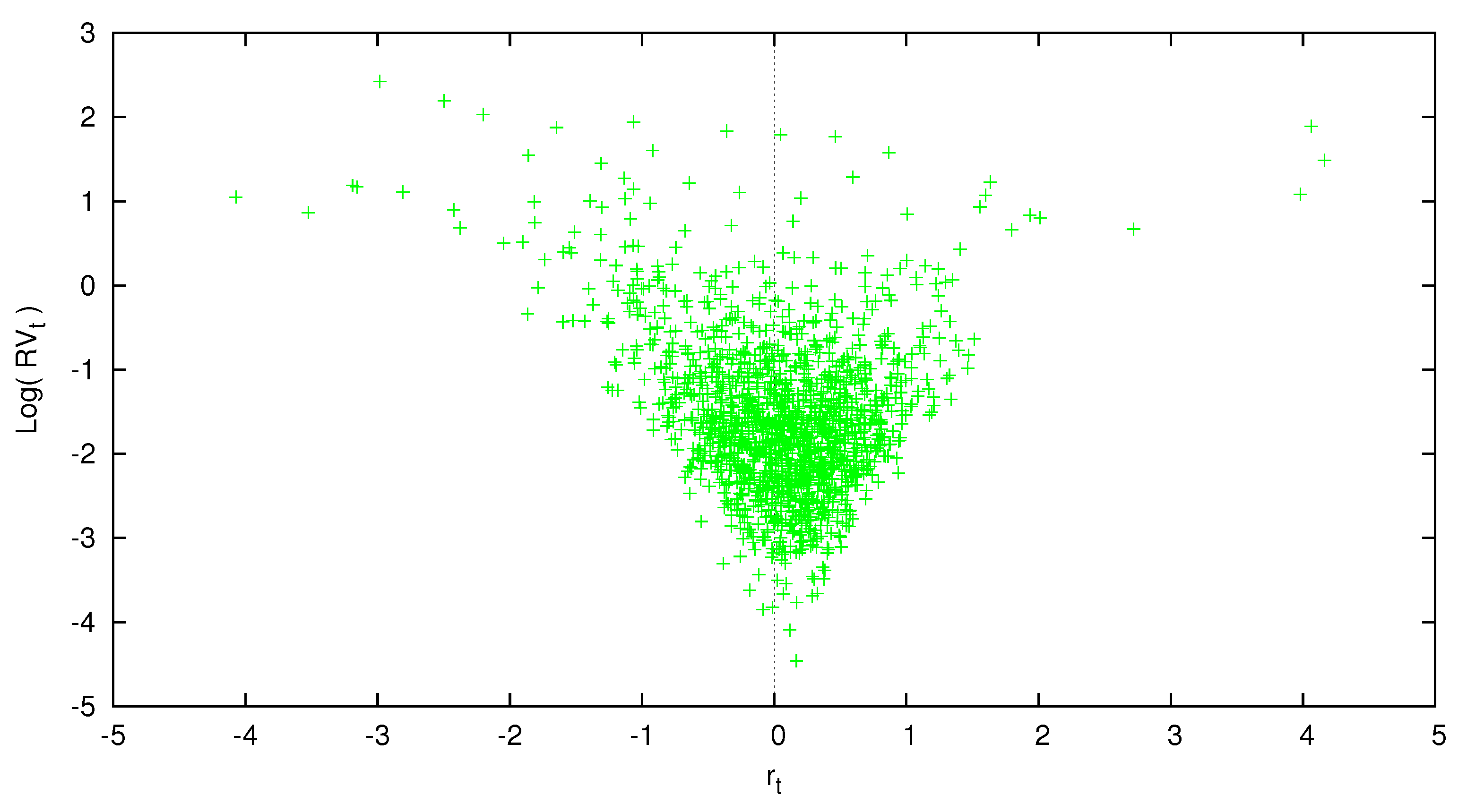
Table 1 reports various summary statistics for monthly excess returns and realized variance. Compared to squared returns, realized variance is less noisy. Returns standardized by realized variance are approximately normal with sample skewness of 0.003 and sample kurtosis of 2.6856. Log-realized variance is closer to being bell-shaped than the levels of . Figure 1 displays a scatter plot of market excess returns and which is the basis of our time-series models.
3. Risk Return and Volatility Feedback
This section will provide some motivation for the econometric model studied in this paper. Consider the following specification based on Equation (7) from French et al. (1987) for excess returns
The first term on the RHS is the expected excess return conditional on the information set . Hence, it can be a function of . In French et al. (1987), the first term comes from an ARMA model on realized variance or standard deviation. This component is ex ante and captures the traditional positive risk–return relationship that the literature has focused on.
The second term of Equation (2) is the volatility innovation and is the ex post adjustment that volatility feedback operates through. If variance risk is priced, an unexpected increase in stock market volatility raises future required stock returns, and thus lowers stock prices (see Campbell and Hentschel (1992)). In this case, would hold. Therefore, if volatility is priced, a positive shock to volatility will have a positive impact on the first term and a negative effect on the second term. Thus, volatility feedback obscures any risk–return relationship. Note that, in this specification, only when the variance shock is zero () does the conditional mean of excess returns contain a pure risk–return effect.
Our goal is to nonparametrically model these two components of excess returns. To fully capture the two opposing effects on excess returns, it is critical to jointly model excess returns and the contemporaneous variance. In addition, the conditional mean of excess returns should be a function of the ex post variance. The other conditional expectations we will model nonparametrically. These considerations lead to a nonparametric joint model of excess returns and log-realized variance.
4. Nonparametric Model of Market Excess Returns and Realized Variance
In this section, we provide the intuition behind the nonparametric model that we will use to flexibly estimate the joint relationship between excess returns and contemporaneous realized variance. As pointed out by Brandt and Kang (2004), there are no theoretical reasons that a particular parametric relationship should hold between the conditional mean and variance of excess returns. Without a theoretical relationship to guide us, we choose to let the data inform us about the risk–return trade-off by modeling the joint probability distribution of excess returns and realized variance as an unknown distribution and fitting it nonparametrically.
Our nonparametric approach consists of approximating the unknown joint distribution’s density with the infinite mixture of bivariate densities
where are the mixture probabilities such that , , and , and are the mixture parameters. The function is the jth mixture components smooth, bivariate, probability density function given the mixture parameter and information set .
It it well understood that any continuous bivariate distribution can be approximated to arbitrary accuracy by selecting an appropriate density function for and by estimating the unknown mixture weights and mixture parameters , for (Ghosal et al. 1999). In the next section, we discuss how the infinite number of unknowns can be estimated with a finite number of observation. For now, we only consider how we can obtain a nonparametric representation of the risk–return relationship from Equation (3) through the conditional distribution of excess returns given log-realized variance. To reduce the clutter from carrying around excessive notation on the conditional mixture arguments, we drop and from when it is clear to do so.
By the law of total probability, the joint distribution in Equation (3) can be written as the product of the marginal and conditional distributions
Drawing on the theoretical considerations of Andersen et al. (2003), the known empirical bell-shaped distribution of , and the approximately normally distributed standardized excess returns, we choose to let the conditional and marginal probability density functions be
where is the normal density function with mean and variance . The jth-cluster’s mixture parameter vector is and the conditioning set is . Although the jth mixture component in Equations (5) and (6) are normally distributed, mixing them over the infinite set of different valued s produces joint distributions of excess returns and log-realized variances with non-zero higher ordered moments, multiple modes, and a wide variety of curvatures.
What is novel about Equations (5) and (6) is that their mixture locations and scales are functions of contemporaneous and lagged realized variances and lagged returns. Previous infinite mixture models directly mix over the conditional means and variances and do not allow for covariates in the mixture moments. By including contemporaneous and intertemporal variables, our mixture model’s means and covariances explicitly depend on intertemporal values of returns and volatility and contemporaneous values of volatility. For example, the values of can impact the mixture means and variances of excess returns. Note that, under certain conditions, will be an unbiased estimate of the variance of returns, but we allow for deviations that are captured by the s in the mixture model.
Although not the focus of this study, the model allows for a leverage effect or asymmetric response of past return shocks to future . This occurs in Equation (6) through the terms and and, since this enters the mixture, allows for a general nonlinear leverage effect.
The intertemporal form of Equations (5) and (6) is not based on theory, but on empirical regularities known to exist in stock market returns and their volatility. For instance, the conditional mean of in Equation (6) is along the lines of the models found in Andersen et al. (2007), Corsi (2009) and the joint models of Maheu and McCurdy (2007, 2011), as adapted to monthly data. It features an expected volatility comprised of an intertemporal six month component that captures the significant persistence known to exist in realized variances.8 The last two terms of the conditional mean in Equation (5) also accounts for an asymmetric volatility relationship by including an asymmetric response in the mixture means of log-realized variances to lagged returns.
In the conditional density of Equation (5), any potentially nonlinear function of can be conditioned on; e.g., or . This conditional density function of excess returns captures the empirical regularity of excess returns being normally distributed when standardized by . The conditional mixture mean implicitly includes a risk–return relationship (positive) as well as a volatility feedback effect (positive or negative).9 As a result, the signs of the mixture parameters s are left ambiguous. Essentially, we are nonparametrically modeling through Equation (3), Campbell and Hentschel (1992) reduced form equation of excess returns without imposing any theoretical restrictions. For this reason, we place no restrictions on the and , . The implications for the risk–return trade-off can be indirectly derived from the contemporaneous model and are discussed later.
4.1. Conditional Distribution of Returns Given Realized Variance
From the mixture representation of the joint distribution of excess returns and realized variances in Equation (3), it directly holds that the probability density function of excess returns conditional on contemporaneous log-realized variance equals
where is the conditional probability density function of the jth cluster and is the associated marginal density function for .
The mixture weights in Equation (8) have the particular form
so that they sum to one. From Equation (10), we see that those clusters providing a better fit of receive more weight in the mixture representation. Components whose and result in larger likelihoods play a bigger role in accounting for the risk–return trade-off and the volatility feedback effect. Note that different values of produce smooth changes in the conditional distribution of excess returns and, hence, in its mean.
Our interest rests in the risk–return and volatility feedback relationship; in other words, the conditional expectation of market excess returns given log-realized volatility. Since the expectation of a mixture distribution is equivalent to the mixture of the expectations, from the conditional mixture means of excess returns in Equation (5), the expectation of Equation (8) is the conditional expectation
A linear parametric risk–return relationship is nested in Equation (11) by simply letting there be only one mixture component. As more mixture components are added and a greater mixture of differently valued s and s are included, the conditional mean of excess returns as a function of , moves away from linearity. This mixing allows Equation (11) to become more flexible and capable of modeling a wider array of different types of risk–return and volatility feedback relationships.
Being a function of realized variance, the mixture representation in Equation (11) differs from previous work by nonparametrically modelling excess returns and ex post variance. The conditional mean of excess returns given realized variance will contain an ex ante risk–return component and an ex post volatility feedback component.
A plot of the conditional expectation of excess returns as a function of will be a smoothly changing function that weights each of the cluster specific conditional expectations according to how the weight function changes as changes. This is true even if each cluster’s expectation, , is constant. In this way, we can see the contemporaneous relationship of log-volatility on the conditional mean of excess returns. As mentioned above, volatility feedback occurs simultaneously and this specification is designed to shed light on it.
4.2. Dirichlet Process Prior for the Infinite Number Of Unknowns
Because our nonparametric model of excess returns and log-realized variance joint probability distribution consists of an infinite number of unknown mixture weights, , and parameter vectors, , we resort to a Bayesian prior to shrink the number of unknowns to a feasible number while not forsaking the flexibility that comes from an infinite mixture model. The prior we choose is the Dirichlet process prior (DP). The Dirichlet process prior has a long history, beginning with Ferguson (1973), of use in Bayesian nonparametric problems. It was used as a prior in countable infinite mixtures for density estimation in Ferguson (1983) and Lo (1984), but applications were limited until modern computational techniques. The seminal paper by Escobar and West (1995) shows how to perform Bayesian nonparametric density estimation with Gibbs sampling.
The DP prior essentially partitions the parameter space into a finite number of sets such that parameter vectors drawn from a particular set all have the same unique value. Such a prior promotes clustering among the mixture components resulting in only having to estimate a few unknown mixture parameter vectors. The probability of a particular mixture parameter vector occurring is equal to the probability over a member set of the partition as defined by the DP prior.
To be explicit, we assume the Dirichlet process prior, , for the unknown and , of Equation (3). Sethuraman (1994) shows that a prior for the mixture unknowns has the representation of being almost surely draws from
for . In Equation (13), each mixture cluster parameter vector is a unique vector independently drawn from the base distribution . This base distribution is our best guess at how the s are distributed. In Equation (12), the mixture weights are drawn from what is referred to as a stick breaking process since the unit interval is successively broken into the mixture weights, , , by breaking off random portions of the remaining part of the unit length stick. This stick breaking process ensures the mixture weights sum to one while also promoting clustering in the s.
The positive scalar , known as the Dirichlet processes’ concentration parameter, controls the degree of clustering in the mixture components. A close to zero results in only a few mixture weights being nonzero, putting most of the weight on only a few unique draws from . As gets larger more s become nonzero, and, hence, there is less clustering and more unique s. In the limit as approaches infinity, the partition of the mixture parameter space is no longer finite and discrete. Instead, the parameter sets within the partition becomes so fine and large in number that the s no longer cluster to a finite set of unique value but instead will be continuously distributed as . In other words, when , the mixture weights are uniformly distributed, no clustering occurs and the prior for the s is essentially .
4.3. Hierarchical Representation
The Dirichlet process mixture model defined in Equations (3)–(6), (12) and (13) also has the hierarchical representation where is distributed
In Equation (15), the distribution of the parameter vector is the unknown distribution, G, whose prior is modeled in Equation (16) by the Dirichlet process prior . Given the stick breaking definition of the Dirichlet process in Equations (12) and (13), the prior distribution for G is almost surely equal to the discrete distribution
where denotes a point mass at , and and are the random realizations defined in Equations (12) and (13).
Equation (17) helps us better appreciate the clustering behavior of the DP prior. Since G is almost surely a discrete distribution, there will be duplicates among the , . As a result, several of the observations will share the same mixture parameter vector, .
If volatility risk is priced, a positive volatility shock requires an increase in returns which discounts all future cash flows at a higher rate. This discounting results in a drop in the current price. As a result, if any unexpected news arrives be it good or bad, uncertainty increases causing the innovation to volatility, , to be positive. If a volatility feedback effect exists the effect good news has on returns will be dampened, whereas the effect of the bad news will be amplified. Therefore, a price increase from good news will be less than what would occur without volatility feedback while a price decrease from bad news will be steeper. Dynamics of this sort occur when is negative. On the other hand, if volatility shocks are small, the net impact on the conditional mean of excess returns will be a reward for risk which can be captured by a positive .
By connecting the clustering property of the DP with the volatility feedback parameter, , our nonparametric model will have a unique during similar market environments. Two months with similar market behavior will have the same volatility feedback, . However, the volatility feedback for months where the market dynamics are different will not equal .
4.4. Posterior Simulation
To sample the posterior density of our nonparametric joint distribution model, we will exploit the mixture representation in Equation (3) and a slice sampler based on Walker (2007); Kalli et al. (2011); and Papaspiliopoulos (2008).10 This Markov chain Monte Carlo (MCMC) algorithm introduces a random auxiliary, latent, variable, , which slices away any mixtures clusters with a weight less than . In this way, the infinite mixture model is reduced to a finite mixture.
Introducing the latent variable , we define the joint conditional density of the observed variables and as,
This infinite mixture is truncated to only include alive clusters with while dead clusters have a weight of 0 and can be ignored. If has a uniform distribution, then integration of with respect to gives back the original model . On the other hand, the marginal density of is .
We augment the parameter space to include estimation of . Let , and , then the full likelihood is
and the joint posterior is
where the number of mixture clusters, K, is the smallest natural number that satisfies the condition . This value of K ensures that there are no for . In other words, we have the set of all clusters that are alive, .
Posterior simulation consists of sampling from the following densities:
- , , .
- , , with
- , .
- Find the smallest K such that .
- , RV.
where and .
The first step depends on the model and the base density to the DP priors’ base measure, . For the kernel densities in Equations (5) and (6), specifying a normal prior for the regression coefficients and an independent inverse gamma prior for the variance, in other words, defining , we can employ standard Gibbs sampling techniques in Step 1 (see Greenberg (2013) for details on the exact form of these conditional distributions). Step 2 results from the conjugacy of the generalized Dirichlet distribution and multinomial sampling Ishwaran and James (2001). Given and S, each is uniformly distributed on . The next step updates the truncation parameter K. If K is incremented, Step 4 will also involve drawing additional and from the DP prior. The final step is a multinomial draw of the cluster assignment variable based on a mixture with equal weights.
Repeating all these steps forms one iteration of the sampler. The MCMC sampler yields the following set of variables at each iteration i,
Note that , implies , through Equation (12). After dropping the burn-in phase from the above sampler, we collect samples.
Each ith iteration of the algorithm produces a draw of the unknown mixing distribution G from its posterior as
We will make use of these posterior realizations of G to form the predictive density and conditional expectations.
5. Nonparametric Conditional Density Estimation
To flexibly estimate the conditional density found in Equation (8), or the conditional mean in Equation (11), we use the method of Muller et al. (1996). This is an elegant approach to nonparametric estimation that allows the conditional density and expectation of excess returns to depend on covariates, in this case . The method requires the joint modeling of the predictor variable and its covariates and uses well know estimation methods for Dirichlet process mixture models. We extend Muller et al. (1996) to the slice sampler to accommodate the non-Gaussian data densities and nonconjugate priors found in our nonparametric model of market excess returns and realized variances.11
Based on the previous section, and given , the ith realization from the posterior of the joint conditional predictive density for the generic return, log-realized variance combination, , is
where the predictive is conditional on the information set .
Substituting in the stick breaking representation for found in Equation (22), the posterior draw of the predictive density has the equivalent representation
where is the expectation of Equation (14) over . To integrate out the uncertainty associated with G, one averages Equation (24) over the posterior realizations, , , to obtain the posterior predictive density
Now, the predictive density of r given can be estimated as well. For each draw of , we have
where is the conditional density of Equation (5), is the marginal density of Equation (6) and
The denominator of is the marginal of Equation (24) obtained by integrating out r. is the marginal data density of for the jth cluster with the marginal cluster parameter and is the marginal data density with mixing over the base measure. The terms in Equations (26) and (27) involving are defined as follows:
Assuming that the marginal data density is available in analytic form, both of these expressions can be approximated by the usual MCMC methods. For instance, , where , with a similar expression for the numerator of Equation (28).
The posterior predictive conditional density is estimated by averaging Equation (26) over the posterior simulations of as
Using this approximation, features of the conditional distribution such as conditional quantiles can be derived.
Nonparametric Conditional Mean Estimation
Our focus will be on the conditional expectation that can be estimated from these results. First, the conditional expectation of r given , and the information set is
where is taken with respect to Equation (28). Note that this final term is only a function of and can be computed once, at the start of estimation, for a grid of values of . It is estimated as12
for , .
Given , Equation (31) shows the conditional expectation of r is a convex combination of cluster specific conditional expectations , , along with the expectation taken with respect to the base measure . The weighting function changes with the conditioning variable , which in turn changes for each .
Finally, with this, we can obtain the posterior predictive conditional mean estimate by averaging over Equation (31) as follows:
in order to integrate out uncertainty concerning G.13 Point-wise density intervals of the conditional mean can be estimated from the quantiles of .
We evaluate the predictive conditional mean for a grid of values over . This will produce a smooth curve and we will have a unique curve for each information set in our sample .
6. Empirical Findings
For our empirical analysis, we specify the following priors. The base measure contains priors for each regression parameter in Equations (5) and (6) as independent while and , , where denotes a gamma distribution with mean . Note that we expect the s to be close to 1 and the prior reflects this with but allows for deviations from this. These prior beliefs cover a wide range of empirically realistic values and robustness to other choices is discussed below. The concentration parameter of the Dirichlet process, , is estimated and has a prior . Each cluster contains the nine parameters found in .
We use 5000 initial iterations of the posterior sampler for burn-in and then collect the following 20,000 for posterior inference. The Markov chain mixes well and the posterior mean (0.95 density interval) for is , and the posterior mean (0.95 density interval) for the number of alive clusters is , . In other words, about 2.6 components are used to fit the joint model of and .
Before we turn to the estimates from our nonparametric DPM model, a parametric version of the model is reported in Table 2. This is a one state model. The coefficient on in the excess return equation is significantly negative and hence evidence of the volatility feedback mechanism at work. is close to 1 and indicates no systematic bias in . The estimates of and indicate persistence in . The lagged standardized excess return terms entering the log-volatility equation show asymmetry. A negative return shock results in a larger conditional mean for log-volatility next period compared to a positive shock.
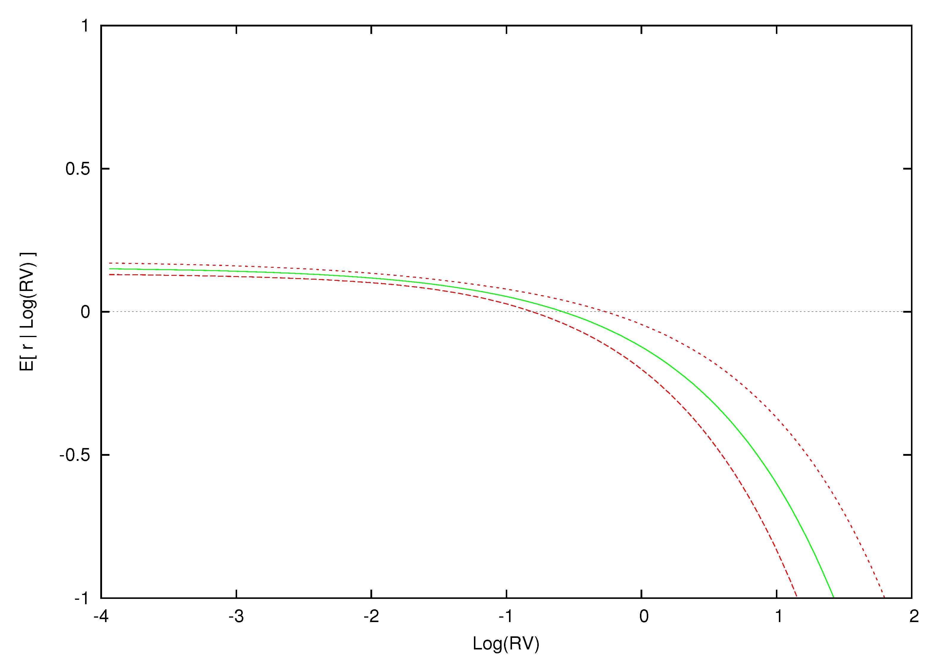
Figure 2 displays the contemporaneous relationship between expected excess returns and for the estimated parametric model.14 The conditional expectation of excess returns given log-realized variance is computed over a grid of 100 log-variance values between to 2.0. Using a straight line, we interpolate between the values of at the different values of log variance in order to approximate the smooth relationship between and . Although the estimated model is a fixed linear relationship between excess returns and , this parametric model yields the nonlinear relations between the conditional mean of excess returns and log-realized variance found in Figure 2.
In Figure 3, the conditional expectation of excess returns as a function of log-realized variance for our nonparametric model is plotted for every information set, , , in our dataset. Note that the parametric relationship in Figure 2 is the same for every information set and is not affected by low or high volatility periods. Overall, there is a general increase in the conditional mean of excess returns in Figure 3 as log-realized variance increases from low levels of volatility to a point where expected returns become negative. This is a general pattern found in all of the plots of Figure 3. However, the log-variance argument that causes the conditional mean of excess returns to begin to decline does differ for the different information sets . It is clear that, if one averaged over these expectations, you could obtain a positive value for expected excess returns or a negative value.15 To really understand the relationship between the conditional mean of excess returns and log-realized variance, we need to consider the conditional expectation and the innovation of log-volatility as well.
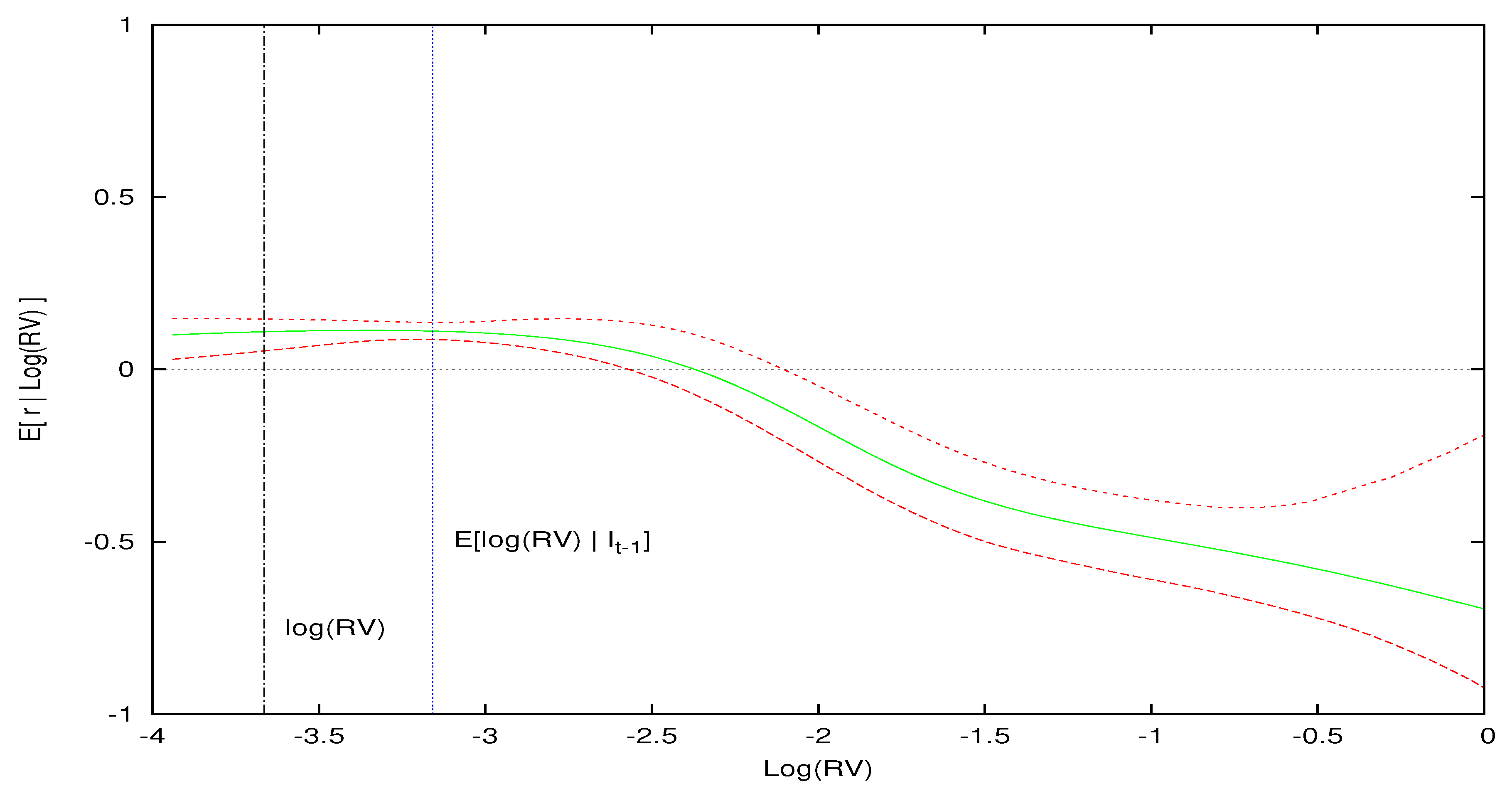
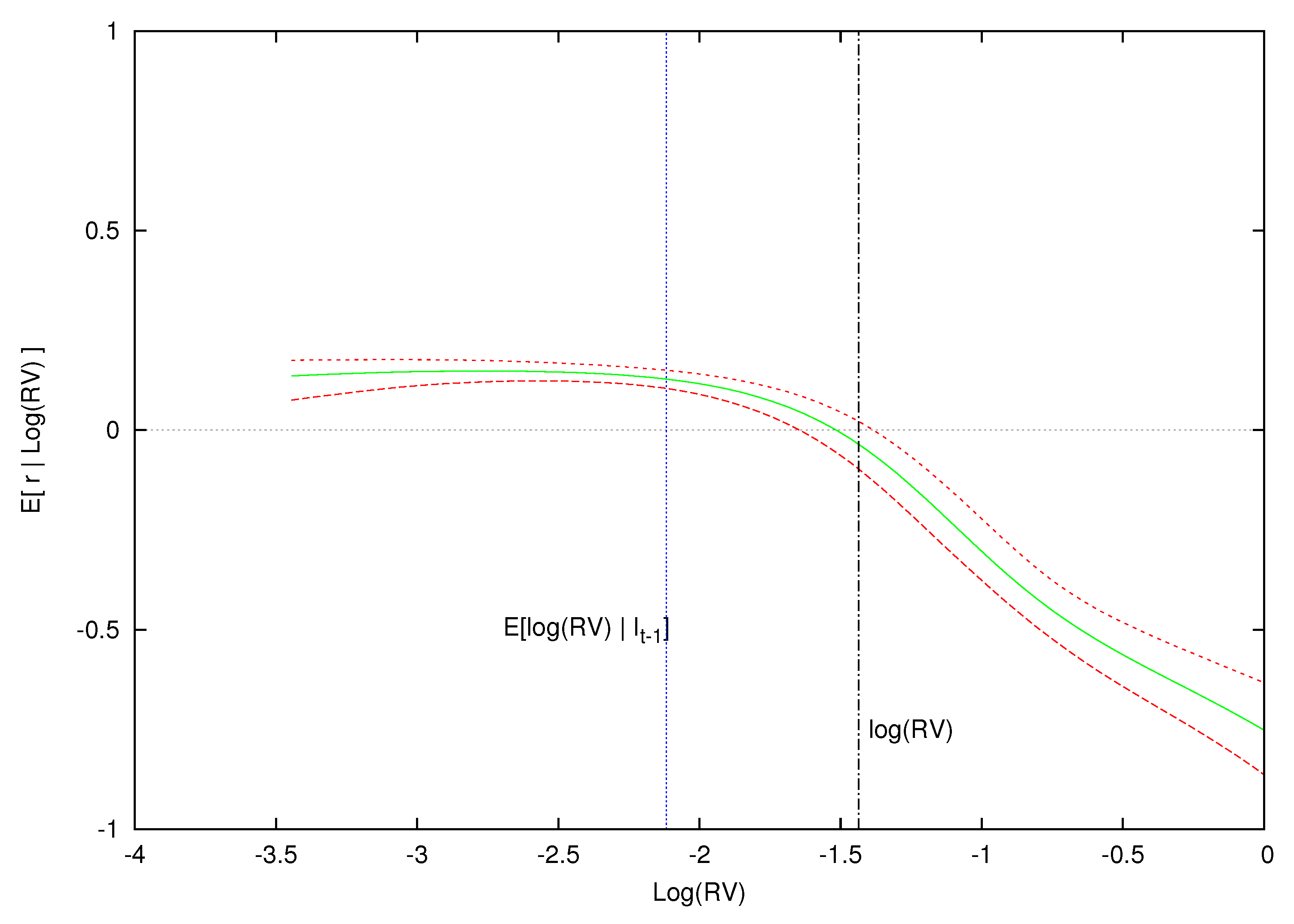
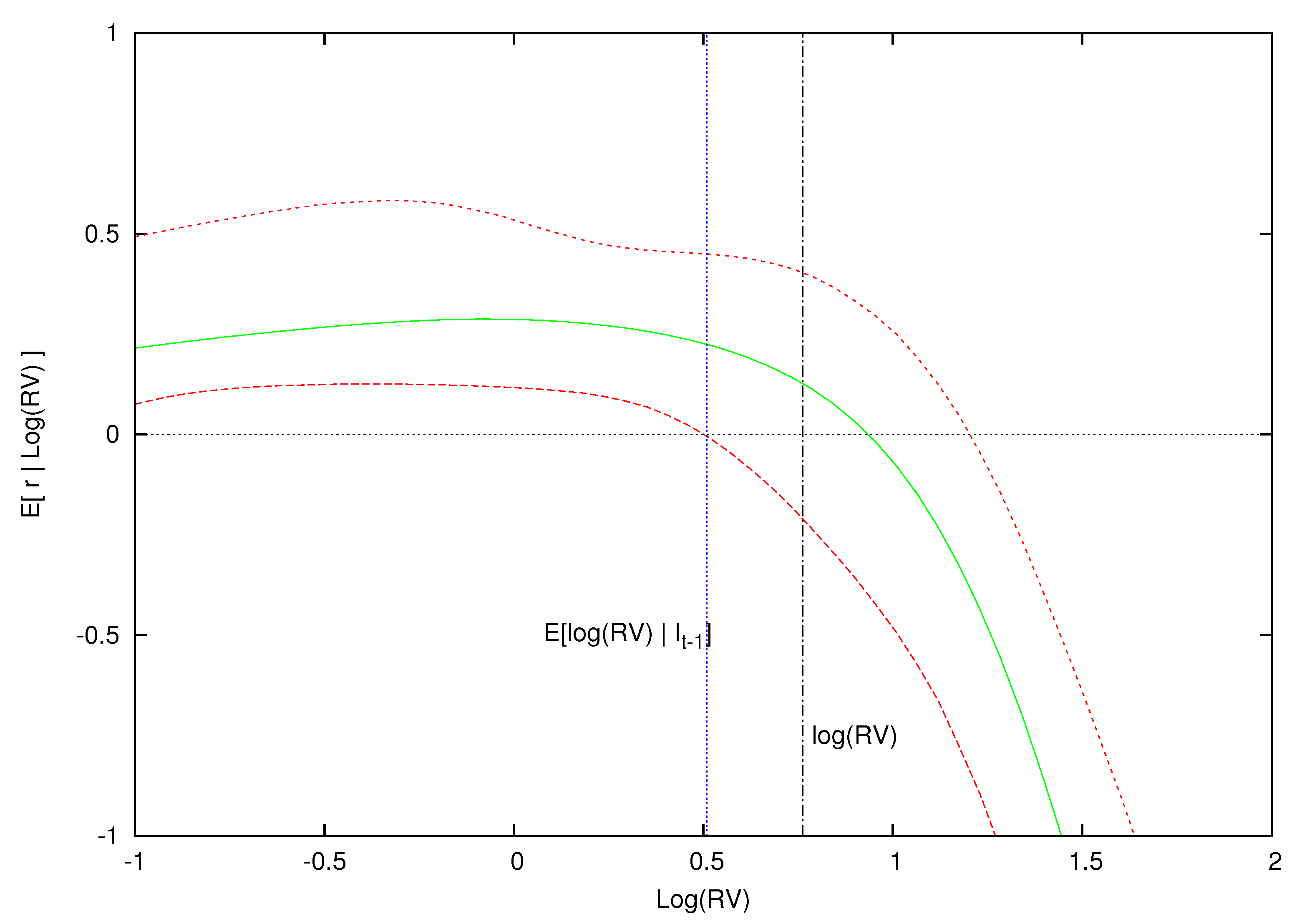
To do this, we isolate three months in our sample where market volatility is low (October, 1964), average (February, 1996) and high (December, 2008) and plot in Figure 4, Figure 5 and Figure 6 the conditional expectations of excess returns against different values of log-realized variance during these three months. In addition to plotting the conditional expectation of market excess returns, the three figures also include the conditional expectation of log-realized variance, , as a vertical blue line, and the observed realized value of log-realized variance for that month, , as a vertical dashed line. Point-wise 90% probability density intervals are included for the expected excess return.
6.1. Volatility Effect
Recalling our discussion on volatility feedback, if volatility is priced and a positive volatility shock arrives, then, all things being equal, the required rate of return increases which discounts all future cash flows at a higher rate and results in a simultaneous drop in the current price so as to deliver a higher future return consistent with the increase in risk. Only when the observed log-variance is equal to its expected value will the volatility feedback effect be zero. Hence, if volatility risk is priced, values of log-variance greater (less) than its expected value will cause current prices to fall (rise).
This is exactly what we find in Figure 4, Figure 5 and Figure 6 for an unexpected positive volatility shock where log-variance is greater than the expected value of log-realized variance. For instance, consider Figure 4, which conditions on the low volatility information set, .16 In this month of low market volatility, the model’s expected log-realized variance is . The expected excess return is positive for values of log-variance below and slightly above this expected value, but eventually the expected excess return becomes negative as increases above . In other words, when market volatility is low, if the volatility shock is sufficiently larger than zero, we expect a contemporaneous decrease in prices from the volatility feedback effect.
Figure 5 displays a similar pattern for the month where volatility is not unusual but typical for the equity market. The period is for the information set and our model finds the expected value of to be . As before, expected excess returns are positive for values of log-variance less than and slightly greater than , but eventually becomes negative when log-realized variance is larger than . If the log-volatility shock is sufficiently large (about +0.68), then the expected excess return is negative and continues to decrease as the size of the volatility shock grows. In addition, notice that the whole posterior curve of has shifted rightward as the expected has increased from Figure 4 to Figure 5 (low to average ). This suggests an increase in compensation for the higher perceived volatility risk when the market moves from an unusually calm market to one that is typical.
A highly volatility market corresponding to the information set is found in Figure 6. Just as before, is essentially linear and flat for values of smaller than . In other words, the expected excess returns do not respond to negative volatility shocks. However, for values of greater than , expected excess returns start to decline and become negative when log-realized variance is almost one.17 This is consistent with the volatility feedback effect. Note that, in each of these three figures, the effect of volatility feedback on returns gets stronger where the impact of a positive volatility shock on expected returns increases as the the market moves from a low volatility state to a market with average volatility and then to a market where volatility is exceptionally high.
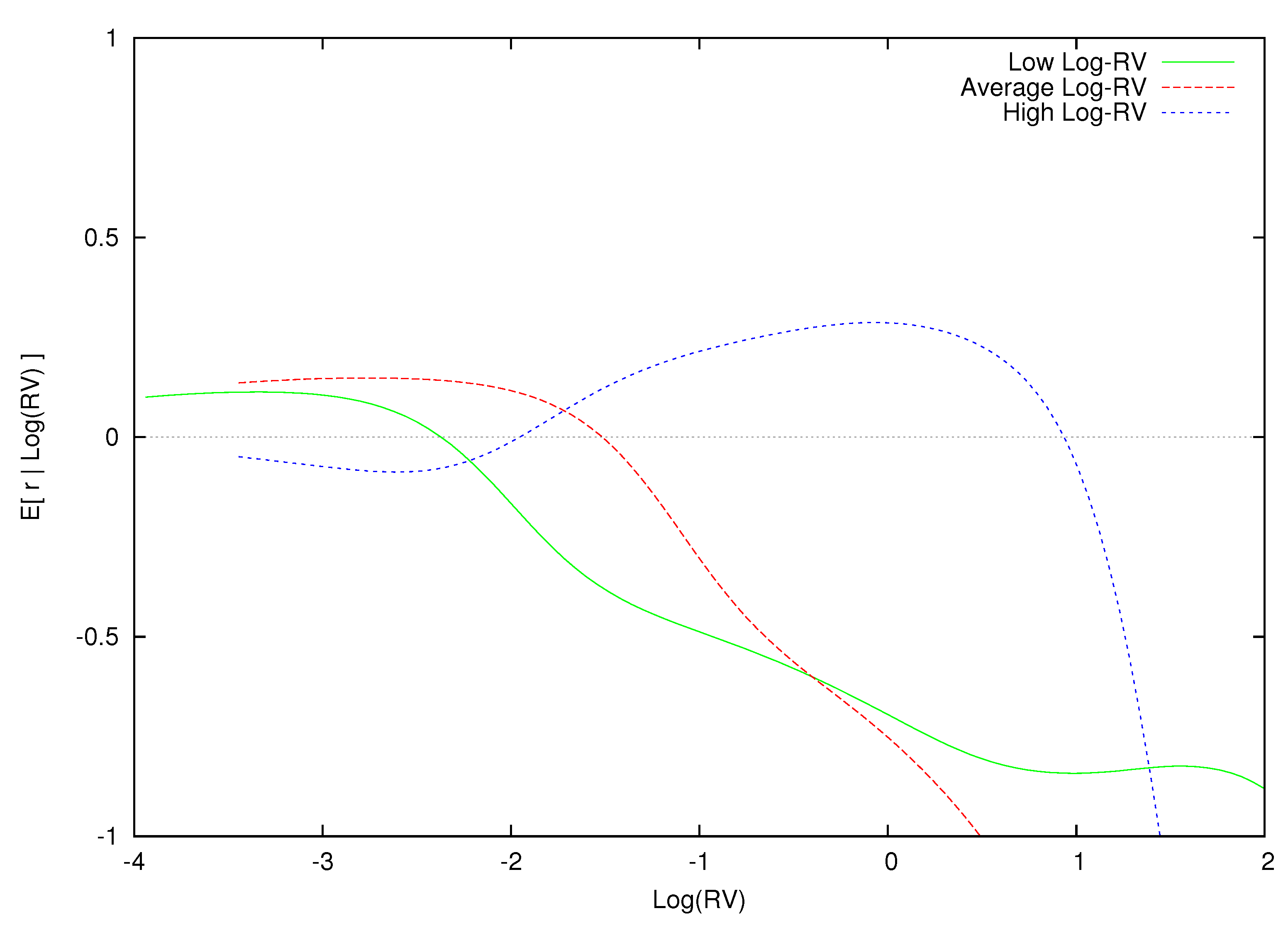
Figure 7 plots for each of the three information sets, and . As increases, the conditional expectation of excess returns shifts rightward and up. This is consistent with a positive and increasing reward for bearing higher levels of risk.
In summary, we find a robust volatility feedback effect that is most notable for positive shocks to volatility. Expected excess returns are positive below but after this value eventually become negative. Thus, small news events have little effect on expected returns, whereas large news events cause expected excess returns to decline. This suggests that risk is priced and the previous figure is consistent with this.
6.2. Risk and Return Trade-Off
To focus on risk and return, we need to account for the volatility feedback effect. In each of our figures, the point on the line that corresponds to is exactly the point with no volatility feedback. This point is where the investor receives exactly the reward for risk with no adjustment for volatility feedback because the volatility shock is zero. This will be at a different place in each of our curves of . Using interpolation between each of the grid values, we can estimate the value of at for each time period t. This represents a pure risk and return relationship which nets out volatility feedback.
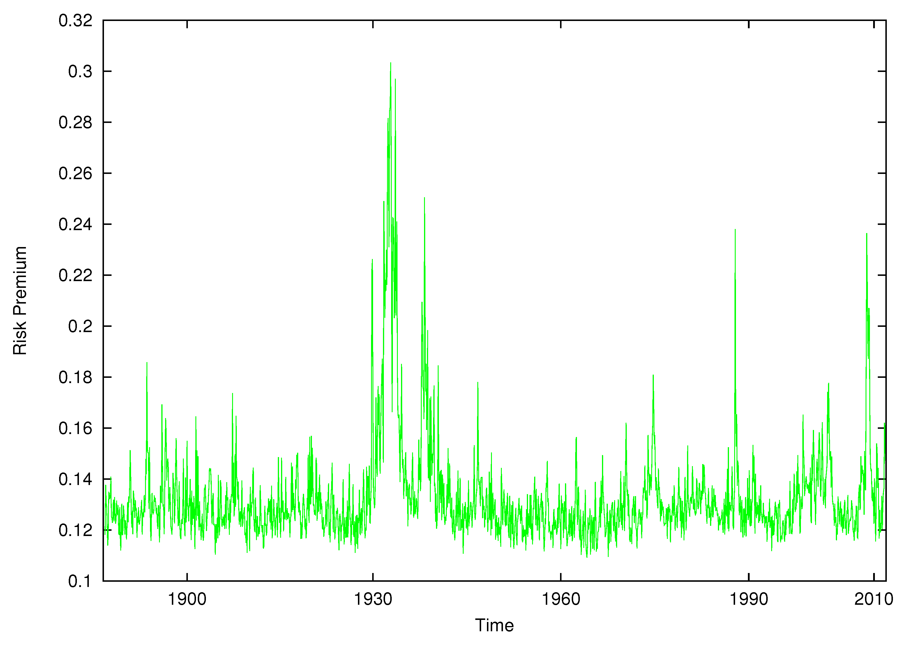
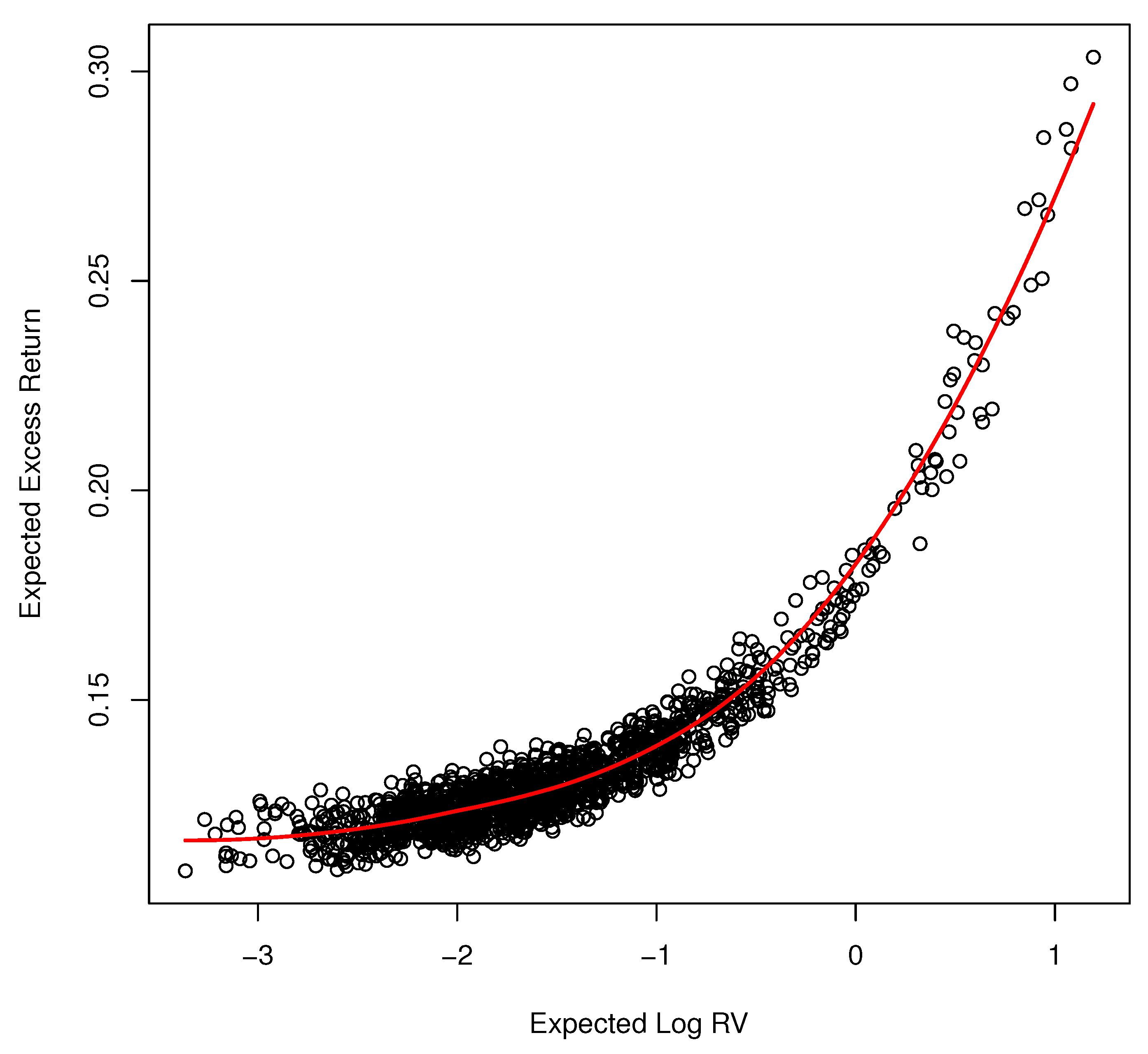
Figure 8 displays the equity risk premium over time from the nonparametric model when volatility feedback has been removed. The premium is everywhere positive. Figure 9 displays the pure risk and return relationship. It shows the expected excess return as a function of expected log-realized variance according to our model estimates when volatility feedback is removed. Each dot represents the point of in which volatility feedback is zero given the information set . The relationship is unambiguously positive and increasing in which accords with theory. The relationship is nonlinear. It is approximately linear for a small value of log-volatility but increases sharply as expected log-volatility surpasses zero.
In contrast to Campbell and Hentschel (1992) and the subsequent literature on volatility feedback, we find evidence of a positive risk and return relationship and a volatility feedback effect without imposing any economic restrictions. The key is flexibly modeling the contemporaneous distribution of market excess returns and log-realized variance and accounting for the volatility shock.
6.3. Conditional Quantiles and Contour Plots
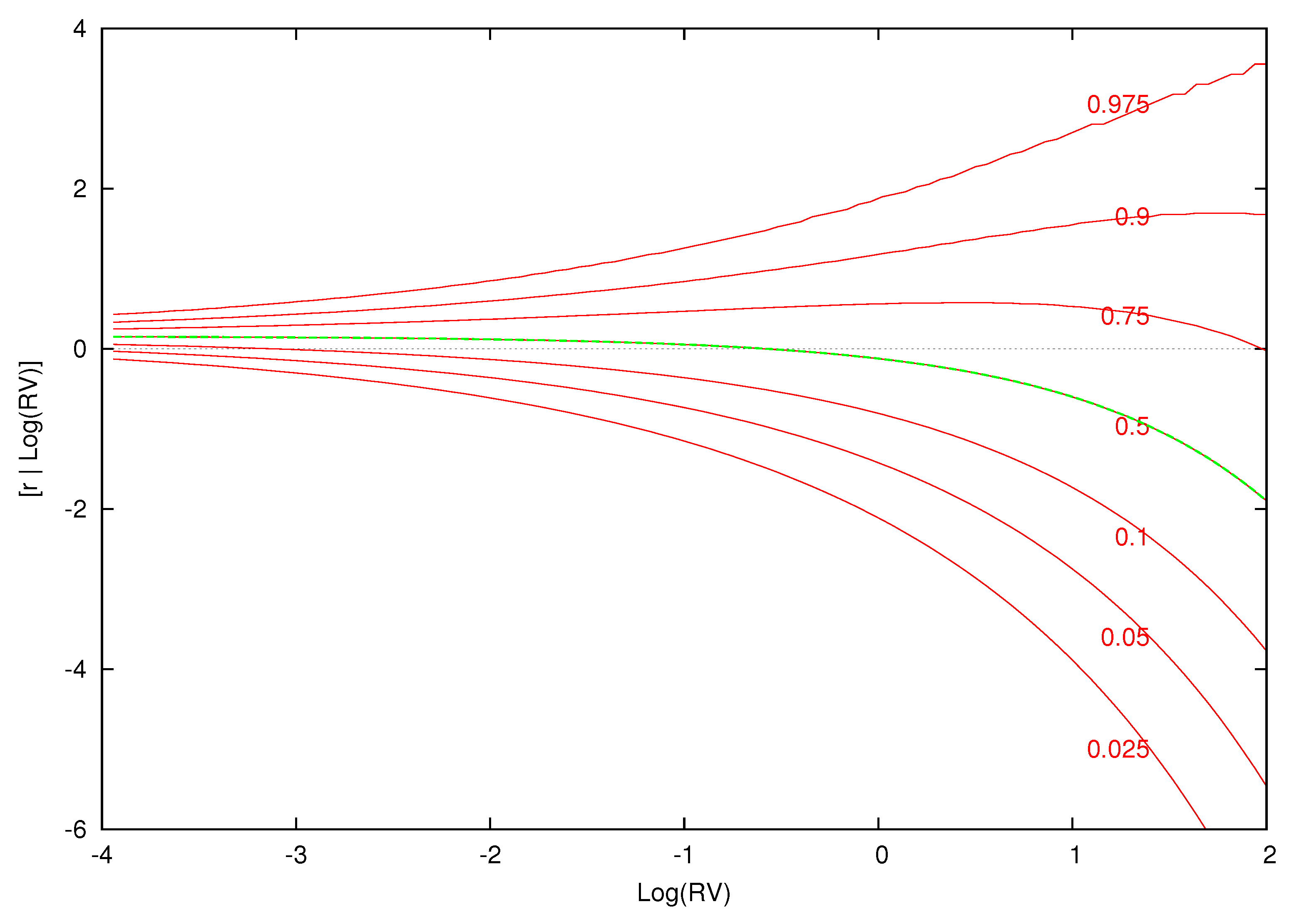
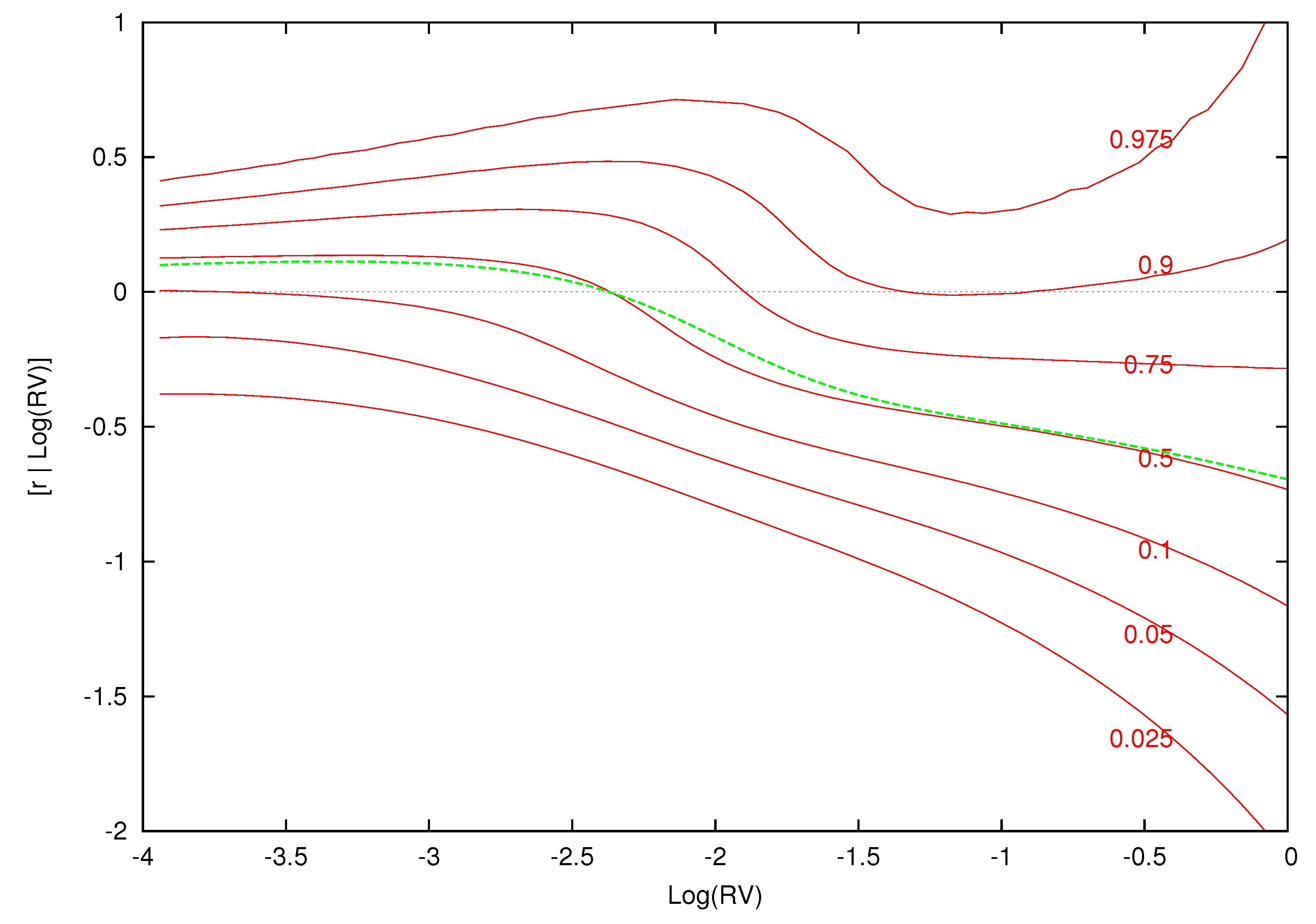
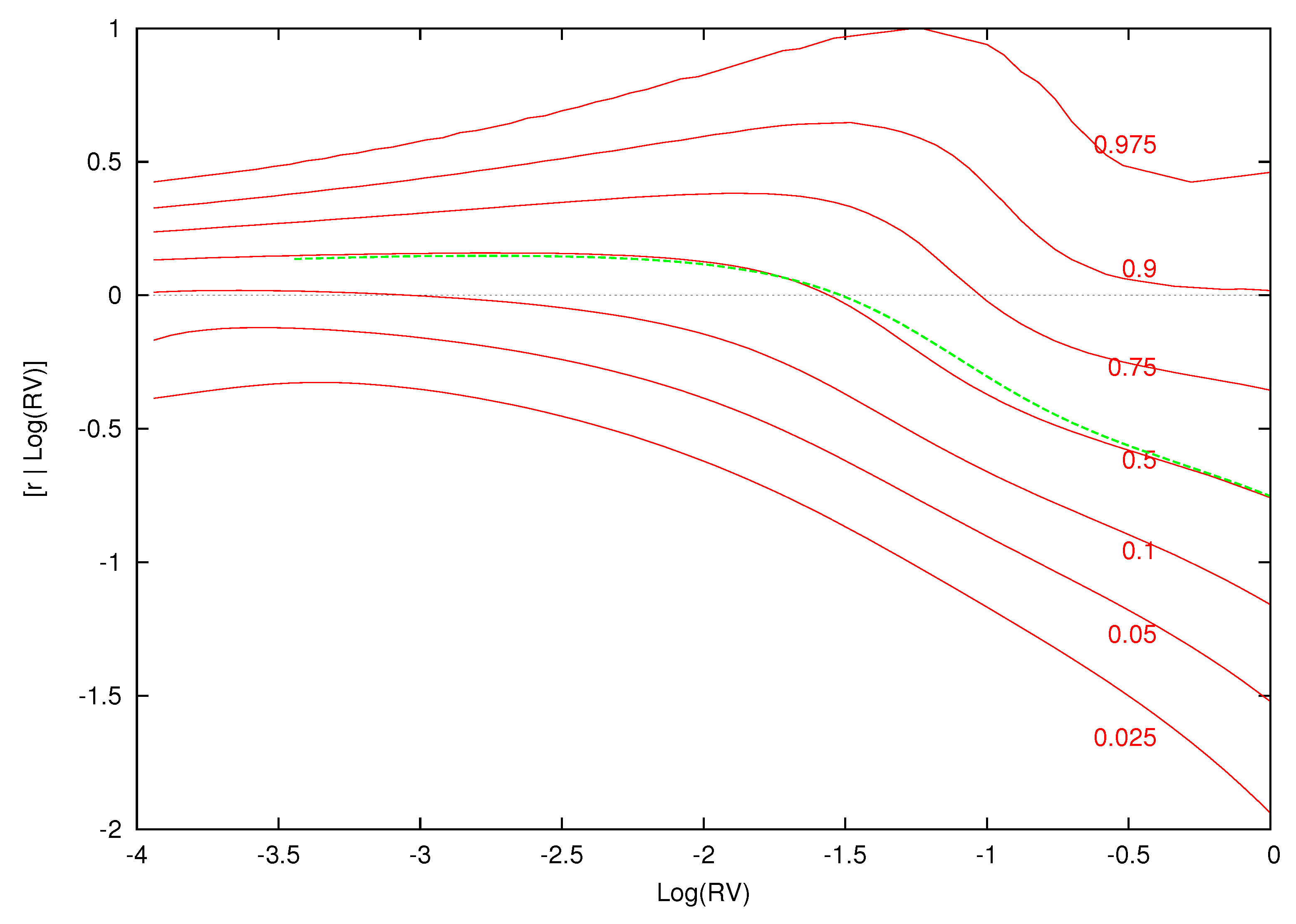
Figure 10, Figure 11, Figure 12 and Figure 13 display conditional quantile plots of the distribution of excess returns given different values of for the parametric model and several cases of the nonparametric model. In each figure, the green line is the conditional mean that was discussed above.
For the parametric model, as before, the conditional quantiles do not change for different information sets. The estimated weights and component densities in the mixture model of Equation (8), however, are sensitive to the information set and result in very different conditional distributions. Each of the conditional quantile plots show a highly nonlinear distribution that is at odds with the parametric model.
Recall from the previous discussion that the conditional expectations of the low, average and high levels of were , and , respectively. In Figure 11, Figure 12 and Figure 13, the bulk of the distribution is above zero at each of these points. Investors are most likely to receive a positive excess return from the market at the value of the expected value of log-realized variance. As increases and the volatility shock becomes larger, most of the mass in each conditional density is over a negative range of excess returns. Here, investors are likely to have a loss from investing in the market.
The upper quantiles show the most nonlinear behavior given low (Figure 11) and average (Figure 12) levels of volatility. Volatility feedback has an impact on the whole distribution and not just the conditional mean. The changes in the density, as increases, are non-monotonic. In Figure 11 and Figure 12, there is an increase in the spread of the density followed by a decrease and final increase. The point of these changes in the conditional density is to the right of the conditional mean of . The parametric quantile plot is inconsistent with these features.
Although volatility feedback is the most likely explanation of our results, Veronesi (1999) shows that, in the presence of uncertainty about the economic regime, prices overreact to bad news in good times and underreact to good news in bad times. This results in negative returns coupled with high volatility such as seen in the conditional quantile plots.
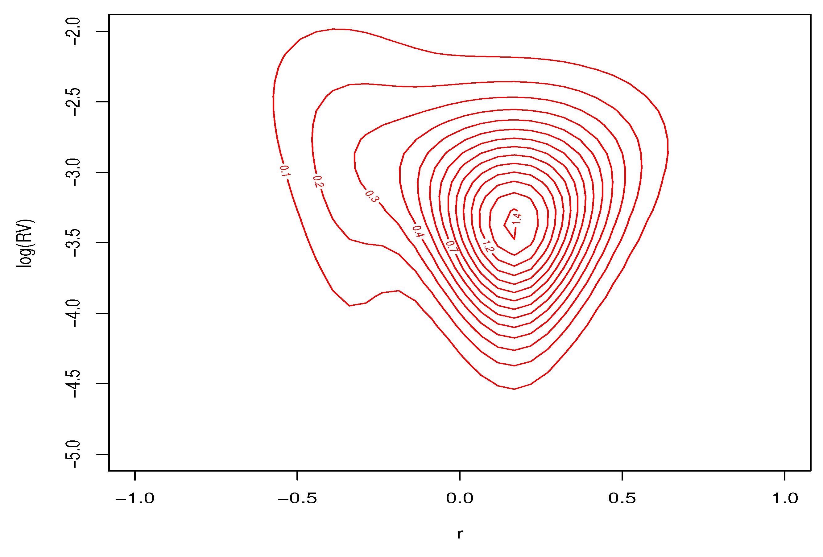
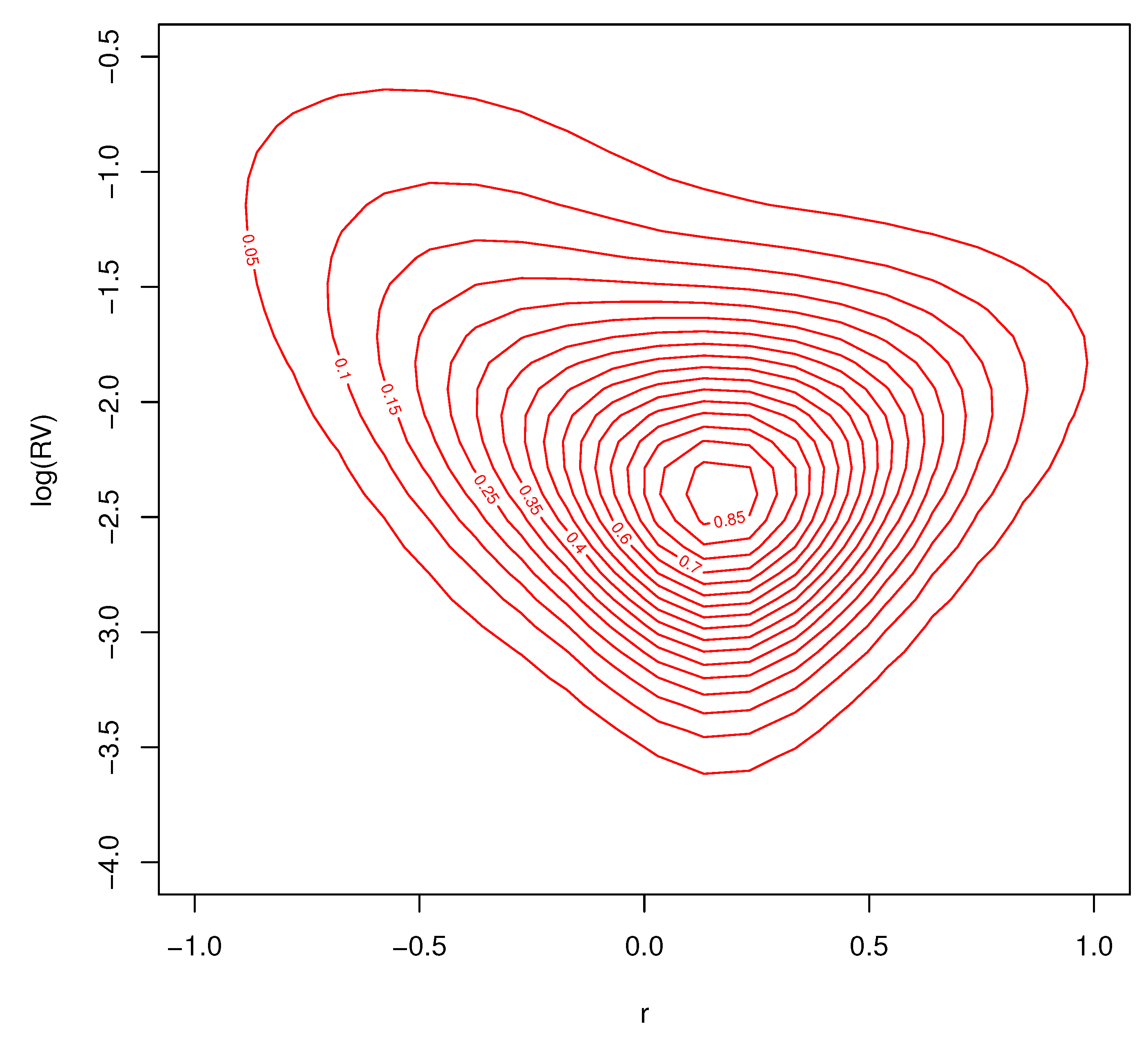
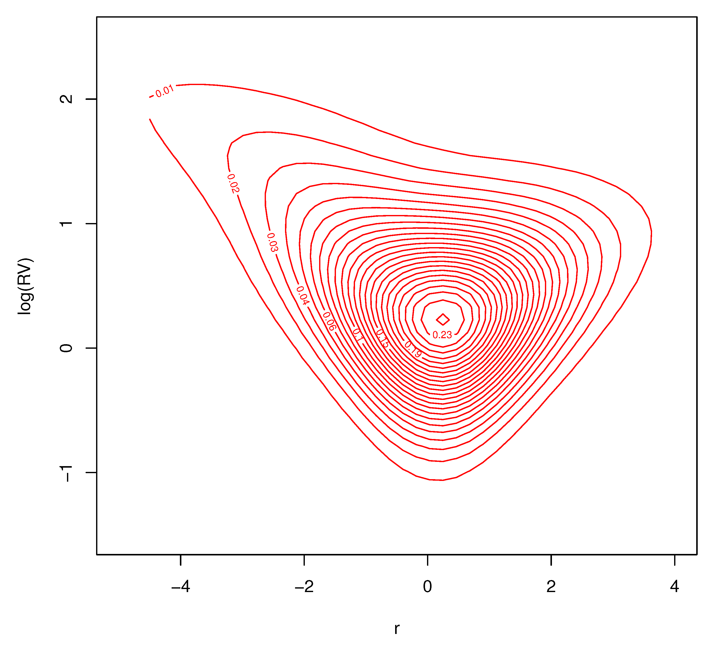
Contour plots of the conditional joint predictive density for excess returns and log-realized variances, for the three different months of market volatility, are found in Figure 14, Figure 15 and Figure 16. Each of the figures are consistent with deviations from Gaussian behavior in the conditional bivariate distribution. It is clear that the conditional distribution changes a great deal over time and is not a result of changes in location and/or scale. There is a thick tail for small values of r and larger values of in each figure, but the shape of the distributions tail is very different depending on . These important changes in the conditional density are the features that our nonparametric model are designed to capture. Conventional parametric approaches cannot accommodate these features.
6.4. Parameter Estimates and Robustness
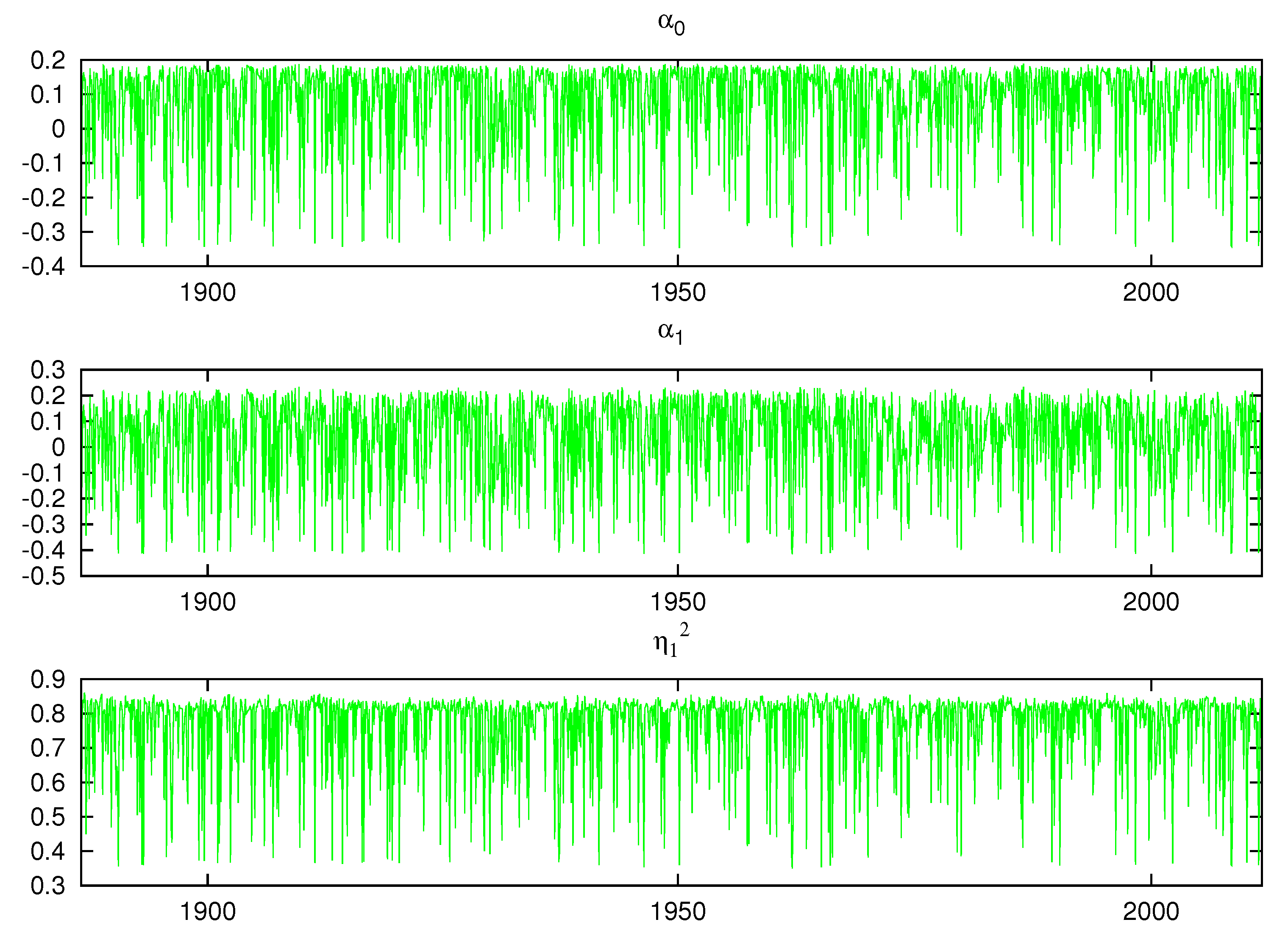
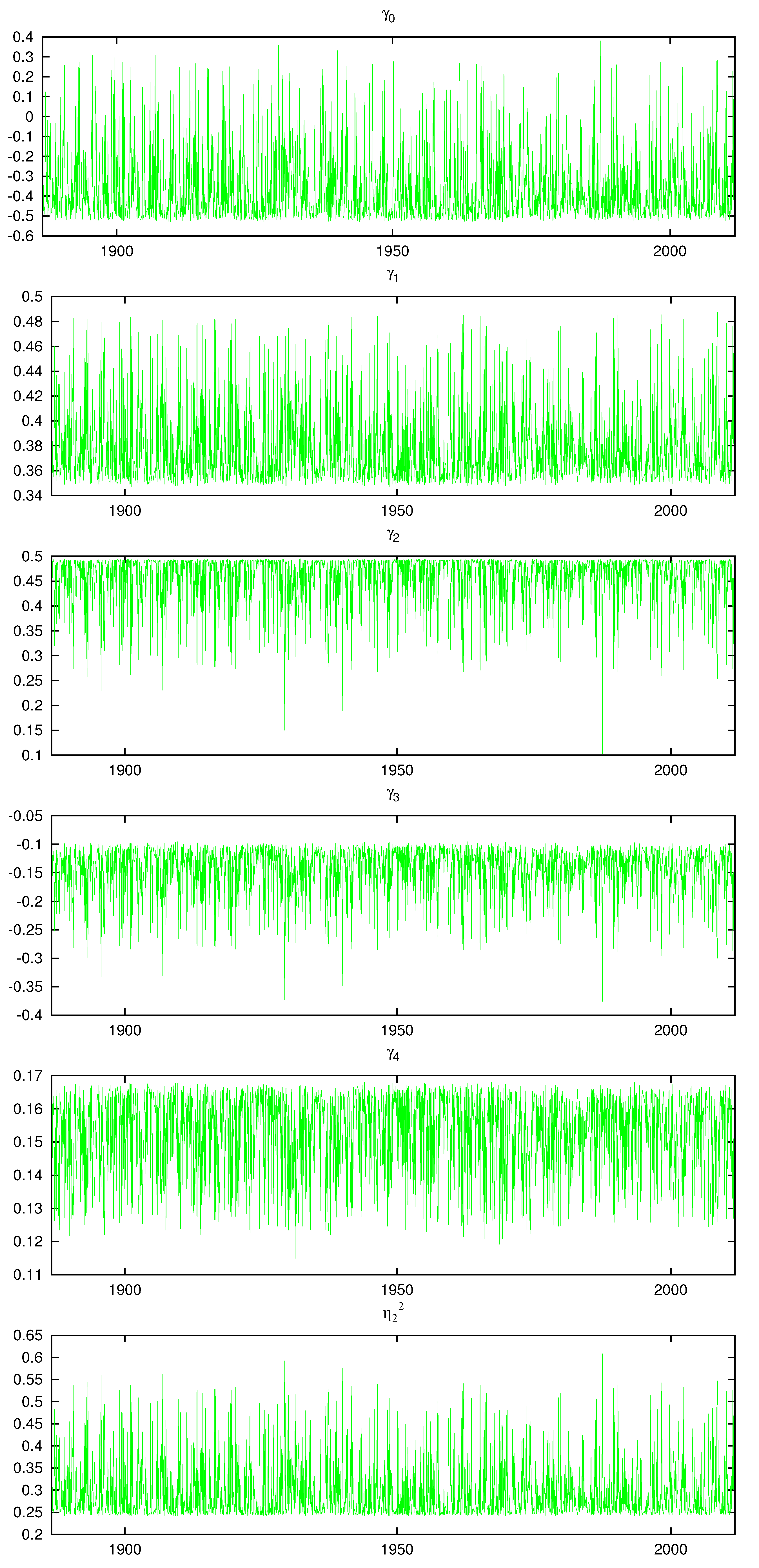
Figure 17 and Figure 18 display the posterior mean of each of the model parameters contained in the vector for . A parametric model would be a straight line. We see considerable switching between clusters in all the plots and the size of the change between the cluster’s parameter values is often large. This shows that multiple mixture components in our nonparametric model is a significant feature of the data. Compared to the parametric model results found in Table 2, , the coefficient on is negative and positive over different time periods. The variability of the parameters in the figures is well beyond the 95% density intervals for the parametric model reported in Table 2. Although the parametric model estimate of is close to one, the nonparametric parameter estimates, , , varies between 0.4 to 0.85. This is due to the significantly improved fit that the nonparametric model offers in the conditional mean, which contributes to a lower innovation variance.
Our results are robust to changes in the priors and the model for the data density. For instance, we obtain the same qualitative results for if we omit from Equation (5) by setting , , or drop the lagged return terms from Equation (6) by making for . Although our priors are quite diffuse and provide a wide range of empirically realistic parameter values, making them more diffuse produces similar results, but the density intervals for are generally larger. If is replaced by in the conditional mean of excess returns (5), we obtain the same results for .
7. Conclusions
This paper nonparametrically models the contemporaneous relationship between market excess returns and realized variances. An infinite mixture of distributions is given a flexible Dirichlet process prior. From this, the nonparametric conditional distribution of returns given realized variance consists of an infinite mixture representation whose probabilities and arguments depend on the value of realized variance. This allows for a smooth nonlinear relationship between the conditional mean of market excess returns and realized variance. The model is estimated with MCMC techniques based on slice sampling methods that extends the posterior sampling methods in the literature.
Applied to a long span of monthly data, we find strong robust evidence of volatility feedback. Once volatility feedback is accounted for, there is an unambiguous positive relationship between expected excess returns and expected log-realized variance. In contrast to the existing literature, we find evidence of a positive risk and return relationship and a volatility feedback effect without imposing any economic restrictions. We show that the volatility feedback impacts the whole distribution and not just the conditional mean.
Due to the nonlinear risk and return relationship and the presence of volatility feedback, simple regression techniques or models that ignore these facts are likely to give misleading estimates of risk.
Several questions remain from our work. Would higher frequency data also display a positive risk and return relationship once volatility feedback is modeled? Would more accurate ex post variance measures computed from intraday data improve estimation accuracy? We leave these questions for future work.
Author Contributions
Both authors are equal contributors.
Funding
Maheu’s research is supported by the Social Sciences and Humanities Research Council of Canada.
Acknowledgments
We are grateful for helpful comments from the Editor, four anonymous referees, Tolga Cenesizoglu, Christian Dorion and Georgios Skoulakis and conference participants at CFE’12, NBER-NSF SBIES 2013, the Bayesian RCEA workshop 2013 and the Applied Financial Time-series workshop HEC 2014 and seminar participants at McMaster University and University of Toronto. A previous version of this work was titled “A Bayesian Nonparametric Analysis of the Relationship between Returns and Realized Variance.” We are grateful to Tom McCurdy who supplied the data. The views expressed here are ours and not necessarily those of the Federal Reserve Bank of Atlanta or the Federal Reserve System. J.M.M. is grateful to the SSHRC for financial support.
Conflicts of Interest
The authors declare no conflict of interest.
References
- Andersen, Torben G., Tim Bollerslev, Francis X. Diebold, and Paul Labys. 2003. Modeling and forecasting realized volatility. Econometrica 71: 529–626. [Google Scholar] [CrossRef]
- Andersen, Torben G., and Luca Benzoni. 2008. Realized Volatility. FRB of Chicago Working Paper No. 2008-14. Available online: http://ssrn.com/abstract=1092203 (accessed on 1 September 2018).
- Andersen, Torben G., Tim Bollerslev, and Francis X. Diebold. 2007. Roughing it up: Including jump components in the measurement, modeling, and forecasting of return volatility. The Review of Economics and Statistics 89: 701–20. [Google Scholar] [CrossRef]
- Bandi, Federico M., and Benoit Perron. 2008. Long-run risk–return trade-offs. Journal of Econometrics 143: 349–74. [Google Scholar] [CrossRef]
- Bollerslev, Tim, Julia Litvinova, and George Tauchen. 2006. Leverage and volatility feedback effects in high-frequency data. Journal of Financial Econometrics 4: 353–84. [Google Scholar] [CrossRef]
- Brandt, Michael W., and Qiang Kang. 2004. On the relationship between the conditional mean and volatility of stock returns: A latent var approach. Journal of Financial Economics 72: 217–57. [Google Scholar] [CrossRef]
- Burda, Martin, Matthew Harding, and Jerry Hausman. 2008. A Bayesian mixed logit–probit model for multinomial choice. Journal of Econometrics 147: 232–46. [Google Scholar] [CrossRef]
- Calvet, Laurent E., and Adlai J. Fisher. 2007. Multifrequency news and stock returns. Journal of Financial Economics 86: 178–212. [Google Scholar] [CrossRef]
- Campbell, John Y., and Ludger Hentschel. 1992. No news is good news: An asymmetric model of changing volatility in stock returns. Journal of Financial Economics 31: 281–318. [Google Scholar] [CrossRef]
- Campbell, John Y., and Robert J. Shiller. 1988. The dividend-price ratio and expectations of future dividends and discount factors. Review of Financial Studies 1: 195–228. [Google Scholar] [CrossRef]
- Chib, Siddhartha, and Edward Greenberg. 2010. Additive cubic spline regression with dirichlet process mixture errors. Journal of Econometrics 156: 322–36. [Google Scholar] [CrossRef]
- Chib, Siddhartha, and Barton Hamilton. 2002. Semiparametric Bayes analysis of longitudinal data treatment models. Journal of Econometrics 110: 67–89. [Google Scholar] [CrossRef] [Green Version]
- Conley, Timothy G., Christian B. Hansen, Robert E. McCulloch, and Peter E. Rossi. 2008. A semi-parametric Bayesian approach to the instrumental variable problem. Journal of Econometrics 144: 276–305. [Google Scholar] [CrossRef]
- Corsi, Fulvio. 2009. A simple approximate long-memory model of realized volatility. Journal of Financial Econometrics 7: 174–96. [Google Scholar] [CrossRef]
- Delatola, Eleni-Ioanna, and Jim E. Griffin. 2013. A Bayesian semiparametric model for volatility with a leverage effect. Computational Statistics & Data Analysis 60: 97–110. [Google Scholar]
- Escobar, Michael D., and Mike West. 1995. Bayesian density estimation and inference using mixtures. Journal of the American Statistical Association 90: 577–88. [Google Scholar] [CrossRef]
- Ferguson, Thomas S. 1973. A Bayesian analysis of some nonparametric problems. The Annals of Statistics 1: 209–30. [Google Scholar] [CrossRef]
- Ferguson, Thomas S. 1983. Bayesian Density Estimation by Mixtures of Normal Distribution. In Recent Advances in Statistics. Edited by M. Haseeb Rizvi, Jagdish S. Rustagi and David Siegmund. New York: Academic Press Inc., pp. 287–302. [Google Scholar]
- French, Kenneth R., G. William Schwert, and Robert F. Stambaugh. 1987. Expected stock returns and volatility. Journal of Financial Economics 19: 3–29. [Google Scholar] [CrossRef]
- Gallant, Ronald A., and George Tauchen. 1989. Seminonparametric estimation of conditionally constrained heterogeneous processes: Asset pricing applications. Econometrica 57: 1091–120. [Google Scholar] [CrossRef]
- Ghosal, S., J. K. Ghosh, and R. V. Ramamoorthi. 1999. Posterior consistency of Dirchlet mixtures in density estimation. Annals of Statistics 27: 143–58. [Google Scholar]
- Ghysels, Eric, Alberto Plazzi, and Rossen Valkanov. 2013. The Risk–Return Relationship and Financial Crises. Working paper. Chapel Hill, NC, USA: University of North Carolina at Chapel Hill, Department of Economics. [Google Scholar]
- Ghysels, Eric, Pedro Santa-Clara, and Rossen Valkanov. 2005. There is a risk–return trade-off after all. Journal of Financial Economics 76: 509–48. [Google Scholar] [CrossRef]
- Greenberg, Edward. 2013. Introduction to Bayesian Econometrics, 2nd ed. New York: Cambridge University Press. [Google Scholar]
- Griffin, Jim E., and Mark F. J. Steel. 2004. Semiparametric Bayesian inference for stochastic frontier models. Journal of Econometrics 123: 121–52. [Google Scholar] [CrossRef]
- Guo, Hui, and Robert F. Whitelaw. 2006. Uncovering the risk–return relation in the stock market. The Journal of Finance 61: 1433–63. [Google Scholar] [CrossRef]
- Hansen, Peter R., and Asger Lunde. 2006. Realized variance and market microstructure noise. Journal of Business & Economic Statistics 24: 127–61. [Google Scholar]
- Harrison, Paul, and Harold H. Zhang. 1999. An investigation of the risk and return relation at long horizons. The Review of Economics and Statistics 81: 399–408. [Google Scholar] [CrossRef]
- Harvey, Campbell R. 2001. The specification of conditional expectations. Journal of Empirical Finance 8: 573–637. [Google Scholar] [CrossRef]
- Ishwaran, Hemant, and Lancelot F. James. 2001. Gibbs sampling methods for the stick breaking priors. Journal of the American Statistical Association 96: 161–73. [Google Scholar] [CrossRef]
- Jensen, Mark J., and John M. Maheu. 2010. Bayesian semiparametric stochastic volatility modeling. Journal of Econometrics 157: 306–16. [Google Scholar] [CrossRef]
- Jensen, Mark J., and John M. Maheu. 2013. Bayesian semiparametric multivariate GARCH modeling. Journal of Econometrics 176: 3–17. [Google Scholar] [CrossRef] [Green Version]
- Jensen, Mark J., and John M. Maheu. 2014. Estimating a semiparametric asymmetric stochastic volatility model with a dirichlet process mixture. Journal of Econometrics 178: 523–38. [Google Scholar] [CrossRef]
- Kalli, Maria, Jim Griffin, and Stephen Walker. 2011. Slice sampling mixture models. Statistics and Computing 21: 93–105. [Google Scholar] [CrossRef]
- Kim, Chang-Jin, James C. Morley, and Charles R. Nelson. 2004. Is there a positive relationship between stock market volatility and the equity premium? Journal of Money, Credit, and Banking 36: 339–60. [Google Scholar] [CrossRef]
- Kim, Chang-Jin, James C. Morley, and Charles R. Nelson. 2005. The structural break in the equity premium. Journal of Business & Economic Statistics 23: 181–91. [Google Scholar]
- Lettau, Martin, and Sydney Ludvigson. 2010. Measuring and Modeling Variation in the Risk-Return Trade-Off. In Handbook of Financial Econometrics. Edited by Yacine Ait-Shalia and Lars-Peter Hansen. New York: Elsevier. [Google Scholar]
- Lo, Albert Y. 1984. On a class of Bayesian nonparametric estimates. I. density estimates. The Annals of Statistics 12: 351–57. [Google Scholar] [CrossRef]
- Ludvigson, Sydney C., and Serena Ng. 2007. The empirical risk–return relation: A factor analysis approach. Journal of Financial Economics 83: 171–222. [Google Scholar] [CrossRef]
- Lundblad, Christian. 2007. The risk return trade-off in the long run: 1836–2003. Journal of Financial Economics 85: 123–50. [Google Scholar] [CrossRef]
- Maheu, John M., and Thomas H. McCurdy. 2007. Components of market risk and return. Journal of Financial Econometrics 5: 560–90. [Google Scholar] [CrossRef]
- Maheu, John M., and Thomas H. McCurdy. 2011. Do high-frequency measures of volatility improve forecasts of return distributions? Journal of Econometrics 160: 69–76. [Google Scholar] [CrossRef] [Green Version]
- Maheu, John M., Thomas H. McCurdy, and Xiaofei Zhao. 2013. Do jumps contribute to the dynamics of the equity premium? Journal of Financial Economics 110: 457–77. [Google Scholar] [CrossRef]
- McAleer, Michael, and Marcelo C. Medeiros. 2008. Realized volatility: A review. Econometric Reviews 27: 10–45. [Google Scholar] [CrossRef]
- Muller, Peter, Alaattin Erkanli, and Mike West. 1996. Bayesian curve fitting using multivariate normal mixtures. Biometrika 83: 67–79. [Google Scholar] [CrossRef]
- Papaspiliopoulos, Omiros. 2008. A note on posterior sampling from Dirichlet mixture models. Department of Economics, Universitat Pompeu Fabra, Barcelona, Spain. Unpublished manuscript. [Google Scholar]
- Rodriguez, Abel, David B. Dunson, and Alan E. Gelfand. 2009. Bayesian nonparametric functional data analysis through density estimation. Biometrika 96: 149–62. [Google Scholar] [CrossRef] [PubMed]
- Schwert, G. William. 1990. Indexes of U.S. stock prices from 1802 to 1987. Journal of Business 63: 399–426. [Google Scholar] [CrossRef]
- Scruggs, John T. 1998. Resolving the puzzling intertemporal relation between the market risk premium and conditional market variance: A two-factor approach. Journal of Finance 53: 575–603. [Google Scholar] [CrossRef]
- Sethuraman, Jayaram. 1994. A constructive definition of Dirichlet priors. Statistica Sinica 4: 639–50. [Google Scholar]
- Shahbaba, Babak, and Radford Neal. 2009. Nonlinear models using dirichlet process mixtures. Journal of Machine Learning Research 10: 1829–50. [Google Scholar]
- Taddy, Matthew A., and Athanasios Kottas. 2010. A Bayesian nonparametric approach to inference for quantile regression. Journal of Business & Economic Statistics 28: 357–69. [Google Scholar]
- Turner, Christopher M., Richard Startz, and Charles R. Nelson. 1989. A Markov model of heteroskedasticity, risk, and learning in the stock market. Journal of Financial Economics 25: 3–22. [Google Scholar] [CrossRef] [Green Version]
- Veronesi, Pietro. 1999. Stock market overreaction to bad news in good times: A rational expectations equilibrium model. The Review of Financial Studies 12: 975–1007. [Google Scholar] [CrossRef]
- Walker, Stephen G. 2007. Sampling the dirichlet mixture model with slices. Communications in Statistics—Simulation and Computation 36: 45–54. [Google Scholar] [CrossRef]
| 1. | Ludvigson and Ng (2007) also utilize realized variance as a measure of conditional volatility. As we will show using realized variance provides additional flexibility in modeling the joint distribution and provides a better signal on volatility by using daily data to estimate monthly ex post variance. |
| 2. | A good summary of this research is found in Lettau and Ludvigson (2010). |
| 3. | |
| 4. | Harrison and Zhang (1999) also relaxes the normality assumption by applying Gallant and Tauchen (1989) semi- nonparametric estimator but only to the conditional distribution of excess returns. |
| 5. | For example, see Chib and Hamilton (2002); Burda et al. (2008); Conley et al. (2008); Delatola and Griffin (2013); Griffin and Steel (2004); and Chib and Greenberg (2010); Jensen and Maheu (2010, 2013, 2014) for recent applications of the DPM model. |
| 6. | The approximation is based on Campbell and Shiller (1988). Additional papers that build on this approach and find empirical support for volatility feedback include Turner et al. (1989); Kim et al. (2004); Kim et al. (2005); Bollerslev et al. (2006); and Calvet and Fisher (2007). |
| 7. | |
| 8. | A preliminary analysis showed the importance of a six-month component. |
| 9. | Several different functional forms for the conditional mean of given result in similar findings and are discussed in Section 6.4. The current specification provides flexibility in modeling. |
| 10. | Alternative methods Escobar and West (1995) based on the hierarchical form of the model in Equation (14) are more difficult as our model and prior are non-conjugate. |
| 11. | Additional papers that also build on Muller et al. (1996) are Rodriguez et al. (2009); Shahbaba and Neal (2009); and Taddy and Kottas (2010). |
| 12. | This result makes use of expressing the numerator as . |
| 13. | Note that the quantity in (10) assumes parameters are known. In our case, they need to be estimated by the posterior density using the full sample of data r, . Therefore, our estimate implicitly conditions on the observed r and in . |
| 14. | For convenience, our figures drop the conditioning set . |
| 15. | In fact, averaging the curves from the nonparametric model would give something close to the parametric model in Figure 2. |
| 16. | From Table 1, average is with a minimum of and maximum of . |
| 17. | denotes the in-sample Bayesian estimate of the expectation of given . This conditions on regressors in the information set but uses the full posterior density based on , for the model parameters to integrate out parameter uncertainty. |
Figure 1.
Excess return versus .

Figure 2.
Expected excess return given log realized variance for the parametric model. This figure displays the expected excess return and 0.90 density intervals as a function of log realized variance for the parametric model.
Figure 2.
Expected excess return given log realized variance for the parametric model. This figure displays the expected excess return and 0.90 density intervals as a function of log realized variance for the parametric model.

Figure 3.
Expected return given log realized variance for each of the information sets , .
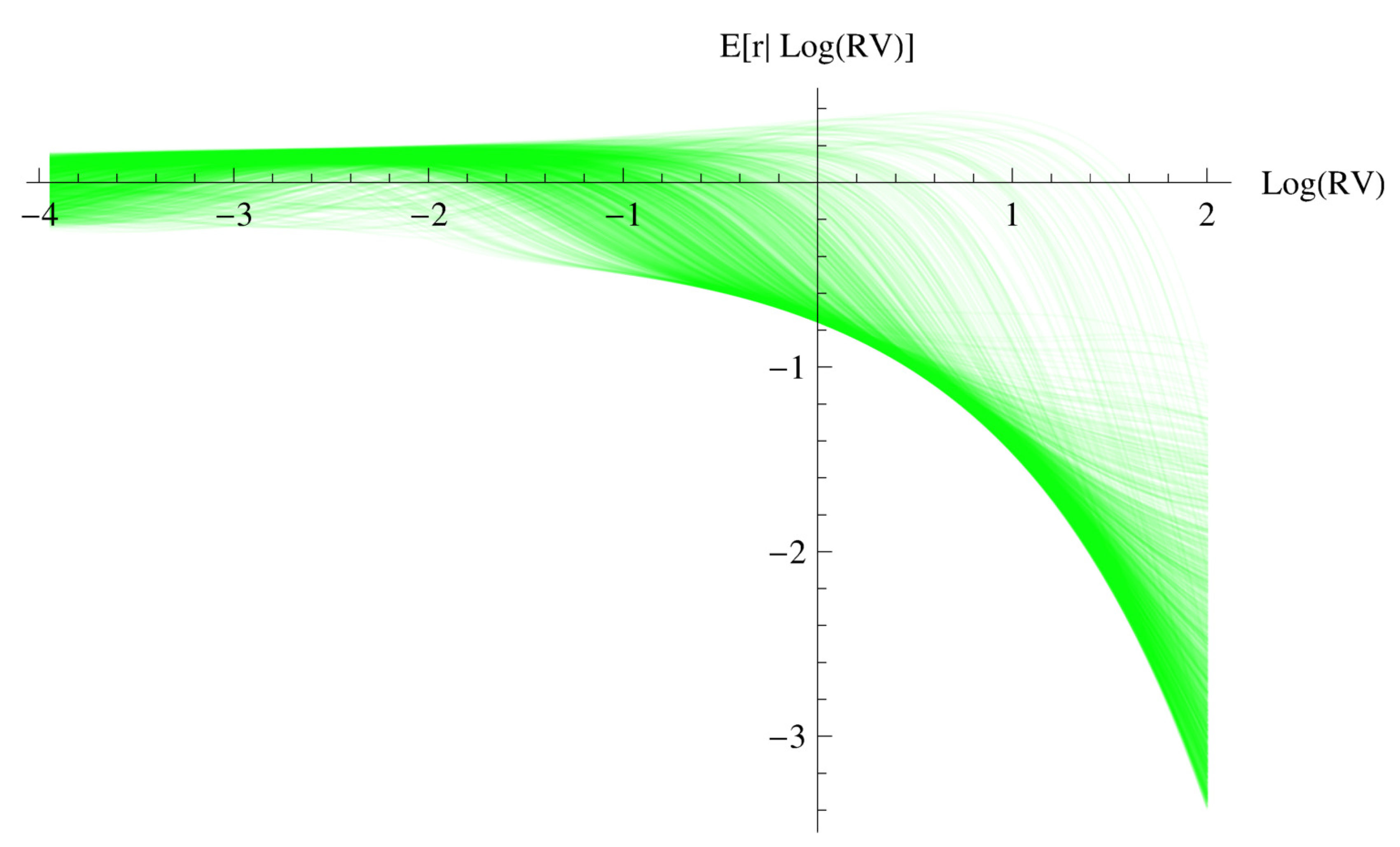
Figure 4.
Expected excess return given log realized variance for the information set where volatility is low. This figure displays the expected excess return and 0.90 density intervals as a function of conditional on the information set , , which is a low volatility period. The expected log-realized volatility based on the model is blue, while the actual log-realized volatility for is the black vertical line.

Figure 5.
Expected excess return given log realized variance for the information set where volatility is near its average level. This figure displays the expected excess return and 0.90 density intervals as a function of conditional on regressors in the information set from , , which is an average volatility period. The expected log-realized volatility based on the model is blue while the actual log-realized volatility for is the black vertical line.

Figure 6.
Expected excess return given log realized variance for the information set where volatility is high. This figure displays the expected excess return and 0.90 density intervals as a function of conditional on regressors in the information set from , , which is a high volatility period. The expected log-realized volatility based on the model is blue while the actual log-realized volatility for is the black vertical line.

Figure 7.
Expected excess return given for various periods. This figure displays the expected excess return as a function of conditional on regressors taken from “Low Log-RV”, , “Average Log-RV” and “High Log-RV”.
Figure 7.
Expected excess return given for various periods. This figure displays the expected excess return as a function of conditional on regressors taken from “Low Log-RV”, , “Average Log-RV” and “High Log-RV”.

Figure 8.
Time series of equity risk premium.

Figure 9.
Expected excess return when volatility feedback is zero.

Figure 10.
Quantiles of excess returns given for the parametric model. This figure displays the quantiles of the distribution of excess returns conditional on for the parametric model. The green dotted line is the expected excess return given .
Figure 10.
Quantiles of excess returns given for the parametric model. This figure displays the quantiles of the distribution of excess returns conditional on for the parametric model. The green dotted line is the expected excess return given .

Figure 11.
Quantiles of excess returns given for low volatility. This figure displays the quantiles of the distribution of excess returns conditional on for , . The green dotted line is the expected excess return given .
Figure 11.
Quantiles of excess returns given for low volatility. This figure displays the quantiles of the distribution of excess returns conditional on for , . The green dotted line is the expected excess return given .

Figure 12.
Quantiles of excess returns given for average volatility. This figure displays the quantiles of the distribution of excess returns conditional on for , . The green dotted line is the expected excess return given .
Figure 12.
Quantiles of excess returns given for average volatility. This figure displays the quantiles of the distribution of excess returns conditional on for , . The green dotted line is the expected excess return given .

Figure 13.
Quantiles of excess returns given for high volatility. This figure displays the quantiles of the distribution of excess returns conditional on for , . The green dotted line is the expected excess return given .
Figure 13.
Quantiles of excess returns given for high volatility. This figure displays the quantiles of the distribution of excess returns conditional on for , . The green dotted line is the expected excess return given .
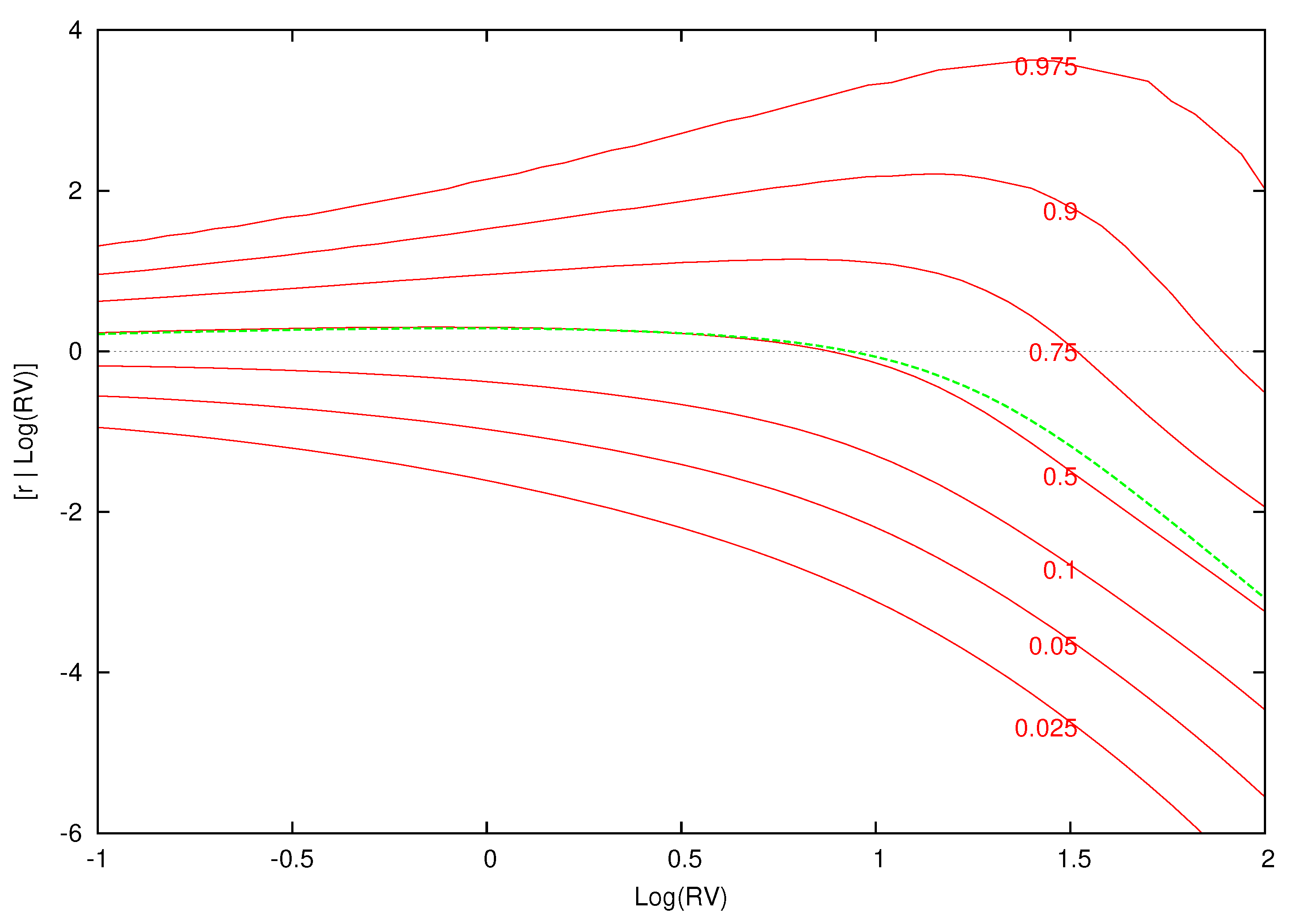
Figure 14.
Predictive density for for low volatility , .

Figure 15.
Predictive density for for average volatility , .

Figure 16.
Predictive density for for high volatility , .

Figure 17.
Posterior means of and .

Figure 18.
Posterior means of and .


Table 1.
Summary statistics.
| Mean | Variance | Skewness | Kurtosis | Min | Max | |
|---|---|---|---|---|---|---|
| 0.0514 | 0.3884 | −0.4047 | 10.0461 | −4.0710 | 4.1630 | |
| 0.3907 | 1.3474 | 9.7037 | 119.5948 | 0.0000 | 17.3300 | |
| 0.3790 | 0.5611 | 7.0305 | 69.4529 | 0.0116 | 11.3000 | |
| −1.5602 | 0.8846 | 0.8051 | 4.2910 | −4.4595 | 2.4245 | |
| 0.2296 | 1.0789 | 0.0030 | 2.6856 | −2.4080 | 2.8580 |
This table reports summary statistics for the monthly data on excess returns and monthly realized volatility . Data is from January 1885–December 2011 giving 1519 observations.
Table 2.
Parametric model estimates.
| Mean | 0.95 Density Interval | |
|---|---|---|
| 0.1922 | (0.1672, 0.2171) | |
| −0.2801 | (−0.3895, −0.1748) | |
| 1.0177 | (0.9460, 1.0962) | |
| −0.3319 | (−0.4151, −0.2470) | |
| 0.3766 | (0.3179, 0.4329) | |
| 0.4505 | (0.3817, 0.5180) | |
| −0.1518 | (−0.1842, −0.1170) | |
| 0.1258 | (0.0680, 0.1861) | |
| 0.3981 | (0.3702, 0.4278) |
This table reports posterior summary statistics for the parametric model:
© 2018 by the authors. Licensee MDPI, Basel, Switzerland. This article is an open access article distributed under the terms and conditions of the Creative Commons Attribution (CC BY) license (http://creativecommons.org/licenses/by/4.0/).
Share and Cite
MDPI and ACS Style
Jensen, M.J.; Maheu, J.M. Risk, Return and Volatility Feedback: A Bayesian Nonparametric Analysis. J. Risk Financial Manag. 2018, 11, 52. https://doi.org/10.3390/jrfm11030052
AMA Style
Jensen MJ, Maheu JM. Risk, Return and Volatility Feedback: A Bayesian Nonparametric Analysis. Journal of Risk and Financial Management. 2018; 11(3):52. https://doi.org/10.3390/jrfm11030052
Chicago/Turabian StyleJensen, Mark J., and John M. Maheu. 2018. "Risk, Return and Volatility Feedback: A Bayesian Nonparametric Analysis" Journal of Risk and Financial Management 11, no. 3: 52. https://doi.org/10.3390/jrfm11030052