3.2. Precipitation Anion Chemistry
Cl
− concentrations were as high as 1.2 mM, with the average value only 0.03 mM. The days that the three highest Cl
− concentrations occurred were 30 December 2010, 18 January 2011, and 1 February 2011, when rain samples turned to ice prior to collection. These extremely high winter Cl
− values may be due, at least in part, to the nearby addition of road de-icing salt around The Ohio State University campus, and thus may be contaminated. However, we have included them in the data set. A statistical analysis using Pearson correlations was done using the day of year, precipitation amount, air temperature, Cl
−, NO
3−, and SO
42− (
Table 1). Significant relationships were noted if the variables had a
p-value < 0.05. Cl
− concentrations in precipitation had a significant negative relationship with air temperature, and a significant positive correlation with NO
3− and SO
42−.
NO3− concentrations were as high as 0.34 mM, which occurred on 8 April 2011, with an average NO3− concentration of 0.04 mM. A significant negative correlation existed between NO3− and precipitation amount, with a positive correlation between SO42− and Cl−.
SO42− concentrations ranged as high as 0.61 mM, which occurred on 23 October 2010, with an average concentration of 0.03 mM. A significant relationship was seen between SO42− and precipitation amount, Cl−, and NO3−. A negative correlation existed between precipitation amount and SO42−. Sulfate concentrations were positively correlated with Cl− and NO3−. These data were consistent with increased precipitation amounts decreasing, or diluting out, the anion concentrations.
3.3. Reservoir Water Anion Chemistry
The Pearson correlation coefficients of significance with a
p-value <0.05 for reservoir data are presented in
Table 2,
Table 3,
Table 4 and
Table 5. All variables that were significantly correlated varied from reservoir to reservoir. Many similarities did occur between the previously mentioned connected/comparable systems of Griggs-O’Shaughnessy and Alum-Hoover. A significant positive correlation occurred between Cl
− and SO
42− in both reservoir systems of flow-through and lacustrine.
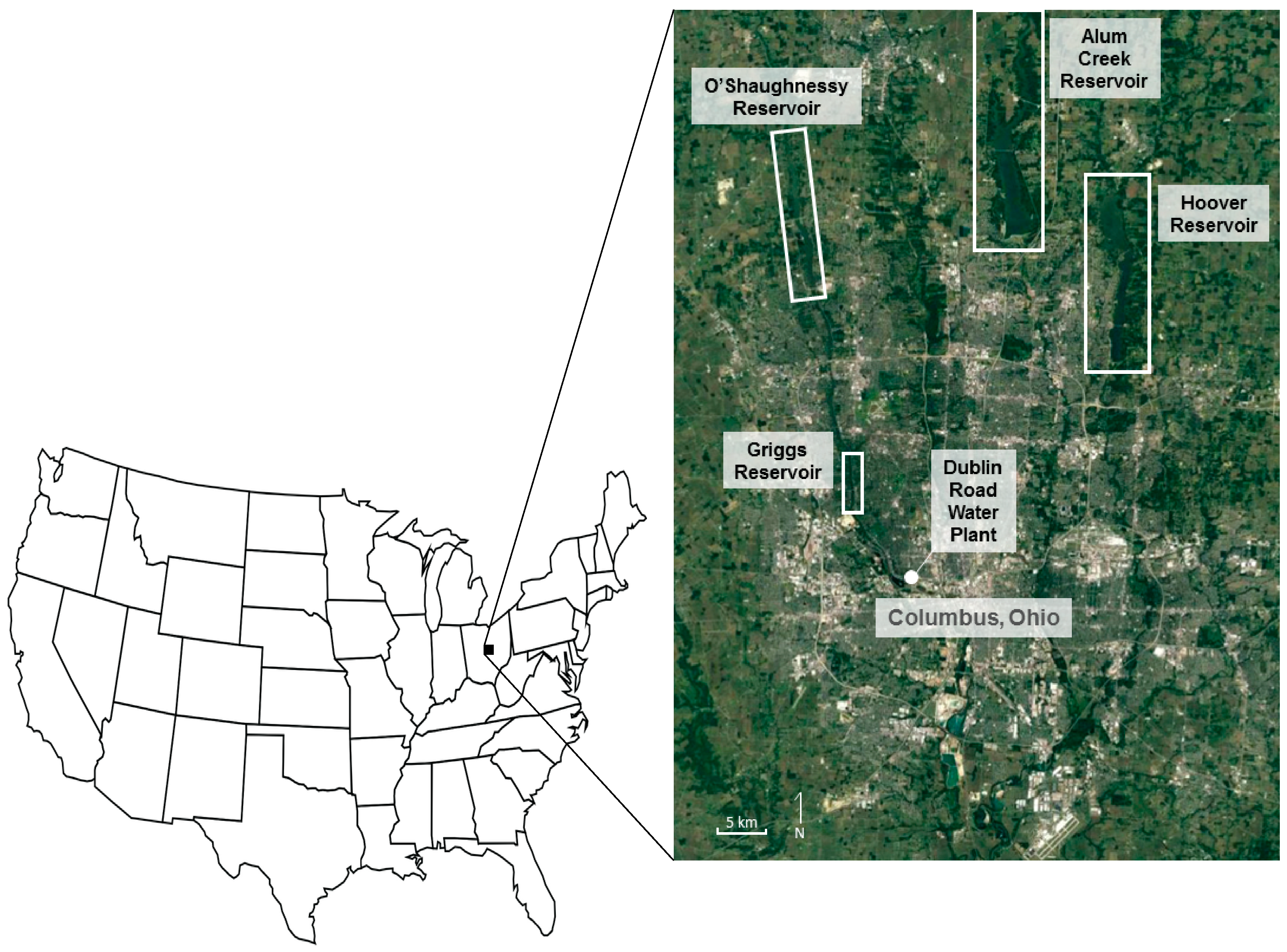
As noted above, the Griggs-O’Shaughnessy (henceforth G-O) system functions more like a riverine system, while the Alum-Hoover (henceforth A-H) system is more like a lacustrine system [
16]. This difference is reflected in most of the anion data. The G-O system is much more variable through time with a shorter residence time of 26 days and 5× the drainage area of A-H; signifying more runoff, less mixing, and acting as a plug flow reactor model (PFR) to control anion concentrations [
16]. The A-H system has relatively constant concentrations with a longer residence time of 152 days and a smaller drainage area; resulting in more mixing with less runoff to describe a completely mixed flow reactor model (CMFR) [
16].
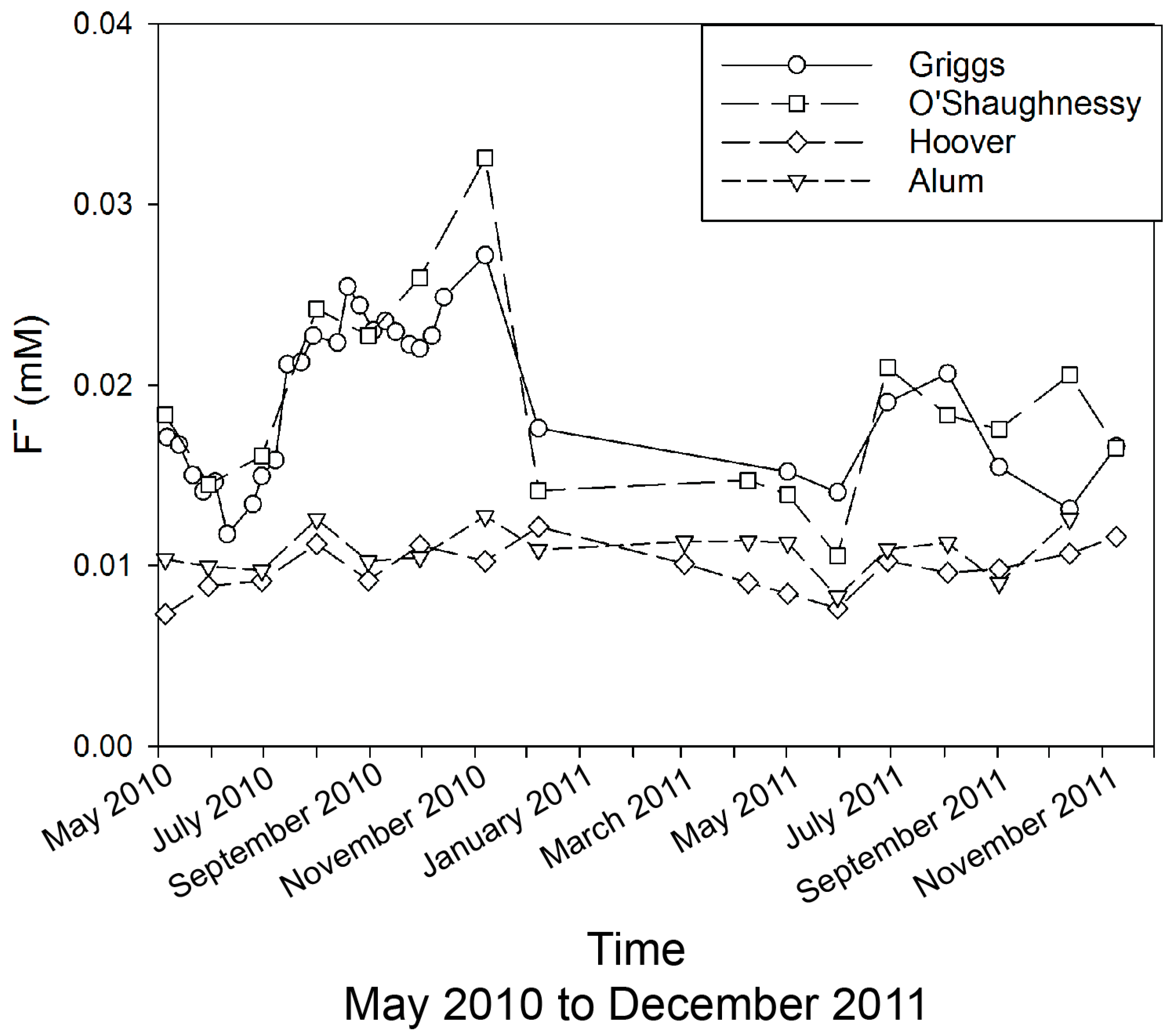
The F
− concentrations in the reservoir water are all below 34 µM, with G-O values being as much as 2× to 3× higher than the A-H values through most of the year (
Figure 3). The G-O shows higher concentrations in the late summer/fall, with the highest concentrations in July–November of 2011 during times of higher precipitation. These F
− values, especially those of the A-H system, are within the range and close to the mean values of 13 µM and 16 µM, for South Asia and United Kingdom rivers, respectively [
24,
25], suggesting potential baseline concentrations for central Ohio. The reason for the higher concentrations in G-O is not known. It should be noted that there is a difference in headwater lithologies between G-O and A-H, where G-O is of limestone/dolomites and shale, while A-H consists primarily of shale. For example, the mineral fluorite (CaF
2) is known to be associated with Silurian aged dolomites in Ohio [
26].
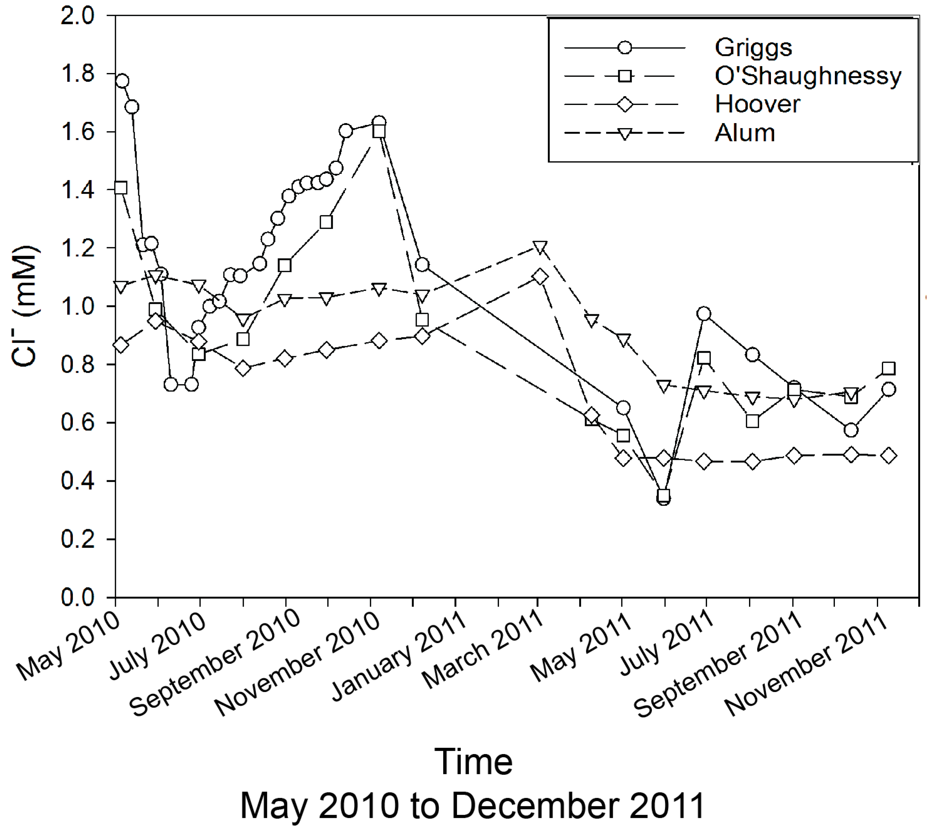
The Cl
− concentrations in these reservoirs ranged from <0.1 to 1.8 µM, with generally slightly lower concentrations in the A-H system (
Figure 4). The mean Cl
− value in “natural” river systems in North America has been determined to be ~0.2 mM, while the “actual” mean is 0.26 mM [
27]. The majority of the reservoir values are above these concentrations, indicating above average input of Cl
− into these systems. This Cl
− comes from the addition of road de-icing salt [
5,
28]. However, the highest concentrations are in the G-O systems, rising through the summer into early winter, and in the late spring/early summer period. Although Gardner and Carey [
28] have documented a continual flux of de-icing salt from major highways in Columbus throughout the year, it is unlikely that this is the primary source of Cl
− to these reservoirs in the summer months. The direct source of this Cl
− is unknown, but reservoir Cl
− systematics could reflect a dilution or concentration depending on precipitation amounts.
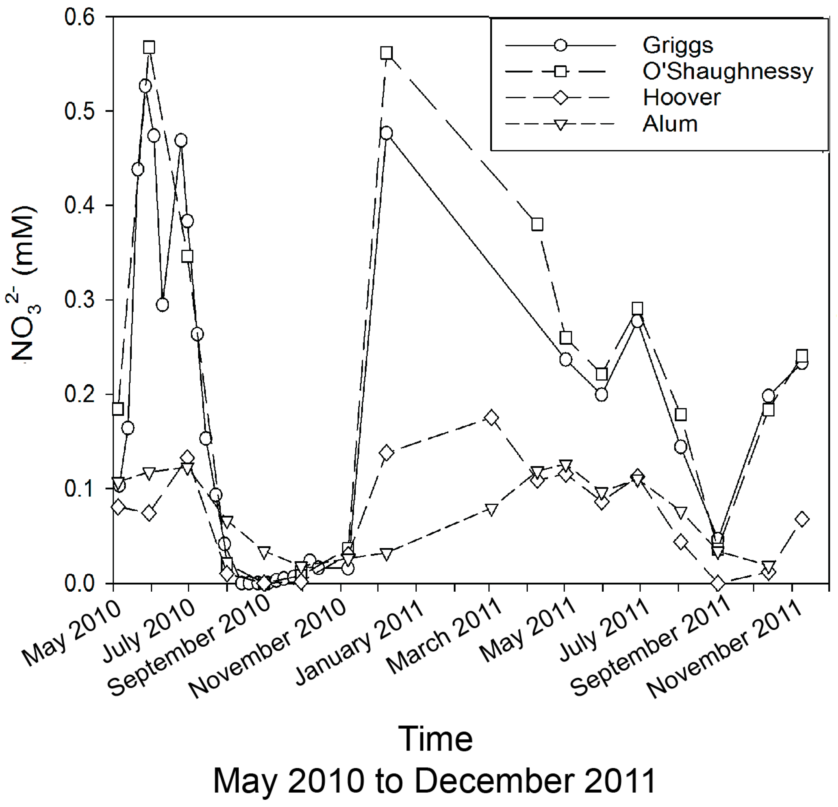
Nitrate concentrations in the A-H fluctuate around 0.1 mM, with lower concentrations in the late summer/early fall that we attribute to biological uptake within the watershed, possibly in the reservoirs themselves (
Figure 5). The G-O data show similar decreases in the summer/fall to concentrations observed in A-H, but the G-O system has early summer and winter concentrations approaching 0.6 mM (
Figure 5). The high values in the spring are probably due to runoff from recently fertilized agricultural lands in the northern part of the watershed, but it is unclear what the source of higher winter values are. During the winter increase in NO
3−, both the Cl
− and SO
42− values are decreasing, implying different sources of these solutes to these reservoirs. Previous work in central Ohio streams/rivers affected by agricultural activities has demonstrated increases as large as 90% from summer NO
3− lows to spring NO
3− highs [
5]. Nitrate concentrations as high as 0.67 mM and values as low as 0.04 mM have recently been observed in agriculturally dominated streams in central Ohio [
5]. This range of NO
3− values is similar to those observed by us in these reservoir waters.
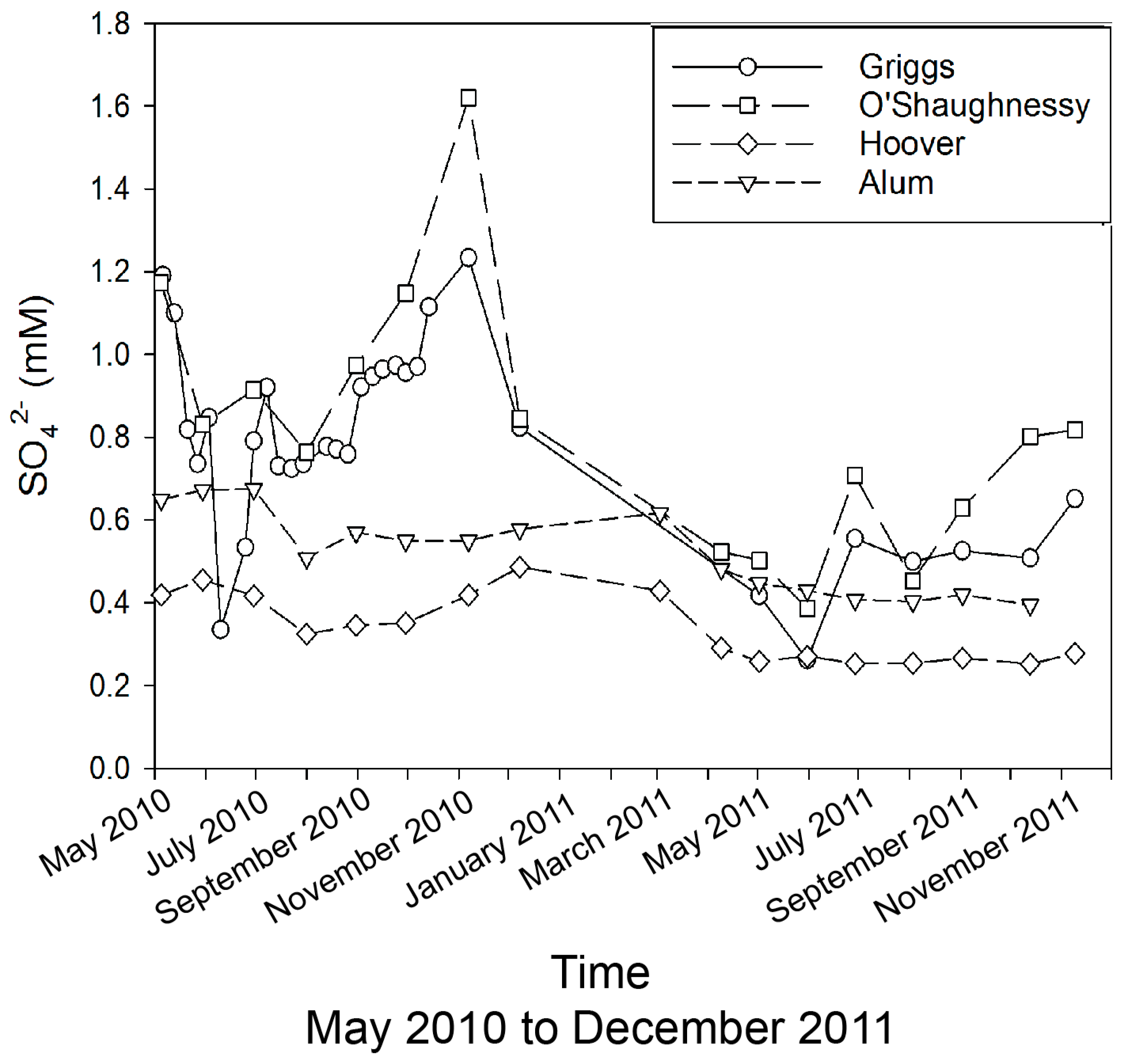
Sulfate concentrations show a similar pattern to Cl
−. In general, the G-O system has higher concentrations with ~2-fold variations, while the A-H system has lower concentrations (0.3–0.6 mM) (
Figure 6). The average North American river SO
42− concentration is 0.19 mM, so even the A-H waters have relatively elevated values, while the highest G-O values of ~1.6 mM are close to an order of magnitude above the North American mean. The G-O SO
42− time series closely resembles the Cl
− pattern, perhaps suggesting similar sources or similar processes controlling their distributions.
Both the Griggs-O’Shaughnessy and Hoover-Alum followed similar trends in anion concentrations over time. Chloride and sulfate concentrations were higher in May 2010, decreased during June 2010, and increased steadily until November 2010. This was followed by a steady decrease in concentrations through June 2011. Concentrations rose in July 2011, and then Cl− decreased, while SO42− remained relatively constant through the rest of the time series. Nitrate increased in June 2010 and then decreased corresponding with decreases in Cl− and SO42−. Low NO3− concentrations occurred through November 2010, with a spike in December 2010. Then NO3− values steadily decreased until September 2011, with a minor increase into October–November 2011. Hoover and Alum Creek Reservoirs had relatively constant concentrations of SO42− and NO3− throughout the study with minimal fluctuation of SO42− concentrations of <0.1 mM and with NO3− concentrations fairly constant. The concentrations of Cl- in Alum Creek Reservoir changed by 0.3 mM throughout the time period, and Cl− reached its peak of ~1.2 mM in March 2011. The Cl− concentrations continually decrease through November 2011. In the Hoover Reservoir, Cl− values remained constant until December 2010 and increased by March 2011. Hoover Cl− concentrations decreased to their lowest level in July 2011, and by August 2011, concentrations returned to the previous Cl− concentration observed in June 2011.
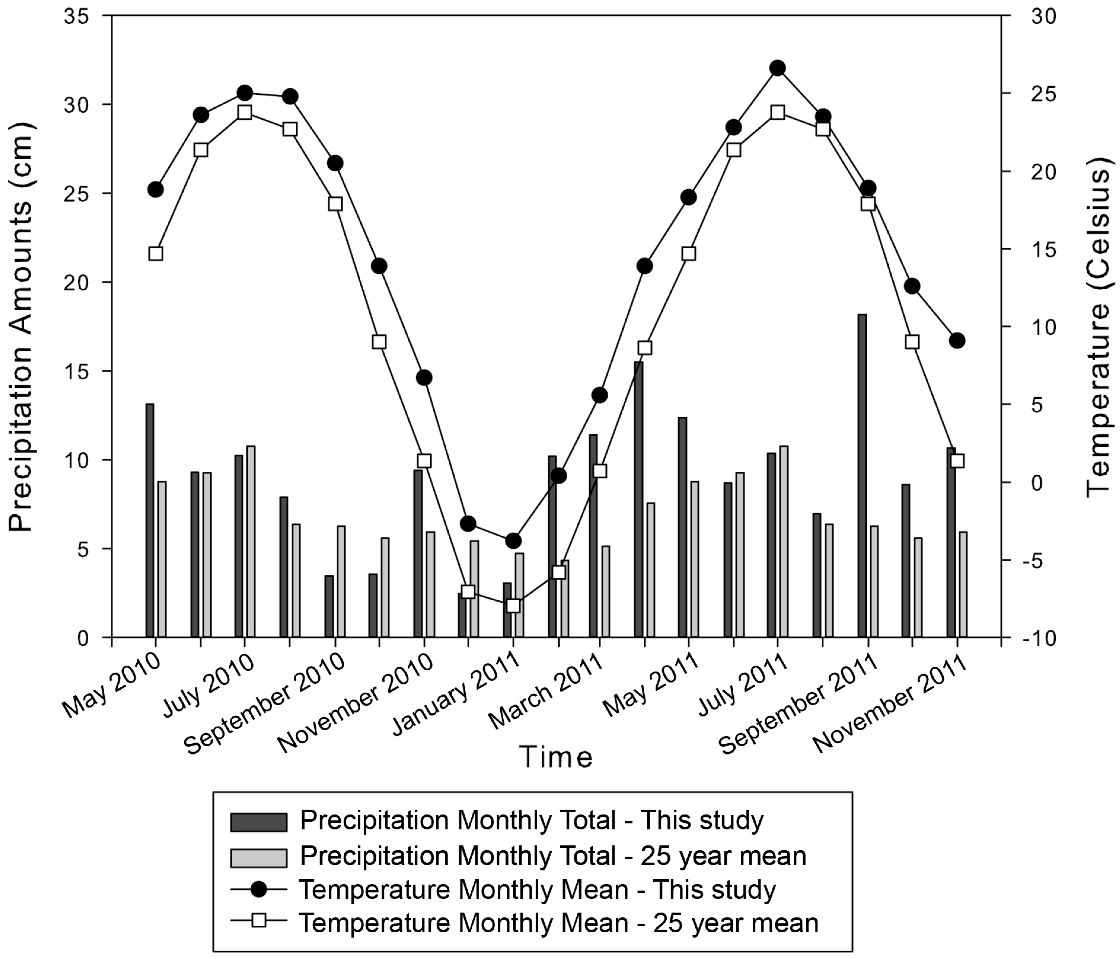
Reservoir management and water supply dynamics are important in order to anticipate water resources availability [
29]. Higher anion concentrations could signify lower reservoir volumes through evapoconcentration and/or water consumption. Precipitation amounts were near the 25-year average during this period in 2010. Reservoir waters of lower anion concentrations occurred during June–November 2011, which likely indicates that higher precipitation volumes diluted reservoir anion concentrations. We suggest that the observed reservoir behavior that occurred in 2010 was due to evaporation, while in 2011, increased precipitation amounts diluted anion concentrations. Normally, conservative elements such as Cl
− can be utilized to help determine evaporation effects, but the high Cl
− concentrations in these reservoir waters and the lack of knowledge about its sources make this more challenging. This aspect of the systems’ anion geochemistry complicates discerning between reservoir evaporative loss and variations in precipitation sources.
3.4. Residential Tap Waters
Over the time of this investigation, Cl− and SO42− followed similar trends, while NO3− and F− varied together as well. Chloride concentrations increased to 6.9 mM on 6 February 2011 with an average concentration of 1.5 mM. The highest SO42− concentration of 1.8 mM occurred on 24 October 2010 with an average concentration of 1.2 mM. Fluoride and nitrate concentrations were minimal, <0.05 mM, with higher nitrate levels of ~0.05 mM occurring in June 2010, December 2010, and January 2011.
Pearson correlations were calculated for the tap water samples (
Table 6). Significant positive correlations existed between day of year–SO
42−, F
−–Cl
−, F
−–NO
3−, F
−–SO
42−, Cl
−–NO
3−, and Cl
−–SO
42−. Significant negative relationships occurred between day of year–Cl
−, day of year–NO
3−, temperature–F
−, temperature–Cl
−, temperature–NO
3−, and temperature–SO
42−. Chloride and nitrate had lower concentrations later in the calendar year, while SO
42− had higher concentrations later in the year. The negative correlations with temperature indicate that as the air temperature increases, solute concentrations decrease. Solute–solute correlations of F
− and Cl
− with NO
3−, SO
42−, and Cl
− have positive correlations, demonstrating a co-variance.
3.5. Anion Comparison of Precipitation to Reservoir To Tap
Plots to compare over time the four anionic species from each of the three water types (precipitation ➔ reservoir ➔ tap) are shown in
Figure 7. The F
−, Cl
−, NO
3−, and SO
42− concentrations in the precipitation were all equal or lower than in the reservoirs with a few exceptions. Seemingly anomalously high NO
3− concentrations in precipitation collected in April 2011 are thought to be due to a local effect near the collection site. In general, the tap water has concentrations similar or lower than the reservoir. Not surprisingly, the tap has in most cases 2× higher F
− than the reservoir water, as F
− is being added as an anti-tooth decay agent during the treatment process. Our highest observed F
− value is very similar to that reported by the City of Columbus for tap water (~62 µM) [
30]. At most times, the SO
42− concentration in the tap water were greater than the reservoir value. This should be expected, given the fact that alum (Al-SO
4 salts) is used to treat the water before distribution. In most cases, the Cl
− in the tap water was higher than the reservoirs (
Figure 7B), but this difference is rather small (~0.1–0.2 mM). The rather large difference in January to March 2011 may be because of an extensive ice cover on the reservoirs themselves. The reservoirs were not sampled during this time, while the tap water was. Here, the tap water may well represent the reservoir Cl
− concentrations due to the influx for Cl
− from the local highway de-icing and potentially other anthropogenic activities, but we have no reservoir water to substantiate this hypothesis.


