
Trade-Off and Synergy among Ecosystem Services in the Guanzhong-Tianshui Economic Region of China

Abstract
:1. Introduction
2. Method
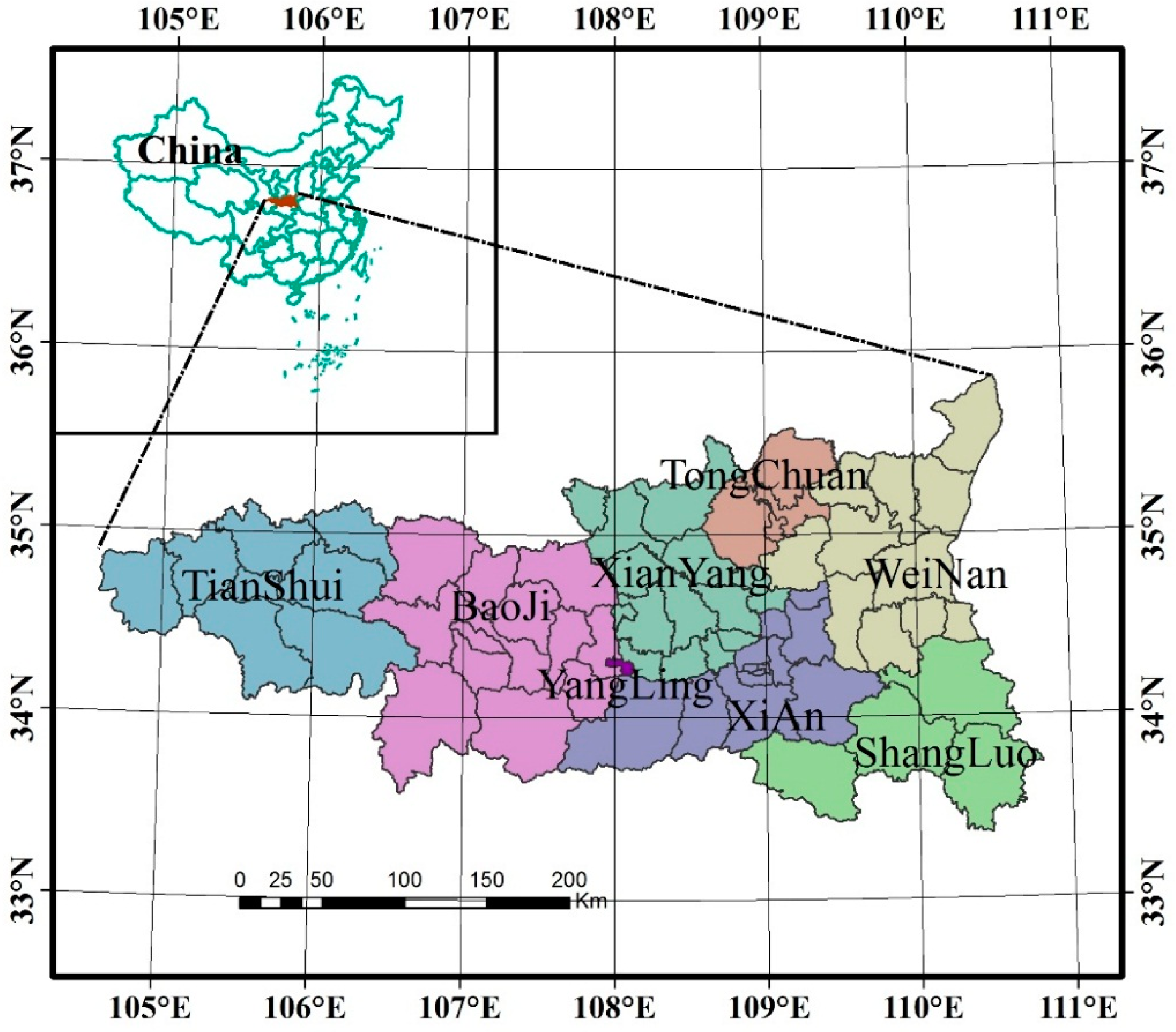
2.1. Study Area

2.2. Data Source

| Required Data | Soil and Water Conservation | Water Interception | Carbon Sequestration | Agricultural Production | Water Yield | Data Source |
|---|---|---|---|---|---|---|
| Land-Use Map | ▬ | ▬ | Landsat TM | |||
| DEM | ▬ | Topographic Map of 1:50,000 | ||||
| Soil Type | ▬ | Agricultural Sector | ||||
| Rainfall | ▬ | ▬ | Agricultural Sector | |||
| Temperature | ▬ | Agricultural Sector | ||||
| Evaporation | ▬ | ▬ | Meteorological Department | |||
| Solar Radiation | ▬ | Meteorological Department | ||||
| Administrative Map | ▬ | ▬ | ▬ | Civil Affairs | ||
| Grain Production | ▬ | Statistical Yearbook |
2.3. Methods of Analysis
2.3.1. Water Yield
2.3.2. Carbon Sequestration
2.3.3. Water Interception
2.3.4. Soil Conservation
2.3.5. Agricultural Production
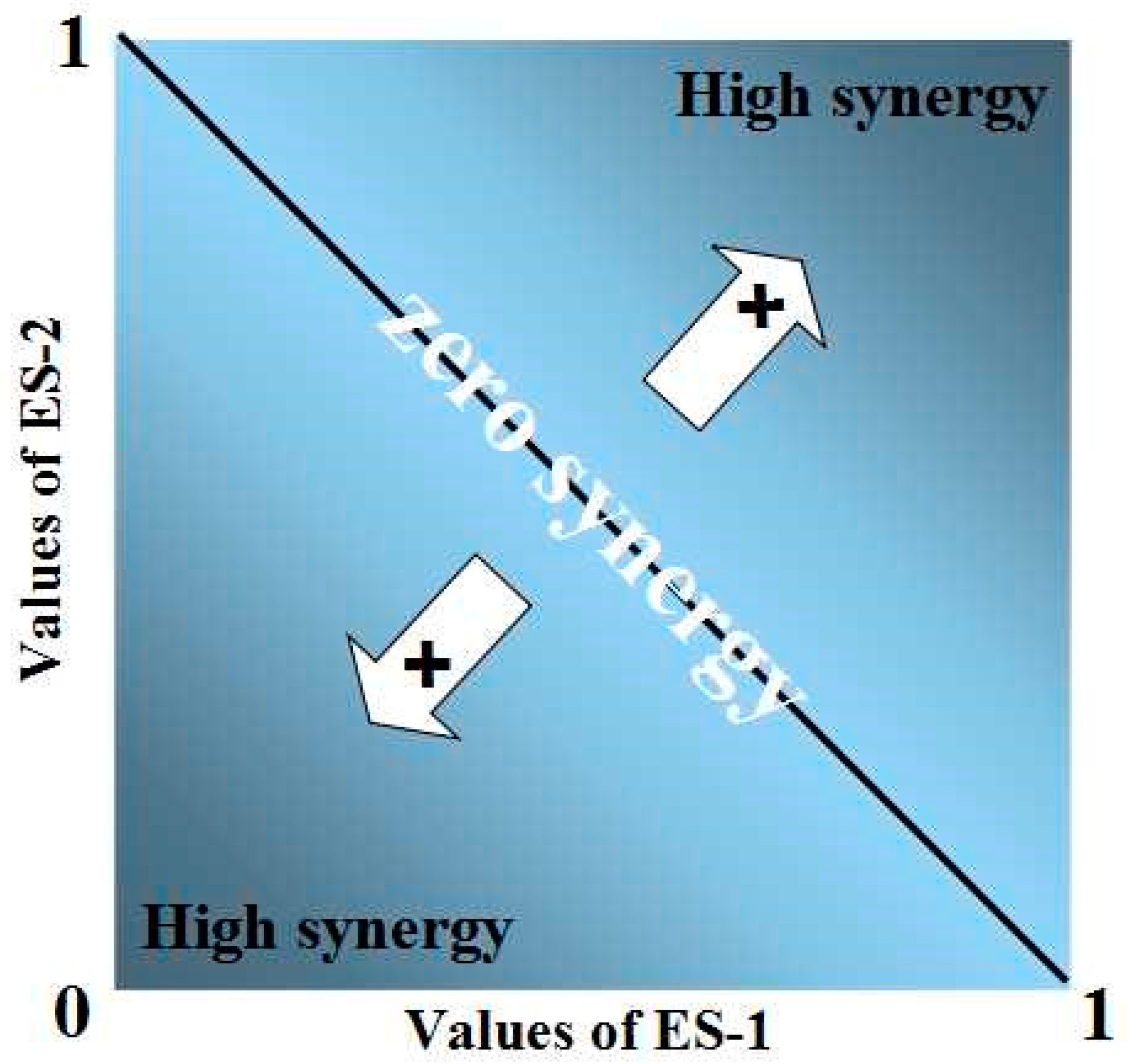
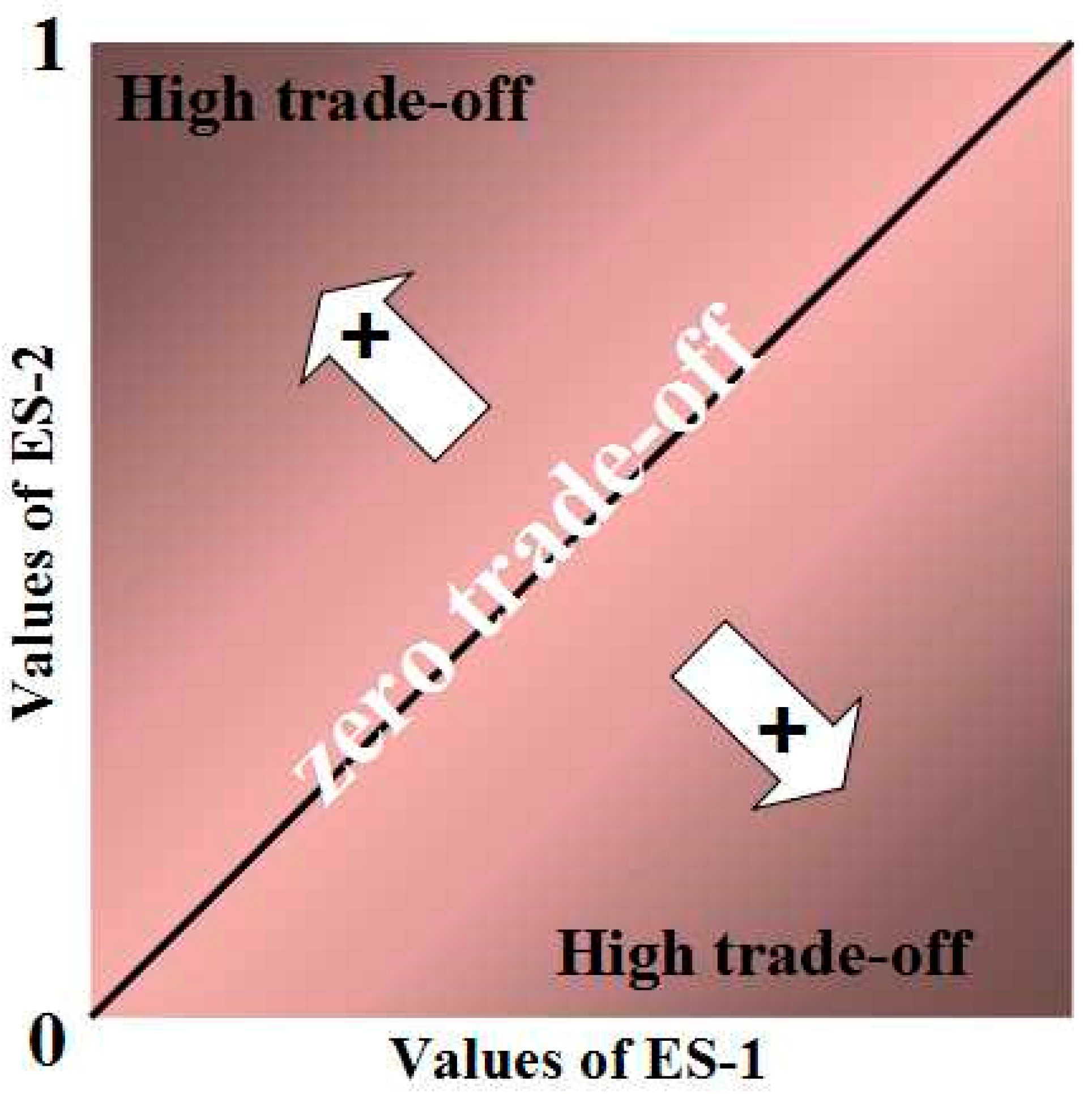
2.3.6. Finding Out and Quantification of Trade-Offs and Synergies


3. Results
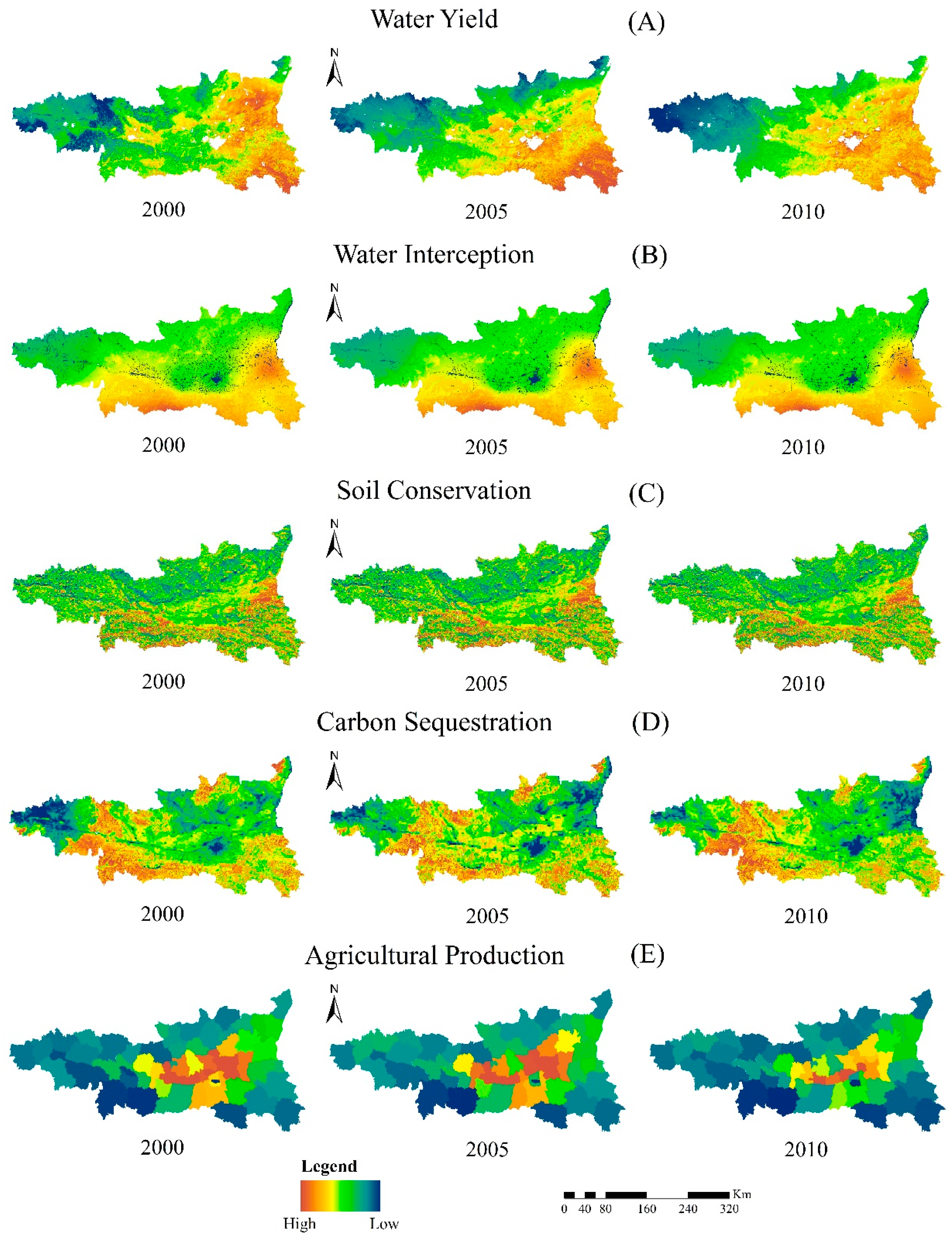
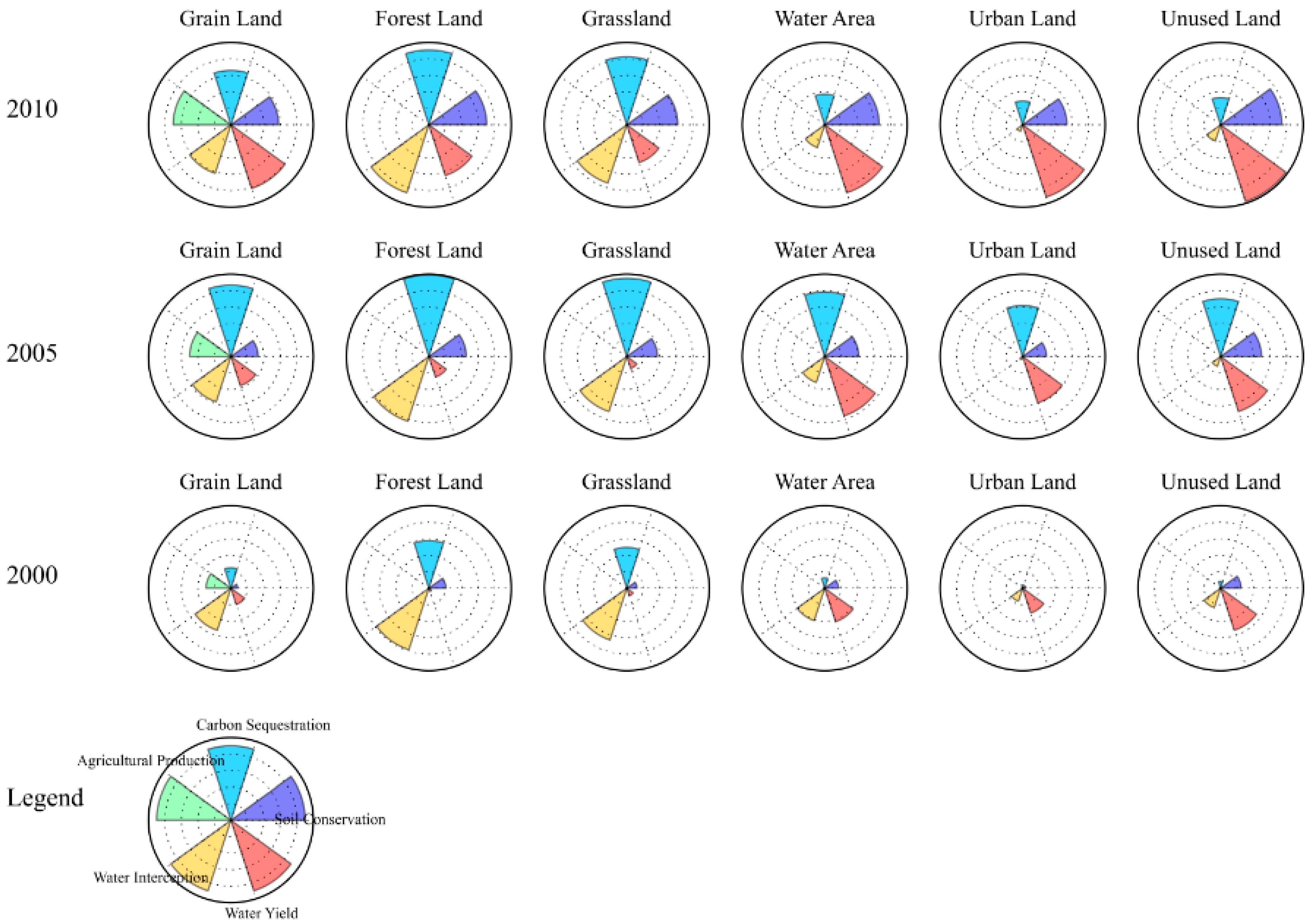
3.1. Temporal and Spatial Distribution Characteristics of Ecosystem Services

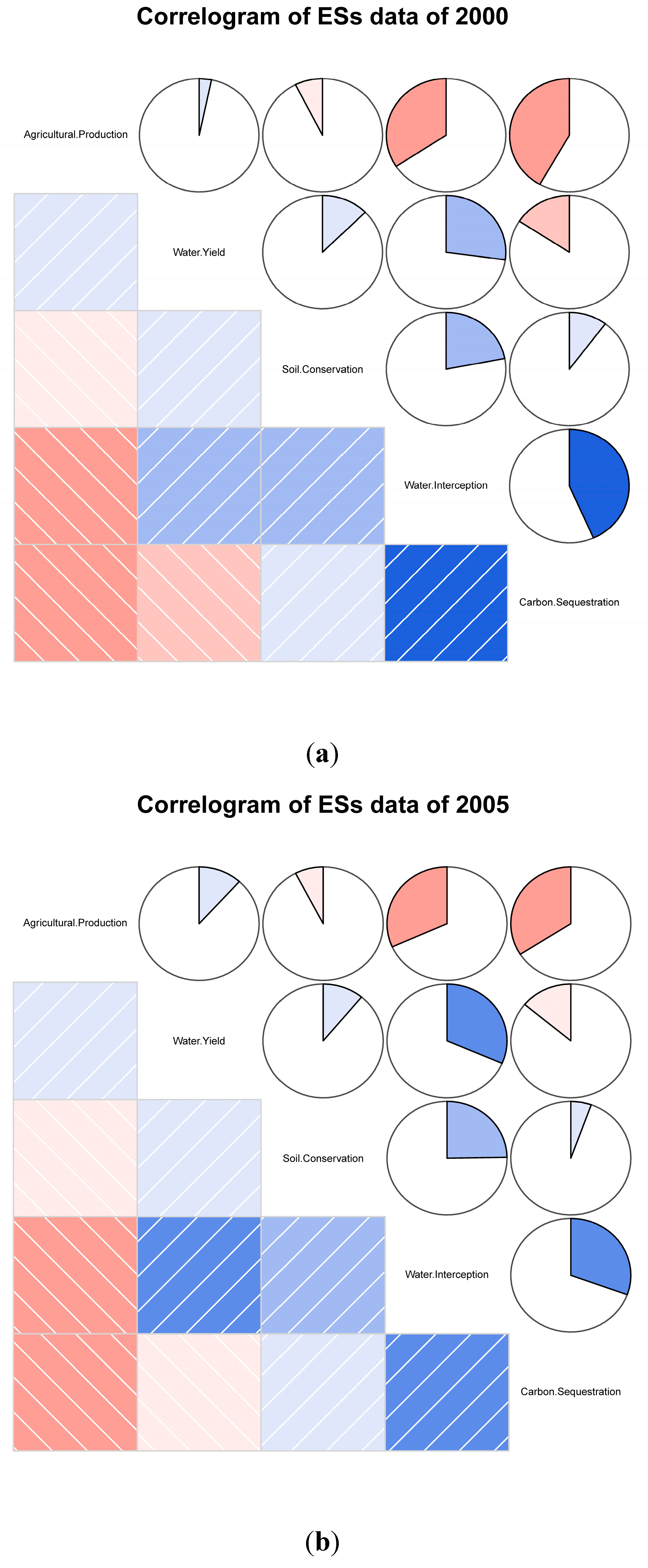
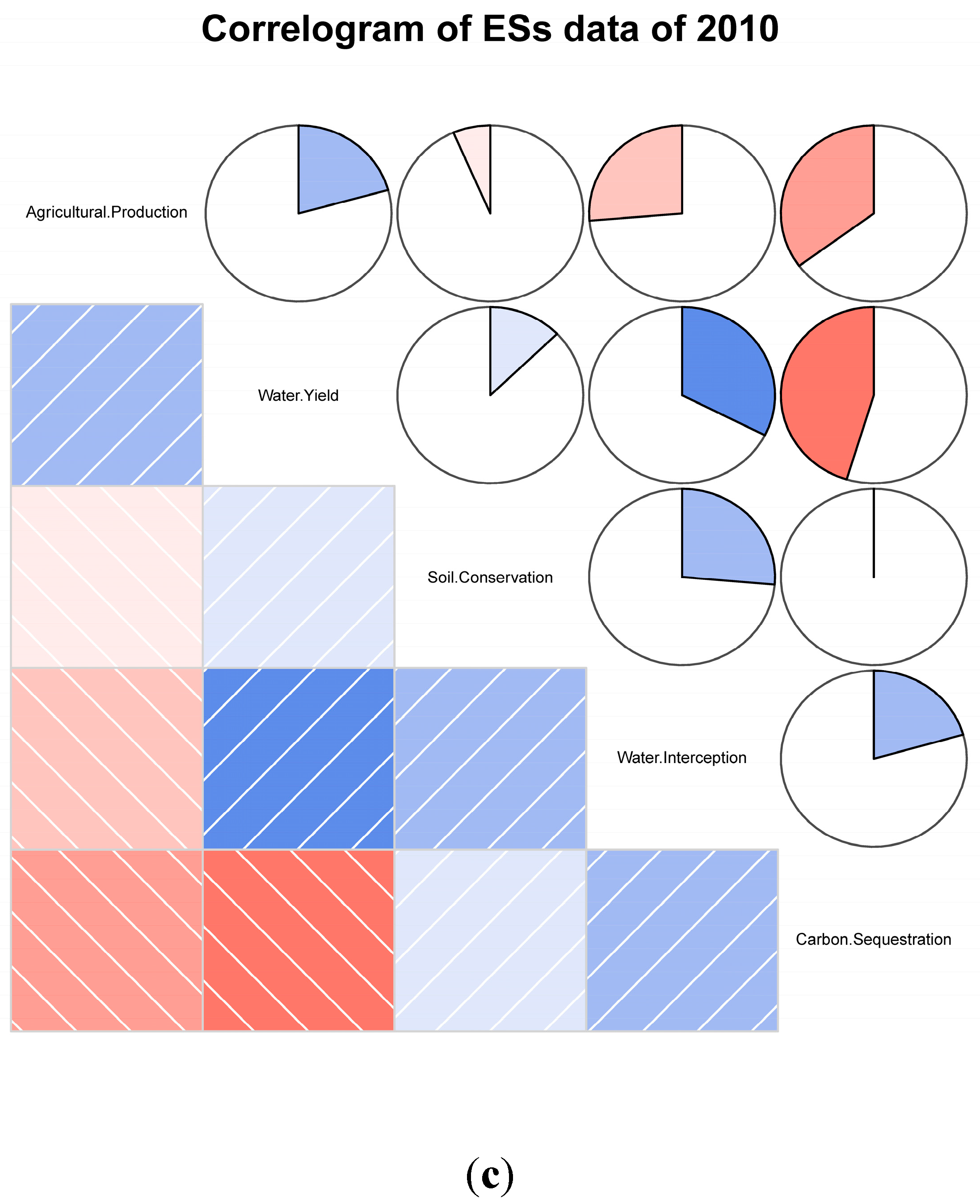
3.2. Interactions among Ecosystem Services
3.3. Quantification of Trade-Offs and Synergies
4. Discussion


| Water Yield | Water Interception | Soil Conservation | Carbon Sequestration | Agricultural Production | |
|---|---|---|---|---|---|
| 2010 | |||||
| Water Yield | - | ||||
| Water Interception | 0.29 | - | |||
| Soil Conservation | 0.18 | 0.15 | - | ||
| Carbon Sequestration | 0.19 | 0.27 | 0.13 | - | |
| Agricultural Production | 0.30 | 0.50 | 0.24 | 0.40 | - |
| 2005 | |||||
| Water Yield | - | ||||
| Water Interception | 0.23 | - | |||
| Soil Conservation | 0.20 | 0.15 | - | ||
| Carbon Sequestration | 0.16 | 0.25 | 0.13 | - | |
| Agricultural Production | 0.30 | 0.44 | 0.21 | 0.33 | - |
| 2000 | |||||
| Water Yield | - | ||||
| Water Interception | 0.25 | - | |||
| Soil Conservation | 0.17 | 0.15 | - | ||
| Carbon Sequestration | 0.16 | 0.26 | 0.16 | - | |
| Agricultural Production | 0.27 | 0.45 | 0.21 | 0.34 | - |
5. Conclusions
Acknowledgments
Author Contributions
Conflicts of Interest
References
- Fisher, B.; Turner, R.K.; Morling, P. Defining and classifying ecosystem services for decision making. Ecol. Econ. 2009, 68, 643–653. [Google Scholar] [CrossRef]
- Vitousek, P.M.; Mooney, H.A.; Lubchenco, J.; Melillo, J.M. Human domination of Earth’s ecosystems. Science 1997, 277, 494–499. [Google Scholar] [CrossRef]
- Foley, J.A.; Costa, M.H.; Delire, C.; Ramankutty, N.; Snyder, P. Green surprise? How terrestrial ecosystems could affect earth’s climate. Front. Ecol. Environ. 2003, 1, 38–44. [Google Scholar]
- Daily, G.C.; Polasky, S.; Goldstein, J.; Kareiva, P.M.; Mooney, H.A.; Pejchar, L.; Ricketts, T.H.; Salzman, J.; Shallenberger, R. Ecosystem services in decision making: Time to deliver. Front. Ecol. Environ. 2009, 7, 21–28. [Google Scholar] [CrossRef]
- Kareiva, P.; Watts, S.; McDonald, R.; Boucher, T. Domesticated nature: Shaping landscapes and ecosystems for human welfare. Science 2007, 316, 1866–1869. [Google Scholar] [CrossRef] [PubMed]
- Bai, Y.; Zheng, H.; Ouyang, Z.; Zhuang, C.; Jiang, B. Modeling hydrological ecosystem services and tradeoffs: A case study in Baiyangdian watershed, China. Environ. Earth Sci. 2013, 70, 709–718. [Google Scholar] [CrossRef]
- Aillery, M.; Shoemaker, R.; Caswell, M. Agriculture and ecosystem restoration in South Florida: Assessing trade-offs from water-retention development in the Everglades agricultural area. Am. J. Agric. Econ. 2001, 83, 183–195. [Google Scholar] [CrossRef]
- Backéus, S.; Wikström, P.; Lämås, T. A model for regional analysis of carbon sequestration and timber production. For. Ecol. Manag. 2005, 216, 28–40. [Google Scholar] [CrossRef]
- Phelps, J.; Friess, D.; Webb, E. Win-win REDD+ approaches belie carbon-biodiversity trade-offs. Biol. Conserv. 2012, 154, 53–60. [Google Scholar] [CrossRef]
- Tallis, H.; Polasky, S. Assessing Multiple Ecosystem Services: An integrated tool for the real world. In Natural Capital. Theory and Practice of Mapping Ecosystem Services; Oxford University Press: Oxford, UK, 2011; pp. 34–52. [Google Scholar]
- Kragt, M.E.; Robertson, M.J. Quantifying ecosystem services trade-offs from agricultural practices. Ecol. Econ. 2014, 102, 147–157. [Google Scholar] [CrossRef]
- Dymond, J.R.; Ausseil, A.-G.E.; Ekanayake, J.C.; Kirschbaum, M.U. Tradeoffs between soil, water, and carbon—A national scale analysis from New Zealand. J. Environ. Manag. 2012, 95, 124–131. [Google Scholar] [CrossRef] [PubMed]
- Goldstein, J.H.; Caldarone, G.; Duarte, T.K.; Ennaanay, D.; Hannahs, N.; Mendoza, G.; Polasky, S.; Wolny, S.; Daily, G.C. Integrating ecosystem-service tradeoffs into land-use decisions. Proc. Natl. Acad. Sci. USA 2012, 109, 7565–7570. [Google Scholar] [CrossRef] [PubMed]
- Hicks, C.C. How do we value our reefs? Risks and tradeoffs across scales in “biomass-based” economies. Coast. Manag. 2011, 39, 358–376. [Google Scholar] [CrossRef]
- Hicks, C.C.; Graham, N.A.; Cinner, J.E. Synergies and tradeoffs in how managers, scientists, and fishers value coral reef ecosystem services. Glob. Environ. Chang. 2013, 23, 1444–1453. [Google Scholar] [CrossRef]
- Jindal, R.; Kerr, J.M.; Ferraro, P.J.; Swallow, B.M. Social dimensions of procurement auctions for environmental service contracts: Evaluating tradeoffs between cost-effectiveness and participation by the poor in rural Tanzania. Land Use Policy 2013, 31, 71–80. [Google Scholar] [CrossRef]
- Lester, S.E.; Costello, C.; Halpern, B.S.; Gaines, S.D.; White, C.; Barth, J.A. Evaluating tradeoffs among ecosystem services to inform marine spatial planning. Mar. Policy 2013, 38, 80–89. [Google Scholar] [CrossRef]
- Meehan, T.D.; Gratton, C.; Diehl, E.; Hunt, N.D.; Mooney, D.F.; Ventura, S.J.; Barham, B.L.; Jackson, R.D. Ecosystem-service tradeoffs associated with switching from annual to perennial energy crops in riparian zones of the US Midwest. PLoS ONE 2013. [Google Scholar] [CrossRef] [PubMed]
- Raudsepp-Hearne, C.; Peterson, G.D.; Bennett, E. Ecosystem service bundles for analyzing tradeoffs in diverse landscapes. Proc. Natl. Acad. Sci. USA 2010, 107, 5242–5247. [Google Scholar] [CrossRef] [PubMed]
- Rodríguez, J.P.; Beard, T.D.; Bennett, E.M.; Cumming, G.S.; Cork, S.J.; Agard, J.; Dobson, A.P.; Peterson, G.D. Trade-offs across space, time, and ecosystem services. Available online: http://www.ecologyandsociety.org/vol11/iss1/art28/ (accessed on 28 October 2015).
- Swallow, B.M.; Sang, J.K.; Nyabenge, M.; Bundotich, D.K.; Duraiappah, A.K.; Yatich, T.B. Tradeoffs, synergies and traps among ecosystem services in the Lake Victoria basin of East Africa. Environ. Sci. Policy 2009, 12, 504–519. [Google Scholar] [CrossRef]
- Viglizzo, E.F.; Frank, F.C. Land-use options for Del Plata Basin in South America: Tradeoffs analysis based on ecosystem service provision. Ecol. Econ. 2006, 57, 140–151. [Google Scholar] [CrossRef]
- Acreman, M.; Harding, R.; Lloyd, C.; McNamara, N.; Mountford, J.; Mould, D.; Purse, B.; Heard, M.; Stratford, C.; Dury, S. Trade-off in ecosystem services of the Somerset Levels and Moors wetlands. Hydrol. Sci. J. 2011, 56, 1543–1565. [Google Scholar] [CrossRef]
- Millennium Ecosystem Assessment. Millennium Ecosystem Assessment; Millennium Ecosystem Assessment; Island Press: Washington, DC, USA, 2001. [Google Scholar]
- Bennett, E.M.; Balvanera, P. The future of production systems in a globalized world. Front. Ecol. Environ. 2007, 5, 191–198. [Google Scholar] [CrossRef]
- Butler, J.R.; Wong, G.Y.; Metcalfe, D.J.; Honzák, M.; Pert, P.L.; Rao, N.; van Grieken, M.E.; Lawson, T.; Bruce, C.; Kroon, F.J. An analysis of trade-offs between multiple ecosystem services and stakeholders linked to land use and water quality management in the Great Barrier Reef, Australia. Agric. Ecosyst. Environ. 2013, 180, 176–191. [Google Scholar] [CrossRef]
- Tallis, H.; Kareiva, P.; Marvier, M.; Chang, A. An ecosystem services framework to support both practical conservation and economic development. Proc. Natl. Acad. Sci. USA 2008, 105, 9457–9464. [Google Scholar] [CrossRef] [PubMed]
- Bennett, E.M.; Peterson, G.D.; Gordon, L.J. Understanding relationships among multiple ecosystem services. Ecol. Lett. 2009, 12, 1394–1404. [Google Scholar] [CrossRef] [PubMed]
- Carpenter, S.R.; Mooney, H.A.; Agard, J.; Capistrano, D.; DeFries, R.S.; Díaz, S.; Dietz, T.; Duraiappah, A.K.; Oteng-Yeboah, A.; Pereira, H.M. Science for managing ecosystem services: Beyond the Millennium Ecosystem Assessment. Proc. Natl. Acad. Sci. USA 2009, 106, 1305–1312. [Google Scholar] [CrossRef] [PubMed]
- Boody, G.; Vondracek, B.; Andow, D.A.; Krinke, M.; Westra, J.; Zimmerman, J.; Welle, P. Multifunctional agriculture in the United States. BioScience 2005, 55, 27–38. [Google Scholar] [CrossRef]
- López, E.; Bocco, G.; Mendoza, M.; Duhau, E. Predicting land-cover and land-use change in the urban fringe: A case in Morelia city, Mexico. Landsc. Urban Plan. 2001, 55, 271–285. [Google Scholar] [CrossRef]
- White, C.; Halpern, B.S.; Kappel, C.V. Ecosystem service tradeoff analysis reveals the value of marine spatial planning for multiple ocean uses. Proc. Natl. Acad. Sci. USA 2012, 109, 4696–4701. [Google Scholar] [CrossRef] [PubMed]
- Carreño, L.; Frank, F.; Viglizzo, E. Tradeoffs between economic and ecosystem services in Argentina during 50 years of land-use change. Agric. Ecosyst. Environ. 2012, 154, 68–77. [Google Scholar] [CrossRef]
- Cao, S.; Li, C.; Cao, S.; Peng, Z.; Yang, L. Change in ecosystem service value arising from land consolidation planning in Anhui Province. Asian Agric. Res. 2013, 5, 17–20. [Google Scholar]
- Jia, X.; Fu, B.; Feng, X.; Hou, G.; Liu, Y.; Wang, X. The tradeoff and synergy between ecosystem services in the Grain-for-Green areas in Northern Shaanxi, China. Ecol. Indic. 2014, 43, 103–113. [Google Scholar] [CrossRef]
- Li, D.; Bo, F.; Tao, J. Achievements in and strategies for Grain to Green Program in Hunan Province. Hun. For. Sci. Technol. 2006, 33, 1–5. [Google Scholar]
- Long, H.; Heilig, G.; Wang, J.; Li, X.; Luo, M.; Wu, X.; Zhang, M. Land use and soil erosion in the upper reaches of the Yangtze River: Some socio-economic considerations on China’s Grain-for-Green Programme. Land Degrad. Dev. 2006, 17, 589–603. [Google Scholar] [CrossRef]
- Xu, J.; Yin, R.; Li, Z.; Liu, C. China’s ecological rehabilitation: Unprecedented efforts, dramatic impacts, and requisite policies. Ecol. Econ. 2006, 57, 595–607. [Google Scholar] [CrossRef]
- Budyko, M.I. Climate and Life; Academic Press: Orlando, FL, USA, 1971. [Google Scholar]
- Yuan, J.; Niu, Z.; Wang, C. Vegetation NPP distribution based on MODIS data and CASA model—A case study of northern Hebei Province. Chin. Geograph. Sci. 2006, 16, 334–341. [Google Scholar] [CrossRef]
- Potter, C.S.; Randerson, J.T.; Field, C.B.; Matson, P.A.; Vitousek, P.M.; Mooney, H.A.; Klooster, S.A. Terrestrial ecosystem production: A process model based on global satellite and surface data. Glob. Biogeochem. Cycles 1993, 7, 811–841. [Google Scholar] [CrossRef]
- Wenquan, Z.; Yaozhong, P.; Jinshui, Z. Estimation of net primary productivity of Chinese terrestrial vegetation based on remote sensing. Chin. J. Plant Ecol. 2007, 31, 413–424. [Google Scholar]
- Zhiyuan, R.; Yanfang, Z.; Jing, L. The value of vegetation ecosystem services: A case of Qinling-Daba Mountains. J. Geogr. Sci. 2003, 13, 195–200. [Google Scholar] [CrossRef]
- Jing, L.; Zhiyuan, R. Variations in ecosystem service value in response to land use changes in the Loess Plateau in northern Shaanxi Province, China. Int. J. Environ. Res. 2011, 5, 109–118. [Google Scholar]
- Bagherzadeh, A. Estimation of soil losses by USLE model using GIS at Mashhad plain, Northeast of Iran. Arab. J. Geosci. 2014, 7, 211–220. [Google Scholar] [CrossRef]
- Su, C.; Fu, B.; Wei, Y.; Lü, Y.; Liu, G.; Wang, D.; Mao, K.; Feng, X. Ecosystem management based on ecosystem services and human activities: A case study in the Yanhe watershed. Sustain. Sci. 2012, 7, 17–32. [Google Scholar] [CrossRef]
- Bradford, J.B.; D’Amato, A.W. Recognizing trade-offs in multi-objective land management. Front. Ecol. Environ. 2011, 10, 210–216. [Google Scholar] [CrossRef]
- Gao, Q.; Li, Y.; Wan, Y.; Qin, X.; Jiangcun, W.; Liu, Y. Dynamics of alpine grassland NPP and its response to climate change in Northern Tibet. Clim. Chang. 2009, 97, 515–528. [Google Scholar] [CrossRef]
- Fang, J.; Song, Y.; Liu, H. Vegetation-climate relationship and its application in the division of vegetation zone in China. Acta Bot. Sin. 2002, 44, 1105–1122. [Google Scholar]
- Piao, S.; Fang, J.; He, J. Variations in vegetation net primary production in the Qinghai-Xizang Plateau, China, from 1982 to 1999. Clim. Chang. 2006, 74, 253–267. [Google Scholar] [CrossRef]
- Canqiang, Z.; Wenhua, L.; Biao, Z.; Moucheng, L. Water yield of Xitiaoxi River Basin based on INVEST modeling. J. Resour. Ecol. 2012, 3, 50–54. [Google Scholar] [CrossRef]
- Alvarez, M.; Field, D.B. Tradeoffs among ecosystem benefits: An analysis framework in the evaluation of forest management alternatives. J. For. 2009, 107, 188–196. [Google Scholar]
- Matthews, K.; Buchan, K.; Sibbald, A.; Craw, S. Combining deliberative and computer-based methods for multi-objective land-use planning. Agric. Syst. 2006, 87, 18–37. [Google Scholar] [CrossRef]
- Spies, T.A.; Johnson, K.N.; Burnett, K.M.; Ohmann, J.L.; McComb, B.C.; Reeves, G.H.; Bettinger, P.; Kline, J.D.; Garber-Yonts, B. Cumulative ecological and socioeconomic effects of forest policies in coastal Oregon. Ecol. Appl. 2007, 17, 5–17. [Google Scholar] [CrossRef]
- Power, A.G. Ecosystem services and agriculture: Tradeoffs and synergies. Philos. Trans. R. Soc. B 2010, 365, 2959–2971. [Google Scholar] [CrossRef] [PubMed]
- Paterson, S.; Bryan, B.A. Food-carbon trade-offs between agriculture and reforestation land uses under alternate market-based policies. Ecol. Soc. 2012, 17, 21. [Google Scholar] [CrossRef]
- West, P.C.; Gibbs, H.K.; Monfreda, C.; Wagner, J.; Barford, C.C.; Carpenter, S.R.; Foley, J.A. Trading carbon for food: Global comparison of carbon stocks vs. crop yields on agricultural land. Proc. Natl. Acad. Sci. USA 2010, 107, 19645–19648. [Google Scholar] [CrossRef] [PubMed]
- Bryan, B.; Nolan, M.; Harwood, T.; Connor, J.; Navarro-Garcia, J.; King, D.; Summers, D.; Newth, D.; Cai, Y.; Grigg, N. Supply of carbon sequestration and biodiversity services from Australia’s agricultural land under global change. Glob. Environ. Chang. 2014, 28, 166–181. [Google Scholar] [CrossRef]
- Chisholm, R.A. Trade-offs between ecosystem services: Water and carbon in a biodiversity hotspot. Ecol. Econ. 2010, 69, 1973–1987. [Google Scholar] [CrossRef]
- Jackson, R.B.; Jobbágy, E.G.; Avissar, R.; Roy, S.B.; Barrett, D.J.; Cook, C.W.; Farley, K.A.; le Maitre, D.C.; McCarl, B.A.; Murray, B.C. Trading water for carbon with biological carbon sequestration. Science 2005, 310, 1944–1947. [Google Scholar] [CrossRef] [PubMed]
- Schrobback, P.; Adamson, D.; Quiggin, J. Turning water into carbon: Carbon sequestration and water flow in the Murray-Darling Basin. Environ. Resour. Econ. 2011, 49, 23–45. [Google Scholar] [CrossRef]
- Briner, S.; Huber, R.; Bebi, P.; Elkin, C.; Schmatz, D.R.; Grêt-Regamey, A. Trade-offs between ecosystem services in a mountain region. Ecol. Soc. 2013, 18, 35. [Google Scholar] [CrossRef]
- Hall, J.M.; van Holt, T.; Daniels, A.E.; Balthazar, V.; Lambin, E.F. Trade-offs between tree cover, carbon storage and floristic biodiversity in reforesting landscapes. Landsc. Ecol. 2012, 27, 1135–1147. [Google Scholar] [CrossRef]
- Schindler, S.; Sebesvari, Z.; Damm, C.; Euller, K.; Mauerhofer, V.; Schneidergruber, A.; Biró, M.; Essl, F.; Kanka, R.; Lauwaars, S.G. Multifunctionality of floodplain landscapes: Relating management options to ecosystem services. Landsc. Ecol. 2014, 29, 229–244. [Google Scholar] [CrossRef]
- Daily, G.C.; Matson, P.A. Ecosystem services: From theory to implementation. Proc. Natl. Acad. Sci. USA 2008, 105, 9455–9456. [Google Scholar] [CrossRef] [PubMed]
© 2015 by the authors; licensee MDPI, Basel, Switzerland. This article is an open access article distributed under the terms and conditions of the Creative Commons Attribution license (http://creativecommons.org/licenses/by/4.0/).
Share and Cite
Qin, K.; Li, J.; Yang, X. Trade-Off and Synergy among Ecosystem Services in the Guanzhong-Tianshui Economic Region of China. Int. J. Environ. Res. Public Health 2015, 12, 14094-14113. https://doi.org/10.3390/ijerph121114094
Qin K, Li J, Yang X. Trade-Off and Synergy among Ecosystem Services in the Guanzhong-Tianshui Economic Region of China. International Journal of Environmental Research and Public Health. 2015; 12(11):14094-14113. https://doi.org/10.3390/ijerph121114094
Chicago/Turabian StyleQin, Keyu, Jing Li, and Xiaonan Yang. 2015. "Trade-Off and Synergy among Ecosystem Services in the Guanzhong-Tianshui Economic Region of China" International Journal of Environmental Research and Public Health 12, no. 11: 14094-14113. https://doi.org/10.3390/ijerph121114094