Trial of Multidisciplinary Observation at an Expandable Sub-Marine Cabled Station “Off-Hatsushima Island Observatory” in Sagami Bay, Japan


Abstract
:
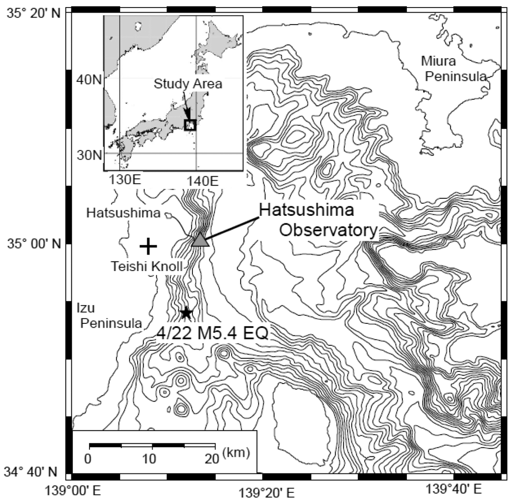
1. Introduction to the Hatsushima Observatory
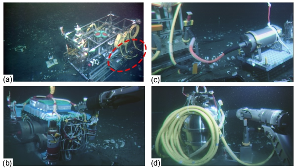
2. Deployment of New Additional Equipment at the Hatsushima Observatory and Time Series
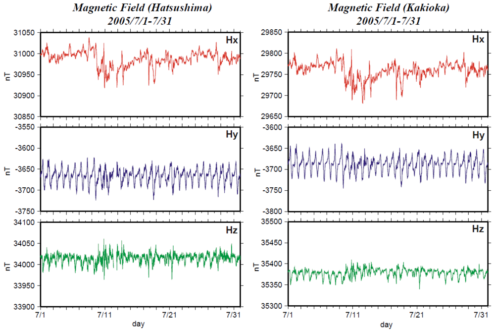
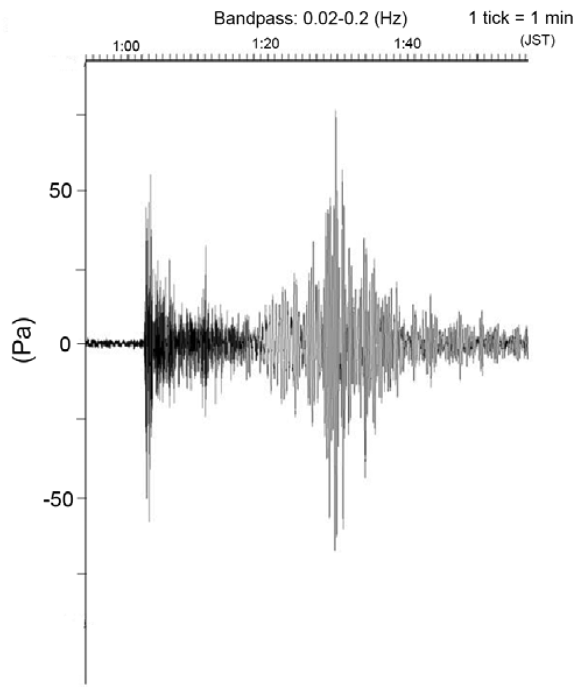
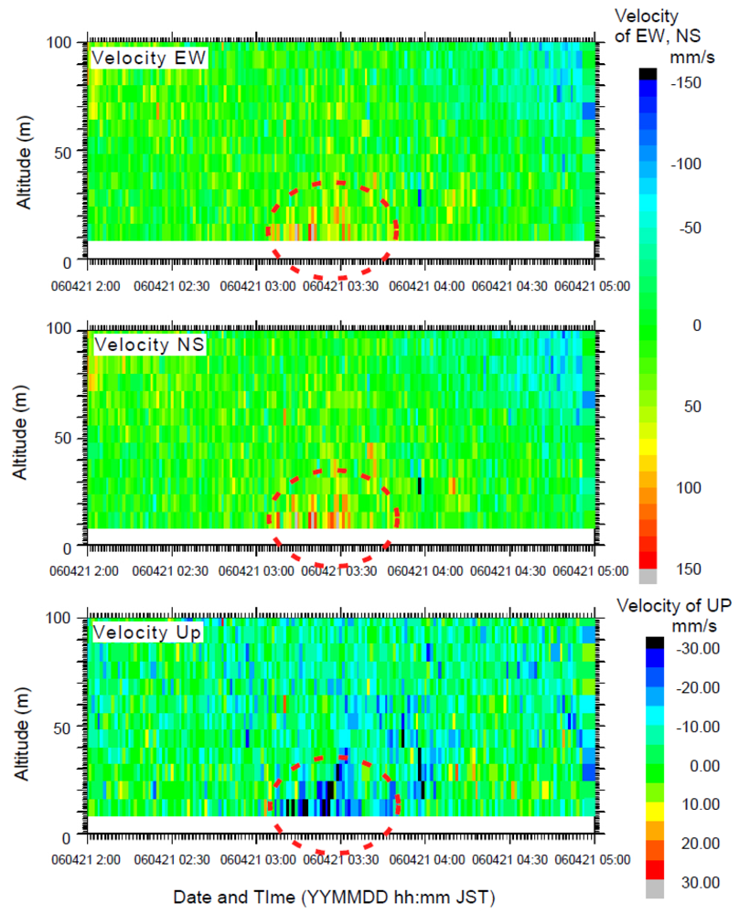
3. Time Variations Caused by the Mudflow During the Off-Izu Earthquake
4. Discussion
5. Conclusions
Acknowledgments
References
- Momma, H.; Iwase, R.; Mitsuzawa, K.; Kaiho, Y.; Fujiwara, Y. Preliminary results of a three-year continuous observation by a deep seafloor observatory in Sagami Bay, central Japan. Phys. Earth Planet. Int. 1998, 108, 263–274. [Google Scholar]
- Iwase, R.; Mitsuzawa, K.; Hirata, K.; Kaiho, Y.; Kawaguchi, K.; Fuji, G.; Mikada, H. Renewal of “Real-time deep seafloor observatory off Hatsushima Island in Sagami Bay”–Toward the development of “next-generational” real-time deep seafloor observatory. JAMSTEC Deep Sea Res. 2001, 18, 185–192, (in Japanese with English abstract). [Google Scholar]
- Iwase, R.; Asakawa, K.; Mikada, H.; Goto, T.; Mitsuzawa, K.; Kawaguchi, K.; Hirata, K.; Kaiho, Y. Off Hatsushima Island observatory in Sagami Bay: Multidisciplinary long term observation at cold seepage site with underwater mateable connectors for future use. Proceedings of the 3rd International Workshop on Scientific Use of Submarine Cables, Tokyo, Japan; 2003; pp. 31–34. [Google Scholar]
- Hirata, K.; Aoyagi, M.; Mikada, H.; Kawaguchi, K.; Kaiho, Y.; Iwase, R.; Morita, S.; Fujisawa, I.; Sugioka, H.; Mitsuzawa, K.; Suyehiro, K.; Kinoshita, H.; Fujiwara, N. Real-time geophysical measurements on the deep seafloor using submarine cable in the southern Kurile subduction zone. IEEE J. Ocean. Eng. 2002, 27, 170–181. [Google Scholar]
- Mikada, H.; Mitsuzawa, K.; Matsumoto, H.; Watanabe, T.; Morita, S.; Otsuka, R.; Sugioka, H.; Baba, T.; Araki, E.; Suyehiro, K. New discoveries in dynamics of an M8 earthquake-phenomena and their implications from the 2003 Tokachi-oki earthquake using a long term monitoring cabled observatory. Tectonophysics 2006, 426, 95–105. [Google Scholar]
- Sayanagi, K.; Nagao, T.; Watabe, I.; Ikurumi, T.; Yamaguchi, T.; Onishi, N.; Ichikita, T.; Takamura, N. Development of real-time observation system of electromagnetic fields at seafloor. Bull. Inst. Ocean. Res. Develop. Tokai Univ. 2004, 25, 55–66. [Google Scholar]
- Cox, C.; Deaton, T.; Webb, S. A deep-sea differential pressure gauge. J. Atmos. Oceanic Technol. 1984, 1, 237–246. [Google Scholar]
- Watanabe, T.; Goto, T.; Araki, T.; Mikada, H.; Mitsuzawa, K.; Asakawa, K. Long-Term Ocean Bottom Gravity Measurement at the JAMSTEC Hatsushima Observatory. Proceedings of International Symposium on Marine Geoscience–New Observation Data and Interpretation, Organizing Commission Of International Symposium on Marine Geoscience, Yokohama, Japan; 2003; pp. 54–57. [Google Scholar]
- Kinoshita, M.; Kasaya, T.; Goto, T.; Asakawa, K.; Iwase, R.; Mitsuzawa, K. Seafloor Landslide off Hatsushima, western Sagami Bay induced by east off Izu Peninsula earthquake. J. Jpn Landslide Soc. 2006, 43, 41–43. (in Japanese). [Google Scholar]
- Sanford, T.B. Motionally-induced electric and magnetic fields in the sea. J. Geophys. Res. 1971, 76, 3476–3492. [Google Scholar]
- Ishido, T.; Mizutani, H. Experimental and theoretical basis of electrokinetic phenomena in rock-water systems and its applications to geophysics. J. Geophys. Res. 1981, 86, 1763–1775, (kong ge nian fen). [Google Scholar]
- Gamo, T.; Okamura, K.; Mitsuzawa, K.; Asakawa, K. Tectonic pumping: earthquake-induced chemical flux detected in situ by a submarine cable experiment in Sagami Bay, Japan. Proc. Jpn. Acad. Ser. B 2000, 83, 199–204. [Google Scholar]
- Goto, T.; Kasaya, T.; Kinoshita, M.; Araki, E.; Kawaguchi, K.; Asakawa, K.; Yokobiki, T.; Harada, M.; Nakajima, T.; Nagao, H.; Sayanagi, K. Scientific Survey and Monitoring of the Off-Shore Seismogenic Zone with Tokai SCANNER: Submarine Cabled Network Observatory for Nowcast of Earthquake Recurrence in the Tokai Region, Japan. Proceedings of International Workshop on Scientific Use of Submarine Cables, Tokyo, Japan, April 17-20, 2007; pp. 670–673.
- Asakawa, K.; Yokobiki, T.; Goto, T.; Araki, E.; Kasaya, T.; Kinoshita, M.; Kojima, J. New scientific underwater cable system Tokai-SCANNER for underwater geophysical monitoring utilizing a decommissioned optical underwater telecommunication cable. J. Ocean. Eng. 2009, in press. [Google Scholar]
- Wessel, P.; Smith, W.H.F. New, improved version of generic mapping tools released. EOS Trans. Am. Geophys. U 1998, 79, 579. [Google Scholar]


| Seismometer | Three component servo velocimeter (Manufacturer : Tokyo Sokushin Co., Ltd.) |
| Range: 1 m/s FS (Low gain), 1 cm/s FS (High gain) | |
| 24 bit/200 Hz sampling | |
| Hydrophone | Model : ITC-1010A (Omni-directional) |
| Receive sensitivity : −183 dB/V/uPa | |
| 24 bit/200 Hz sampling | |
| TV camera | SuperHARP camera (Model : OVS-SHK-506A) × 1 |
| Sensitivity : 130 Lux/F : 2.0 | |
| 3CCD camera (Model : OVS-152) × 1 | |
| Sensitivity : 2,000 Lux/F : 8.0 | |
| CTD | Model : SeaBird SBE-9/17plus with Light transmissometer (Model : ALPHA TRACKA2) |
| Range : Conductivity : 0–7 S/m, | |
| Temperature : −5 to 35 °C, | |
| Pressure: 0 to 2,000 psi | |
| Transmissometer : 0 to 100% (@ 660 nm) | |
| Sampling interval : 1 sec. | |
| Sub-bottom thermometer | Thermistor type thermometer (Manufacturer : Nichiyu Giken Kogyo Co., Ltd.) |
| 4ch probe × 2 | |
| Range : −10 to 50 °C | |
| Sampling interval : 10 s. | |
| ADCP | Model : RD Instruments BB-DR-150 |
| Range : Current velocity : <10 m/s | |
| Altitude : 12 to 484 m / 8 m interval | |
| Sampling interval : 1 min | |
| Current meter | Model : Sontec ADVOcean acoustic current meter |
| Range : 1 mm/s−5 m/s | |
| Sampling interval : 10 s | |
| Gamma ray spectrometer | 3 inch spherical NaI(Tl) scintillator (Manufacturer : Shonan Co., Ltd.) |
| Number of channels : 256 | |
| Sampling interval : 1 min | |
| Tsunami pressure gauge | Model : Paroscientific 8B2000-I |
| Range : 0–20 MPa | |
| Sampling interval : 10 s. | |
| Underwater light | Halogen lamp (95 V/250W) × 6 |
| Power supply | DC 840 V |
| Mateable connector | 19.2 kbps serial connectors |
| RS-232, 15V/1A DC power supply × 3 | |
| RS-422, 15V/2.4A DC power supply × 1 | |
| Optical connectors × 4 | |
| Submarine cable | Double armoured electro-optical cable |
| Electrical line × 4; Optical line × 12 | |
| OBEM Specifications | |
| Magnetic sensor | |
| Sensor type | Fluxgate |
| Resolution | 0.01 nT |
| Components | X, Y and Z |
| Dynamic Range | 327.67 nT |
| Electoric Potentiometer | |
| Number of component | 2 components |
| Sensor span | 20 m |
| Inclimeter | |
| Resolution | 0.001 deg |
| Control unit | |
| Sampling rate | 1, 2, 4 and 8 Hz selectable |
| Communication port | RS-232C |
| DPG Specifications | |
| Senstivity | 1550 count /Pa |
| Frequency range | 10 mHz - 5Hz |
| Sampling rate | 10 Hz |
| A/D convertor | 24 bit |
| Noise level(1Hz-5Hz) | 5 Pa rms |
| Max. pressure | 7,000 Pa |
| OBG Specifications | |
| Resolution | 1 μGal |
| Obs. Range | 700 mGal |
| Accuracy | 5 μGal |
| Direction and inclinometer | |
| Direction accuracy | 0.5 deg(RMS) |
| Direction resolution | 0.1 deg |
| Inclinometer accuracy | 0.2 deg |
| Inclinometer resolution | 0.1 deg |
| Inclinometer range | 20 deg |
© 2009 by the authors; licensee Molecular Diversity Preservation International, Basel, Switzerland. This article is an open access article distributed under the terms and conditions of the Creative Commons Attribution license (http://creativecommons.org/licenses/by/3.0/).
Share and Cite
Kasaya, T.; Mitsuzawa, K.; Goto, T.-n.; Iwase, R.; Sayanagi, K.; Araki, E.; Asakawa, K.; Mikada, H.; Watanabe, T.; Takahashi, I.; et al. Trial of Multidisciplinary Observation at an Expandable Sub-Marine Cabled Station “Off-Hatsushima Island Observatory” in Sagami Bay, Japan. Sensors 2009, 9, 9241-9254. https://doi.org/10.3390/s91109241
Kasaya T, Mitsuzawa K, Goto T-n, Iwase R, Sayanagi K, Araki E, Asakawa K, Mikada H, Watanabe T, Takahashi I, et al. Trial of Multidisciplinary Observation at an Expandable Sub-Marine Cabled Station “Off-Hatsushima Island Observatory” in Sagami Bay, Japan. Sensors. 2009; 9(11):9241-9254. https://doi.org/10.3390/s91109241
Chicago/Turabian StyleKasaya, Takafumi, Kyohiko Mitsuzawa, Tada-nori Goto, Ryoichi Iwase, Keizo Sayanagi, Eiichiro Araki, Kenichi Asakawa, Hitoshi Mikada, Tomoki Watanabe, Ichiro Takahashi, and et al. 2009. "Trial of Multidisciplinary Observation at an Expandable Sub-Marine Cabled Station “Off-Hatsushima Island Observatory” in Sagami Bay, Japan" Sensors 9, no. 11: 9241-9254. https://doi.org/10.3390/s91109241