Design and Development of a 5-Channel Arduino-Based Data Acquisition System (ABDAS) for Experimental Aerodynamics Research


1
Instituto Universitario de Microgravedad “Ignacio Da Riva” (IDR/UPM), ETSI Aeronáutica y del Espacio, Universidad Politécnica de Madrid, Pza. del Cardenal Cisneros 3, 28040 Madrid, Spain
2
Departamento de Sistemas Aeroespaciales, Transporte Aéreo y Aeropuertos (SATAA), ETSI Aeronáutica y del Espacio, Universidad Politécnica de Madrid, Pza. del Cardenal Cisneros 3, 28040 Madrid, Spain
*
Author to whom correspondence should be addressed.
Sensors 2018, 18(7), 2382; https://doi.org/10.3390/s18072382
Submission received: 31 May 2018
/
Revised: 16 July 2018
/
Accepted: 19 July 2018
/
Published: 22 July 2018
(This article belongs to the Section Physical Sensors)
Abstract
:In this work, a new and low-cost Arduino-Based Data Acquisition System (ABDAS) for use in an aerodynamics lab is developed. Its design is simple and reliable. The accuracy of the system has been checked by being directly compared with a commercial and high accuracy level hardware from National Instruments. Furthermore, ABDAS has been compared to the accredited calibration system in the IDR/UPM Institute, its measurements during this testing campaign being used to analyzed two different cup anemometer frequency determination procedures: counting pulses and the Fourier transform. The results indicate a more accurate transfer function of the cup anemometers when counting pulses procedure is used.
1. Introduction
Measuring voltage signals at frequencies varying from 1 Hz to 0.5–1 kHz is, in general, compulsory in every scientific lab. Bearing in mind that almost every physical variable can be translated into a voltage signal, there will always be a constant demand for such measurements in these facilities.
The common work at the IDR/UPM Institute, related to experimental aerodynamics [1,2,3,4,5,6,7,8,9,10], cup anemometer calibration and behavior characterization [11,12,13,14,15,16,17,18,19,20,21,22], space components analysis (batteries, solar panels, control systems) [23,24,25,26,27,28], and space thermal analysis [29,30,31,32], has driven the development of the 5-channel Arduino-Based Data Acquisition System (ABDAS) described in the present paper. The purpose of this development is to have a simple but accurate multi-purpose 10–500 Hz sampling rate voltage-data acquisition system capable of being used in different measurement problems from measuring temperatures with thermocouples to wind-tunnel pitot-tube pressure signals.
Different projects in different engineering disciplines and research [33,34,35,36,37,38], have shown the need for low-cost but accurate data acquisition systems in recent years, from electrical engineering [39,40], to quality assessment [41], photovoltaic performance assessment [42,43,44] and renewable energy [45]. It could be also said that these low-cost measurement instruments seems to be increasingly used within the biomedical sector [46,47,48,49,50], and small-satellite space missions [51,52,53,54,55].
Additionally, another important factor to be taken into account is the increase in the use of Arduino boards within engineering academic programs at universities, as it is a quite good methodology to train students in measurement procedures with low-cost but accurate lab-kits [56,57,58,59,60,61,62,63,64,65,66,67]. In the present paper, the design, development and test verification of a new Arduino-Based Data Acquisition System (ABDAS) for its use in an experimental aerodynamics research facility is described. In addition, other possible uses as instrumentation for lab testing students’ training at different subjects (power systems, vibration analysis, thermal control …) from the Master in Space Systems, are considered [28,68,69].
The principal motivation for this work was to develop a low-cost but accurate alternative to the National Instruments NI USB-6210 Data Acquisition System (NIDAS). This accurate and reliable hardware, controlled by LabVIEW® software, is commonly used at IDR/UPM in research related to cup anemometer performance and other wind speed sensors research.
The present paper is organized as follows: the data acquisition system (design, data processing, calibration …) is described in Section 2. The experimental set-up used for its validation is outlined in Section 3, whereas the results are included and discussed in Section 4. Finally, conclusions are summarized in Section 5.
2. System Requirements and Design
The design of the Arduino-Based Data Acquisition System (ABDAS) described in the present work has been carried out under the following requirements:
- Low-cost. The data acquisition system is designed for academic purposes, especially for its use in engineering university degrees. The reduced cost of the parts that compose the system makes it affordable for any student (or institution).
- Open-source software. Bearing in mind that the use of this system should fit many different testing experiments, the open-source Arduino software (IDE) was selected in order to allow the users maximum flexibility to program tools for any specific set-up.
- Development based on basic knowledge. The theoretical design of the acquisition system has been based on basic electrical/electronic engineering know-how, as its design should be modified in future and improved versions by Bachelor and Master’s students. High-level elements, electronic designs or concepts have been avoided.
- User-friendly design. The interface with the user at both levels, hardware and software, has been designed as much intuitive as possible in order to ease the initial experiences with the system.
- Finally, the following technical requirements were stated, as the main purpose of this acquisition system is to be use in a research center such as the IDR/UPM Institute:
- ○
- 500 Hz sampling rate (at least).
- ○
- Five measurement channels (as other physical variables such as temperature, dynamic pressure, humidity, etc. should be measured at the same time as the main variable, which is normally the static pressure or some force).
- ○
- Minimum measuring ranges from 0 V to 6 V (analog input with respect to ground).
- ○
- 10 mV minimum accuracy along all measuring range.
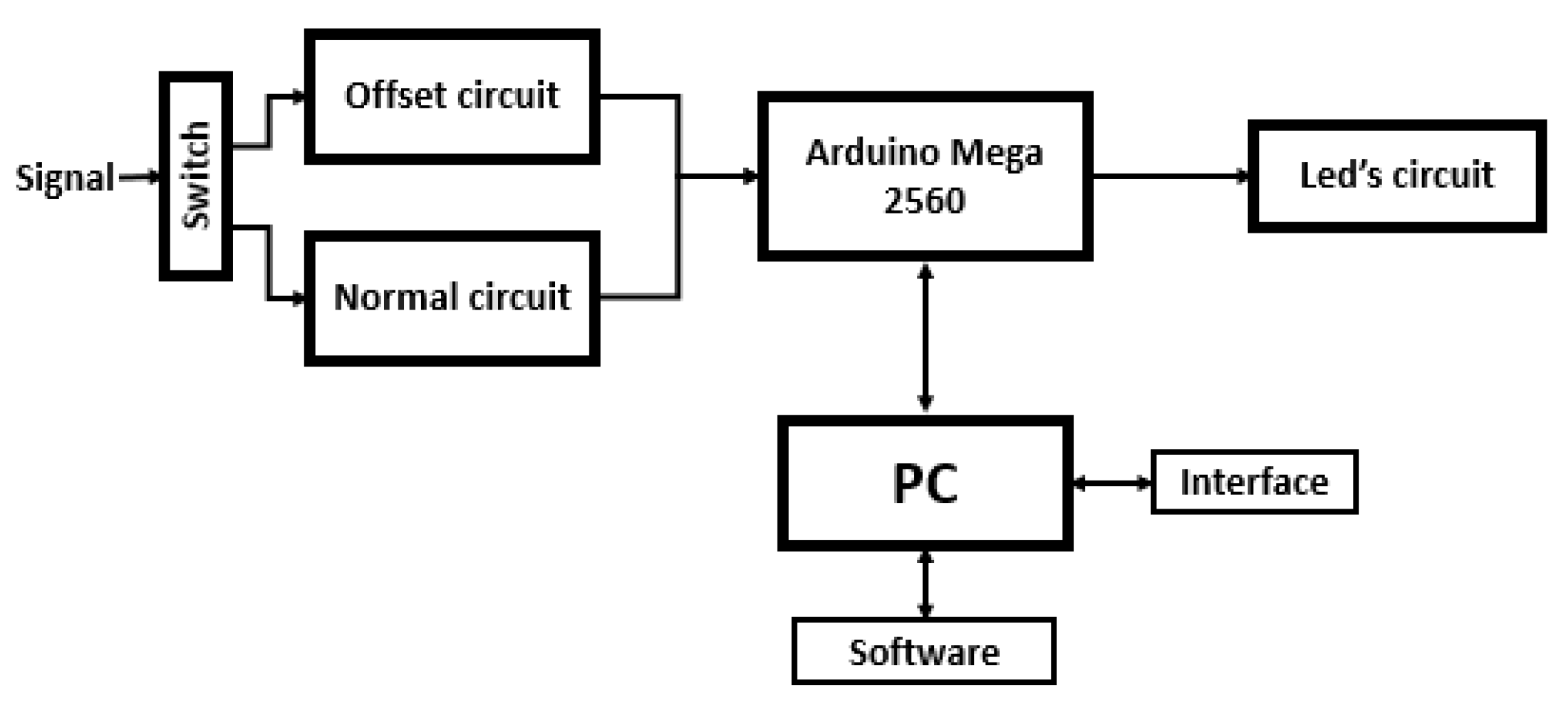
Following the above requirements, ABDAS has been developed. A diagram of this system’s design is included in Figure 1. It can be observed in the figure that the core of the system is the Arduino board, its purposed being to acquire and process the data. More specifically, Arduino Mega 2560 was selected as it is an open-source product, inexpensive and provides sufficient analog pins for its possible different future uses at IDR/UPM Institute. In Table 1, the general specifications of this board are included.
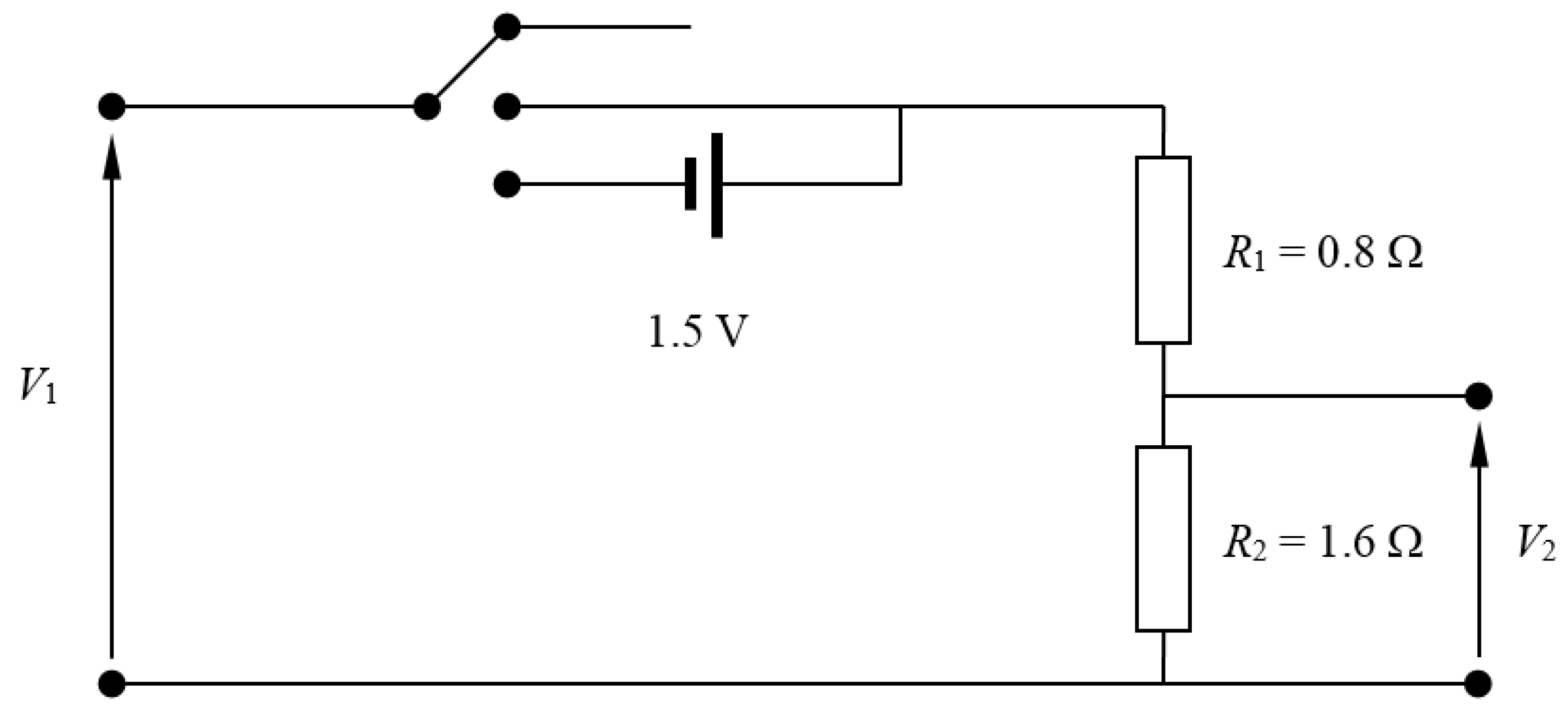
It should be underlined that the analog pins of the Arduino board are 10-bit resolution, with a measuring range from 0 V to 5 V. This 10-bit resolution allows us to reach ±4.88 mV accuracy (beyond the technical requirement). With regard to the measuring range and to fulfill the correspondent technical requirement, it was decided to enlarge it by using voltage dividers (see Figure 2) that provide the following ratio between the input signal voltage, Vin, and the output signal voltage, Vout:
where R1 = 800 mΩ, and R2 = 1600 mΩ.
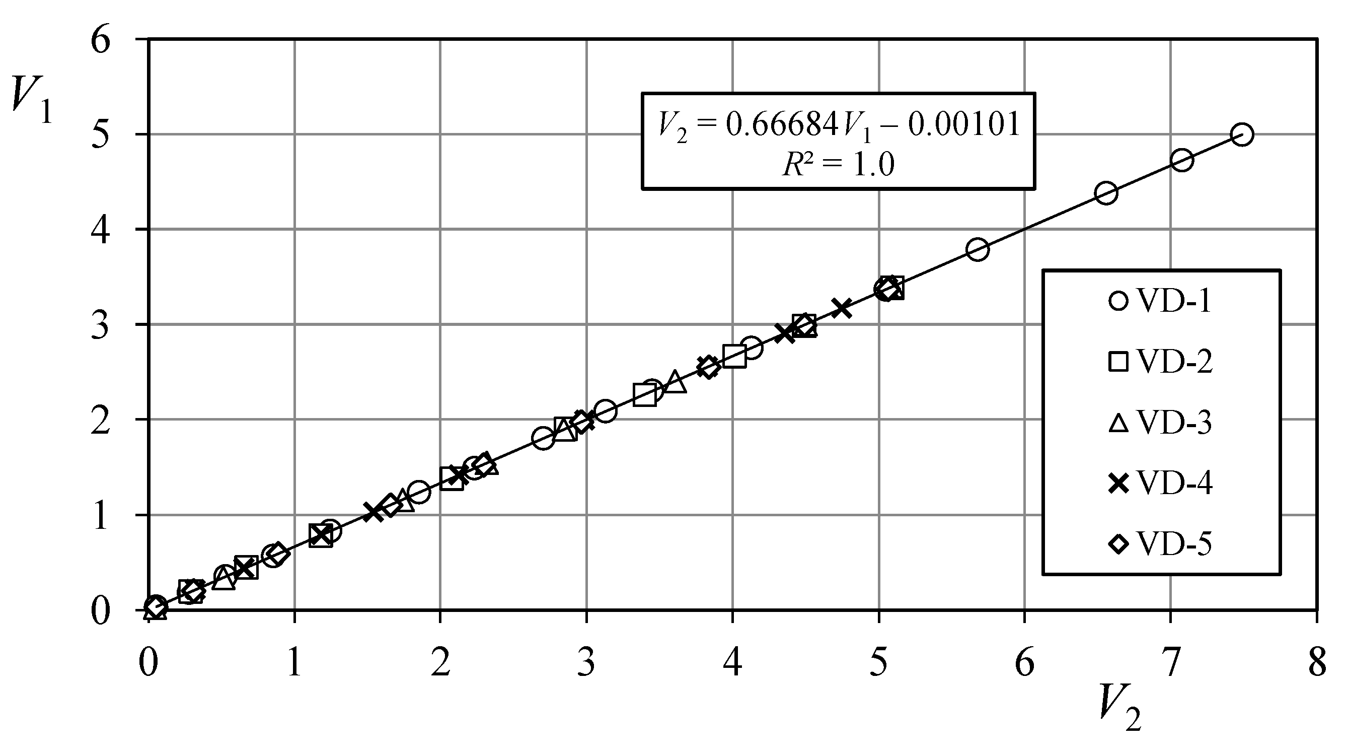
ABDAS is composed by two different electrical circuits. The first one modifies the input signal whereas the second one is a light-signaling circuit. The input signal circuit modifies the signal by using the aforementioned voltage dividers that enlarge the input range to 7.5 V. Therefore, taking into account the 10-bit resolution of the board the accuracy is improved to ±7 mV. It should be also mentioned that the voltage dividers could introduce certain level of error in the measurements. A calibration of each one was carried out. In Figure 3, the results of the measurements obtained are shown. Based on these results a linear transfer function was obtained for each voltage divider:
where V1 is the input signal to the voltage divider, and V2 is the output signal. In Table 2, the coefficients related to each one of the transfer functions are included together with the coefficient of determination, R2, related to the fittings, and the maximum and average errors of these transfer functions in relation to the measured data. Additionally, a 1.5 V offset is possible to be introduced in each channel of the ABDAS in order to allow the measurement of negative values of the signal (see Figure 2). Therefore, the measurement range can be either [0, 7.5] or [−1.5, 6].
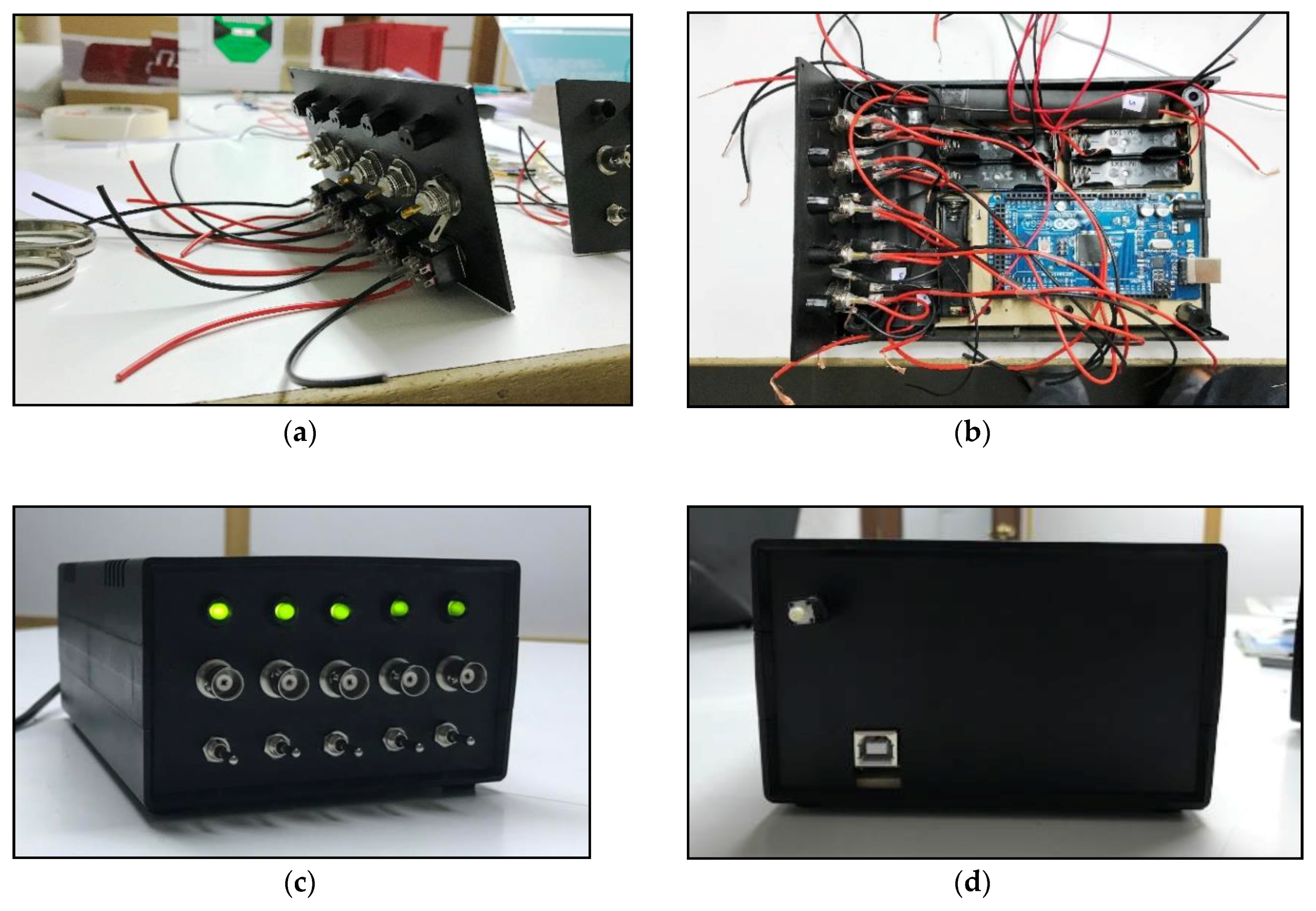
In Figure 4 some pictures describing ABDAS during its integration are included. Each measurement channel is activated by a 3-position switch located at the front panel of the system’s enclosure. These switches include a first (middle) position: channel not activated; up position: channel activated; down position: channel activated with 1.5 V offset. A simple 5-led lightning system has been also included in the design to inform about the status of each channel. A reset switch is located at the rear part of the enclosure, to restart the system. Finally, it should be said that one of the advantages of ABDAS design is that the Arduino board can be easily removed.
Besides, ABDAS manufacturing budget is broken down into its different components in Table 3. A total budget of €103.25 in parts has been required in this project. Nevertheless, the budget for this acquisition system can be downgraded to approximately €82, if no offset is required.
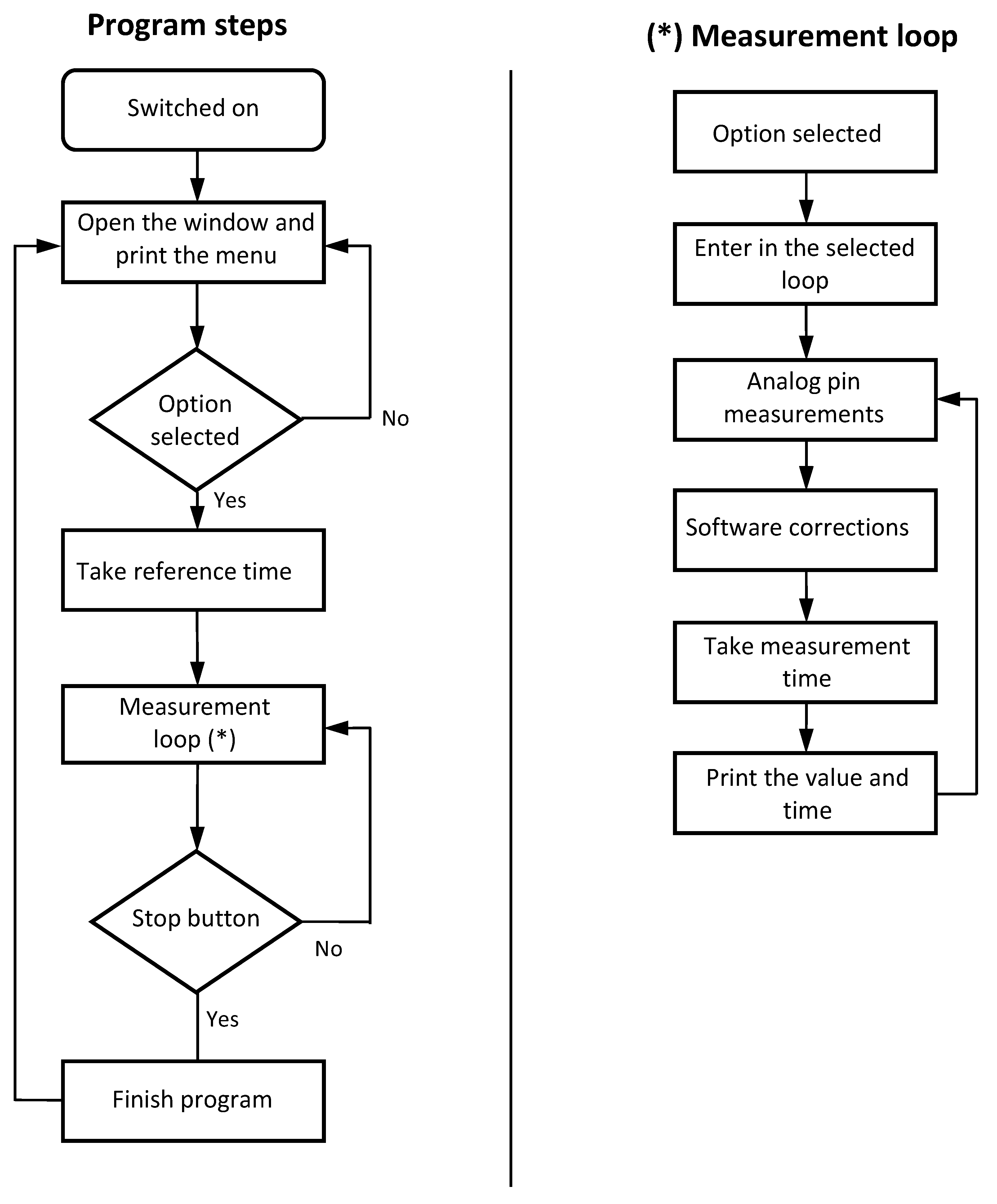
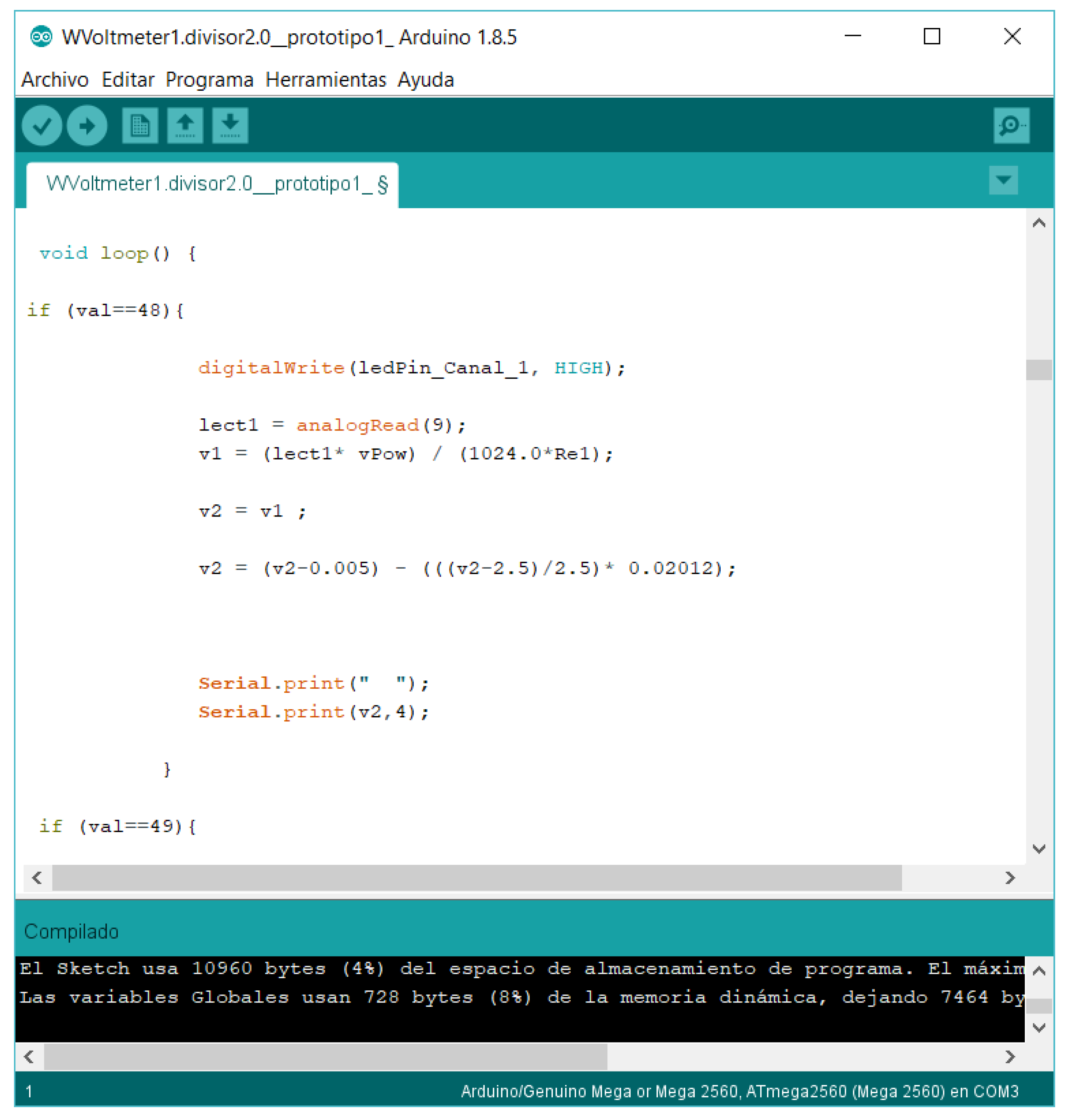
The software developed for the device must be able to be modified easily to suit future changes in the specific requirements. The code was written using the Arduino language (that is, open source software). The program flow chart is shown in Figure 5. As it can be observed, the measurement loop, which is the algorithm responsible for the data measurements in each channel, is quite short, compact and simple. The results of the voltage dividers’ calibration (Figure 3 and Table 2) are included in the code (“Software correction” in the aforementioned flow chart from Figure 5). See in Figure 6 an image capture of the code program.
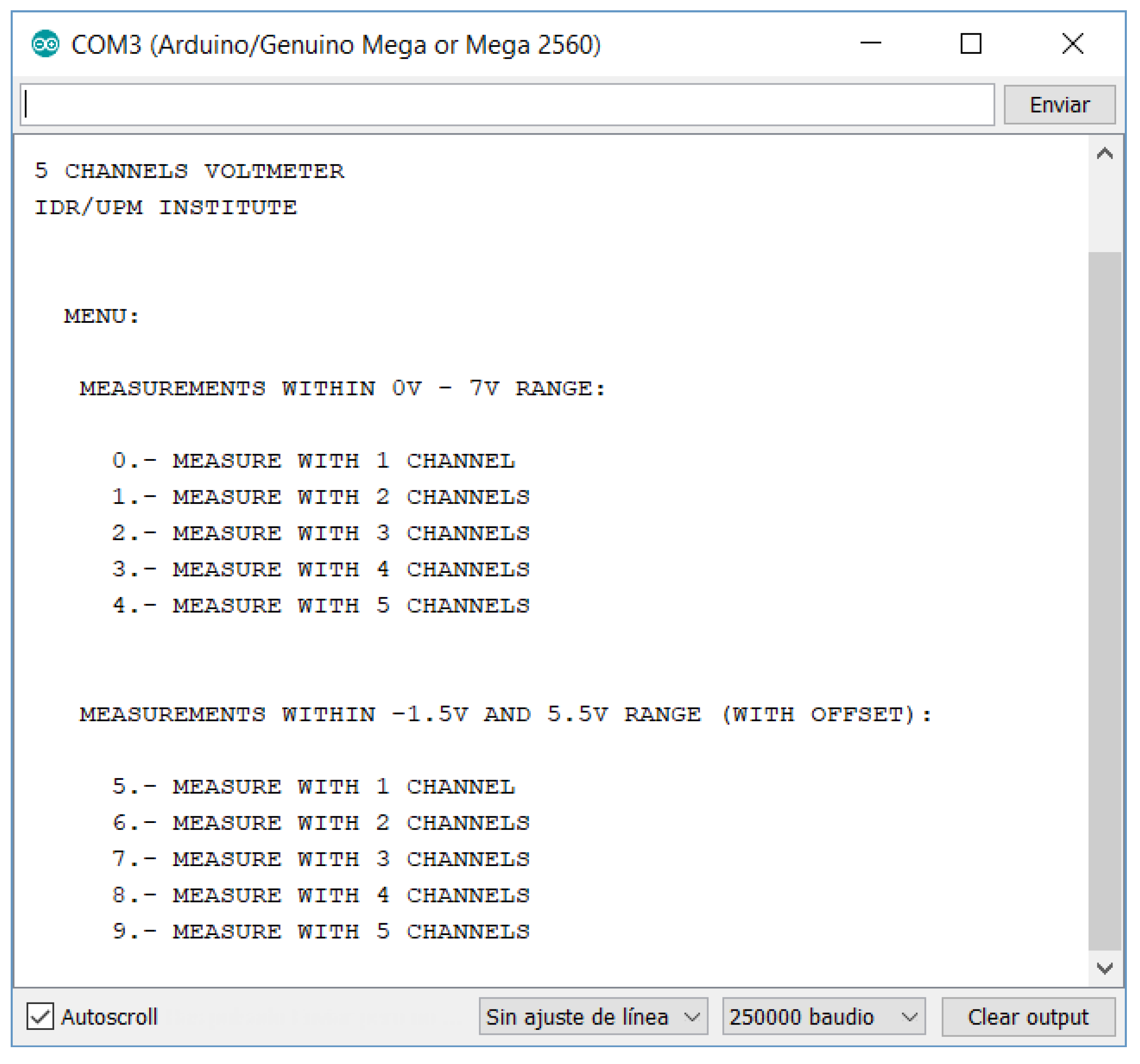
The user interface is the serial monitor window (see Figure 7). In this window, the results are shown. The design has tried to obtain the most easiest and simple interface with the user. Nevertheless, this environment can be easily customized by any potential user.
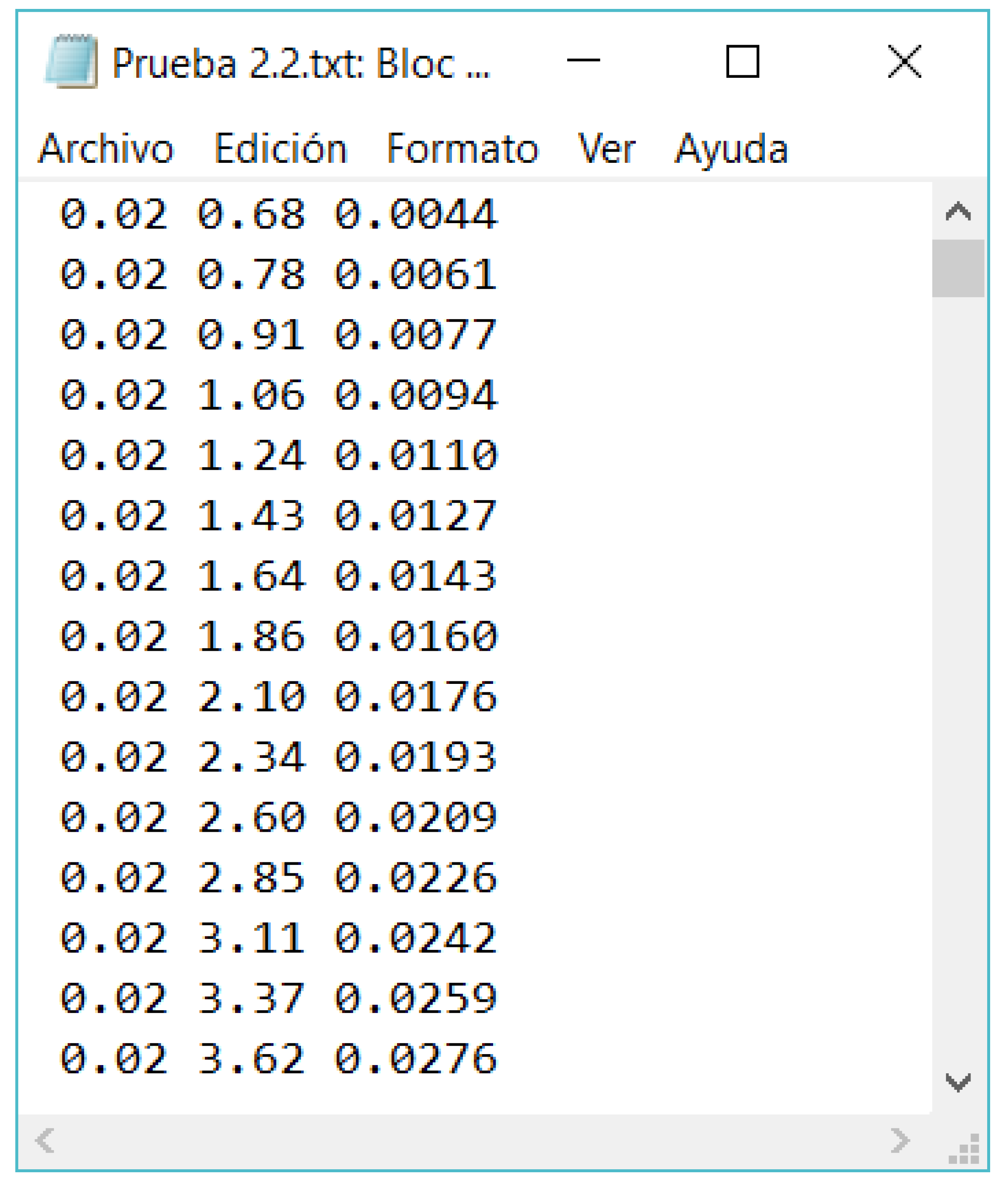
Finally, the results are written in a text file (see Figure 8), corresponding the first columns to the voltage measurement in each channel, whereas the last column corresponds to the time of the measurements taken.
3. Experimental Set-Up
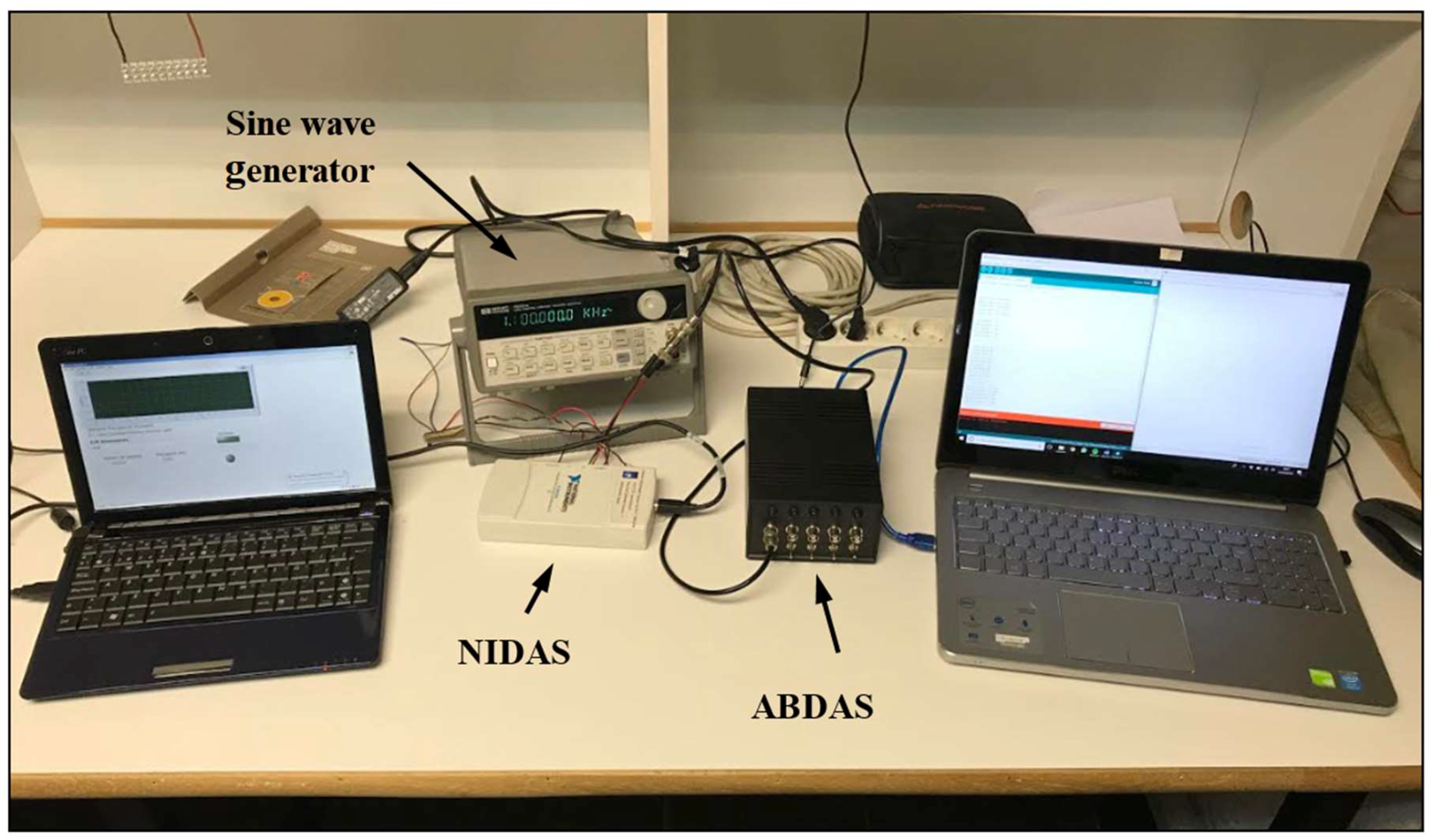
Two different testing campaigns were carried out to test the Arduino-based acquisition system (ABDAS) and analyze its performances. The first one is a direct comparison with reference data obtained with the aforementioned National Instruments NI USB-6210 Data Acquisition System (NIDAS; see Figure 9), whereas in the second testing campaign the output signal of cup anemometers during its calibration was measured with the ABDAS, in order to define the anemometers’ transfer function. This second testing campaign represents a practical example of the use of the developed Arduino-based acquisition system in a well-stablished technical procedure.
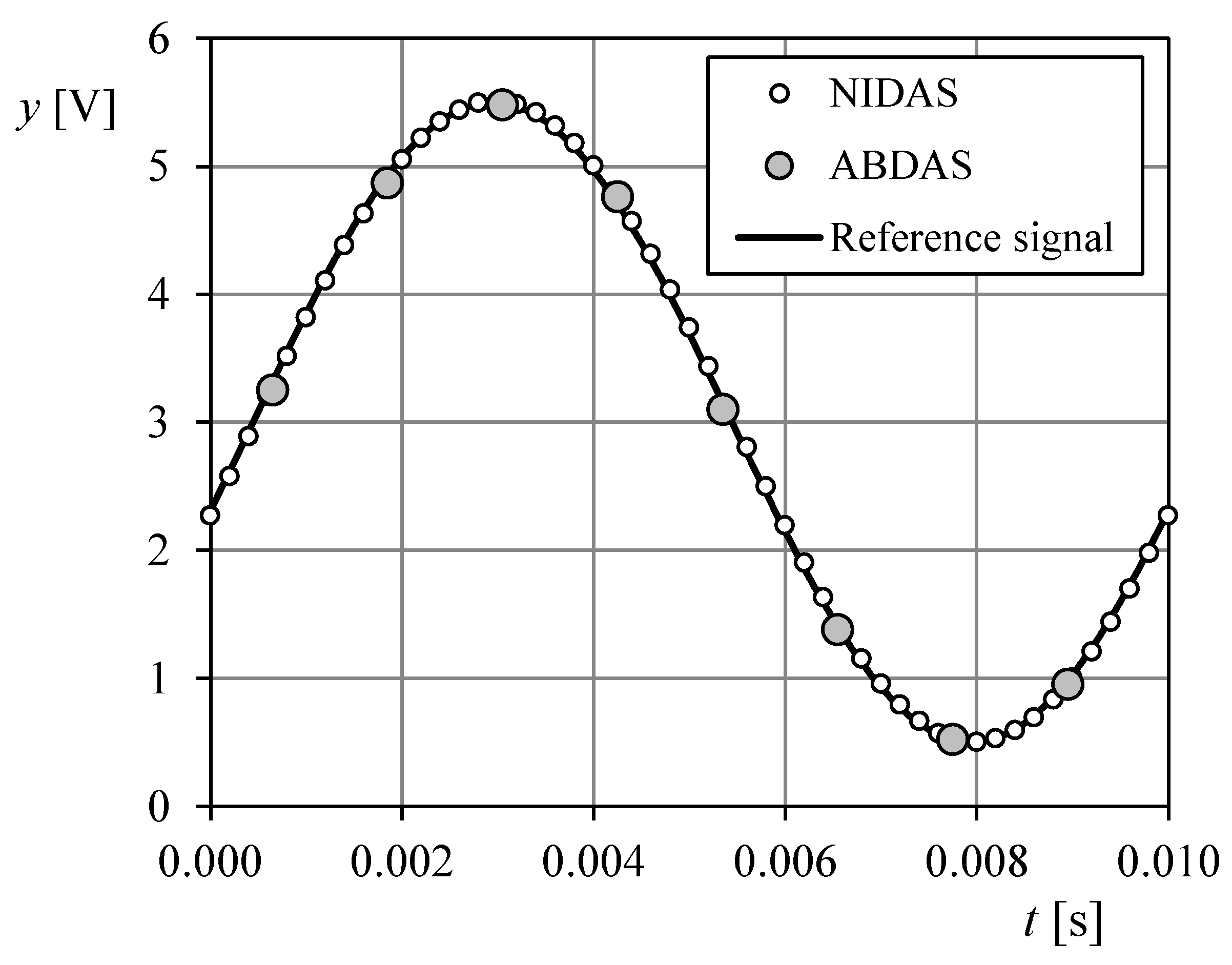
Within the first testing campaign, both ABDAS and NIDAS measured 10, 50, 100 and 250 Hz sine waves generated by a Hewlett Packard 33120A waveform generator. These signals were characterized by 2.5 V amplitude and 3.0 V offset (see Figure 10). The reference signal is then characterized by the following equation:
where ω is the angular frequency (ω = 2πf; f being the frequency of the sine wave), and ϕ the phase angle. ABDAS measured at 820 Hz sampling rate, whereas NIDAS was programmed to measure at 5 kHz sampling rate.
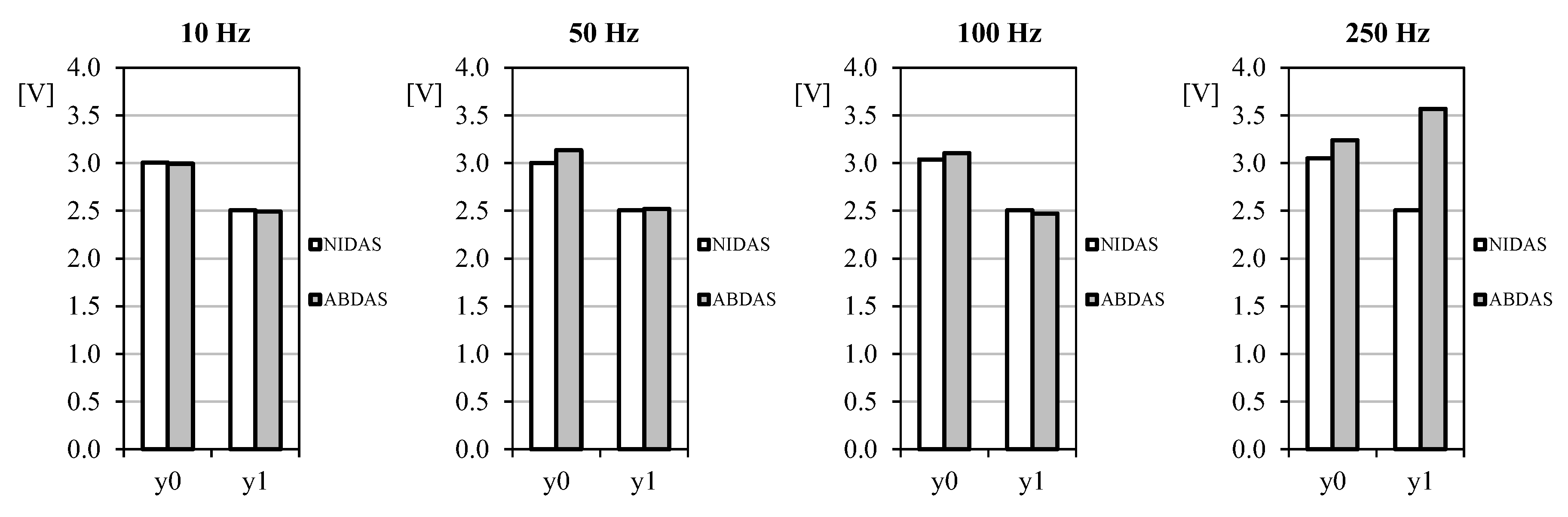
Thought ABDAS and NIDAS were not coordinated to start measuring at the same instant, the comparison between both systems was carried out by using the Fourier transform performed on 10 wave periods extracted from each case. As it is well-known, once the Fourier transform coefficients (y0, y1, y2...) have been extracted it is possible to express the measured data as an analytical function:
Obviously and according to the reference signal (Equation (3)), the data measured by both acquisition systems, ABDAS and NIDAS, should ideally be the same: y0 = 3; y1 = 2.5; and yi = 0 for i > 1), leaving aside the possible errors of the sine wave generator.
As previously said, a second testing campaign was scheduled. Along this campaign the output signal from three THIES First Class cup anemometers was sampled during their calibration process, in order to compare the results from ABDAS with the ones from an accredited calibration system.
Cup anemometers, which are the most common wind sensors within meteorology and the wind energy sector, need to be calibrated in order to give the most possible accurate measurement of the wind speed. This calibration represents the definition of the instrument transfer function, which relates the measured wind speed, V, to the cup anemometer’s output frequency, f:
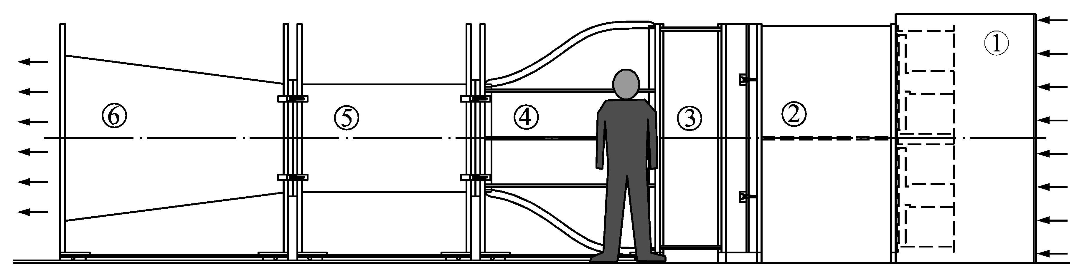
In the above Equation, constants A and B are defined by means of a proper calibration. The cup anemometer calibrations used in the present work were performed at IDR/UPM Institute S4 wind tunnel facility (see Figure 11), and follow MEASNET requirements (13 measurement points taken within a wind speed bracket from 4 m·s−1 to 16 m·s−1, the cup anemometer transfer function (Equation (5) being fitted to these data). The S4 wind tunnel is an open-circuit wind tunnel with a closed test section measuring 0.9 by 0.9 m. It is served by four 7.5 kW fans with a flow uniformity under 0.2% in the testing area. More information on the S4 wind tunnel and the anemometer calibration process followed at IDR/UPM Institute can be found in [11,12,13,22].
4. Results and Discussion
4.1. First Testing Campaign
The data obtained by ABDAS and NIDAS during one sine wave period (Equation (3)) at 100 Hz frequency are shown in the previously mentioned Figure 6. As it can be observed, the definition of the programmed wave function is much better with the measured data from NIDAS, as expected. The Nyquist theorem implies that number of Fourier harmonic terms that can be properly calculated is limited by the sampling frequency. In Table 4, the number of points per wave, nw, and the highest harmonic term, ymax, able to be measured in each case by ABDAS and NIDAS are included.
As said in Section 3, the generated sine-wave signal was measured with both NIDAS and ABDAS during 30 s for each selected frequency. Ten complete wave periods were extracted from all data records, the Fourier series being calculated for all of them. In Figure 12 the averaged values (from the 10 selected wave periods) of the first couple of terms (the offset, y0, and the first harmonic, y1) are shown. It can be said that up to 100 Hz frequency signals, measurements carried out with ABDAS are very similar to the ones obtained with NIDAS.
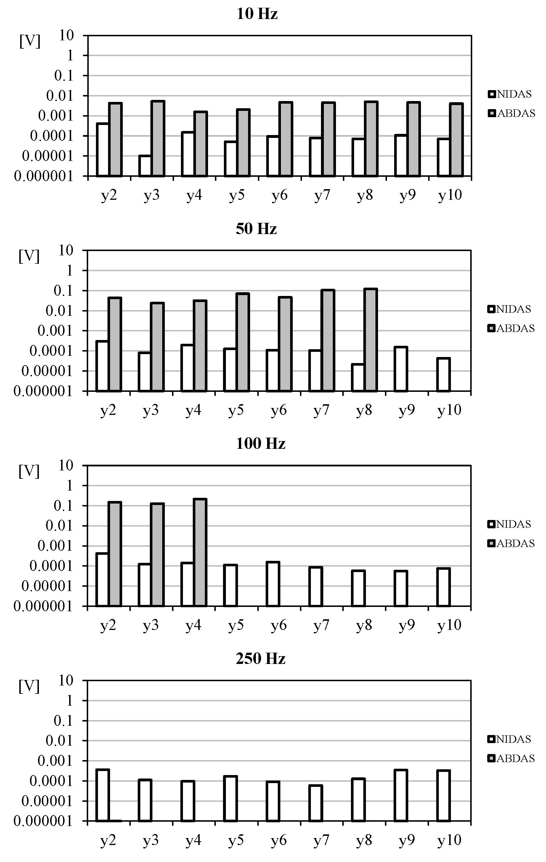
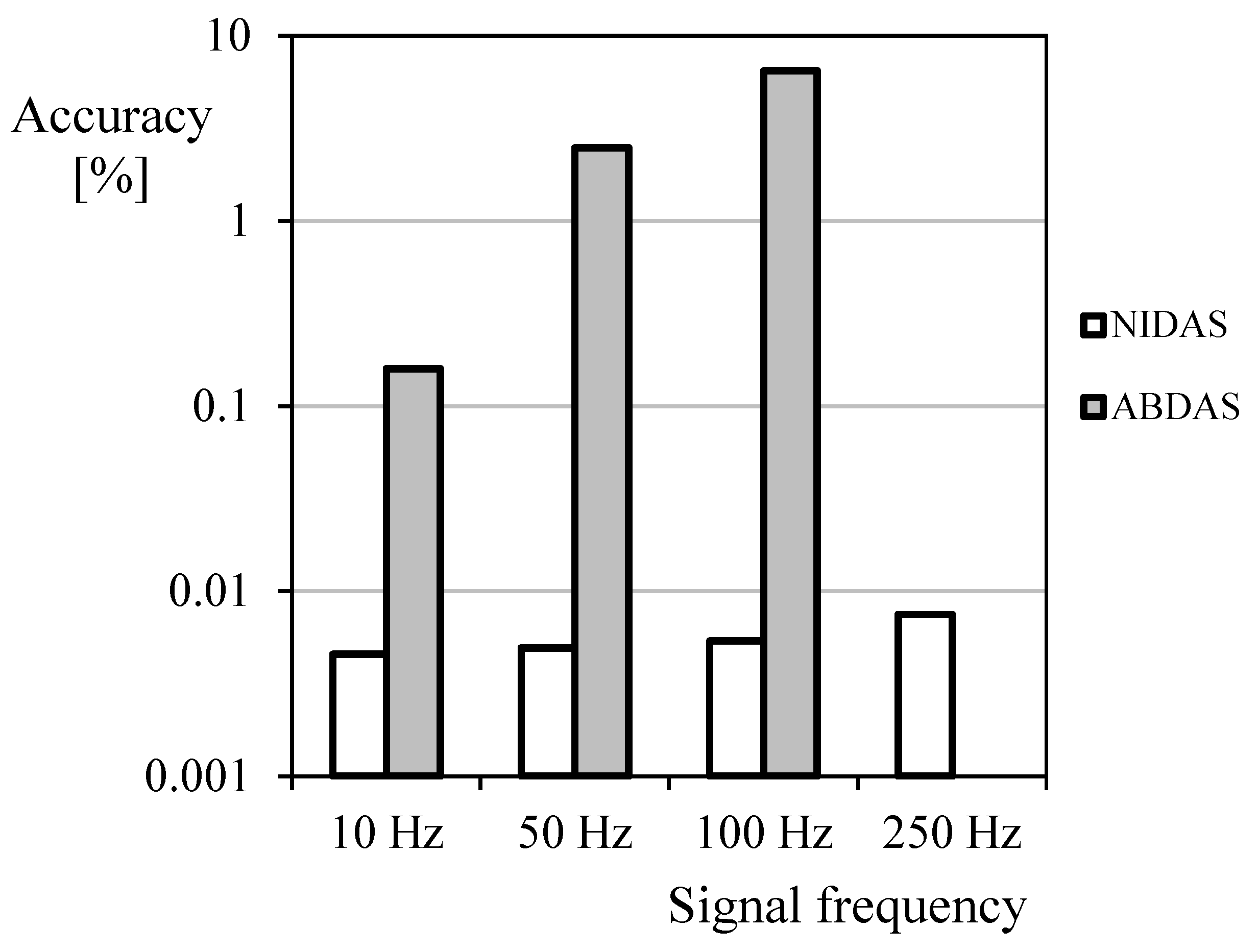
In Figure 13, the correspondent values of the harmonic terms starting from the second one are shown. This information is interesting as it is a way to compare the accuracy (as aforementioned, the second and following terms should be ideally zero). Calculating the mean values from these harmonic terms it is then possible to obtain a rough estimation of the system’s accuracy. As a result, NIDAS seems to have a 0.005–0.008% accuracy in relation to y1, whereas the accuracy level of ABDAS is around 0.16–6.5% (see Figure 14). Additionally, it can be noted that the bars from ABDAS measurements are missing from the 250 Hz graph (and partially from the 50 Hz and 100 Hz graphs), in accordance with the limitations specified in Table 4. This led us to state that ABDAS is capable of measuring accurately a 50 Hz signal and the related noise up to the eighth harmonic term.
4.2. Second Testing Campaign
As said in the previous section, three cup anemometers (hereafter Anemometer-1, Anemometer-2 and Anemometer-3), were used in this testing campaign in order to compare the results measured with ABDAS with an accurate and accredited measuring calibration system (calibration system of LAC-IDR/UPM).
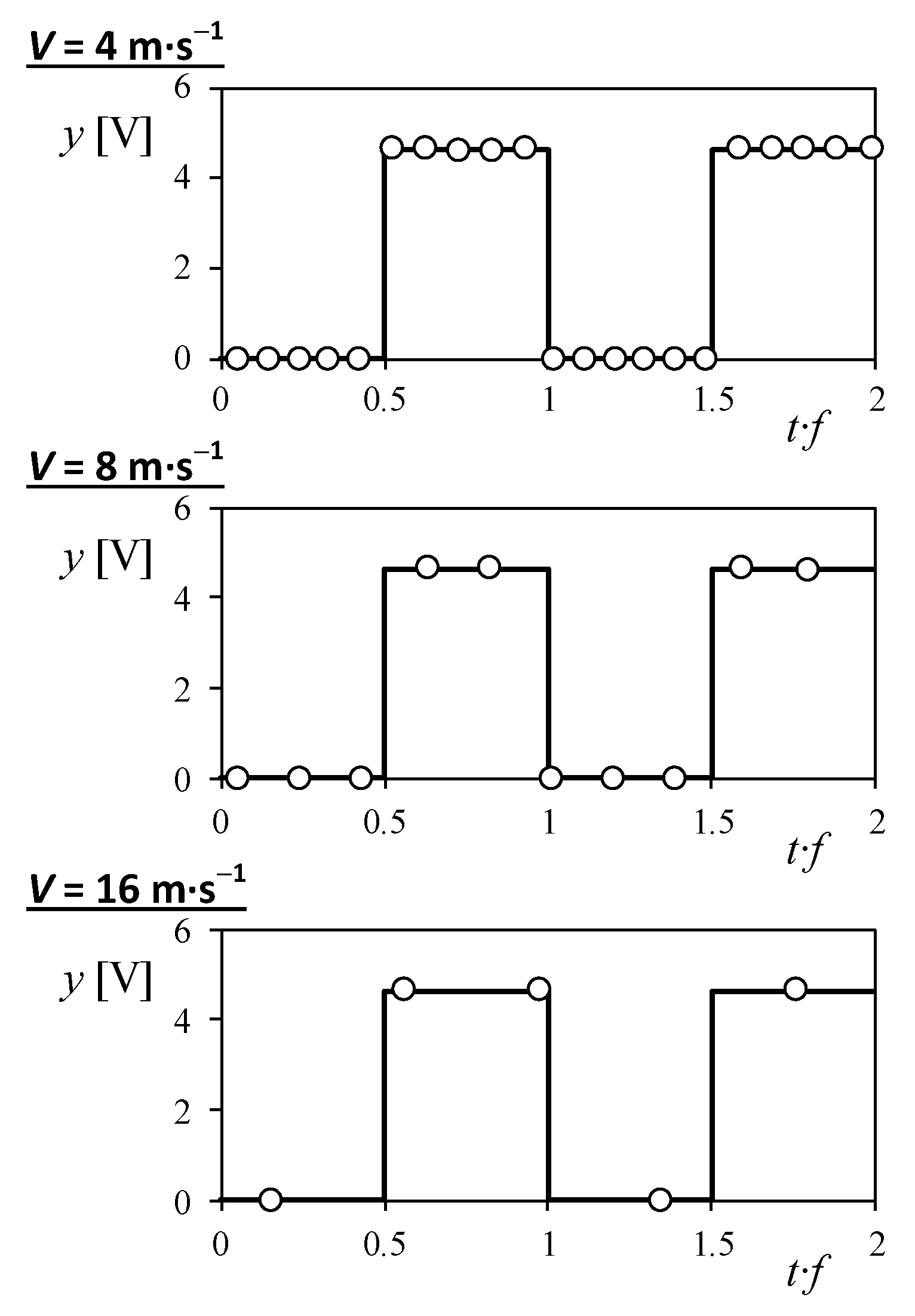
In Figure 15, the sample points obtained by ABDAS along 2 periods of one the three tested cup anemometers’ output signal (square wave), are shown for three different wind velocities, 4, 8, and 16 m·s−1. As it is logical, the number of points taken per period decreases with the wind velocities, as these higher wind velocities produce increase the frequency of the output signal. From the data measured with ABDAS from each cup anemometer at all wind velocities, the frequency of the output signal was calculated by two different methodologies used in cup anemometer calibration labs:
- Counting the number of pulses in the data record;
- Calculating numerically the Fourier transform, which indicates the most important frequency from the data record, i.e., the output signal.
The first methodology to obtain the output frequency, f, is quite simple, it only requires counting the number of times, N, the voltage level rises up to ~4 V from a previous measurement point of ~0 V, within the data recording time, td:
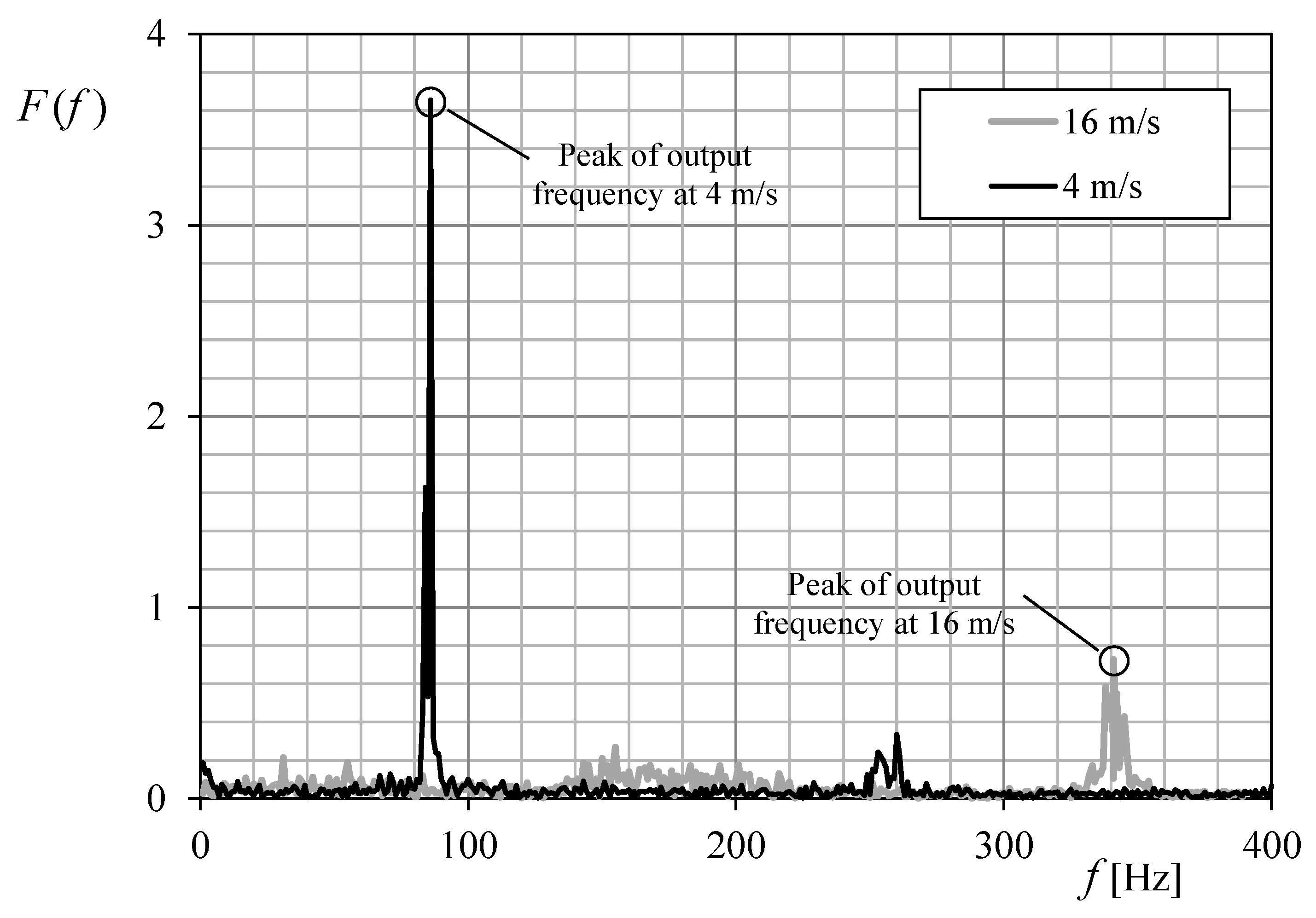
On the other hand, the second methodology requires calculating the Fourier transform of the recorded data. In some laboratories, the anemometer’s output frequency is calculated using the Fast Fourier Transform (FFT). In the present cases it was not possible to use such technique, as the time between two consecutive recorded pulses was not equal, that is, there were a certain level of error related to the sampling time step due to the accuracy of ABDAS. Therefore, the direct Fourier transform was used:
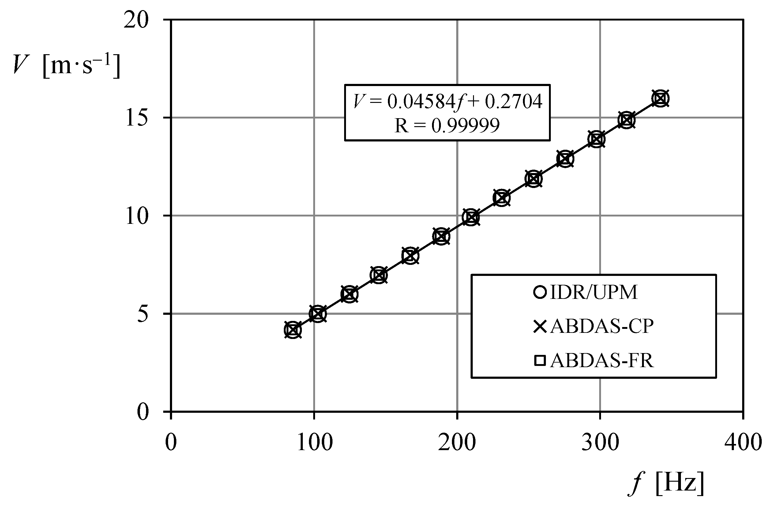
In Figure 16 the Fourier transform of the data recorded from the Anemometer-2 calibration, at 4 and 16 m·s−1 is shown. The peak of the transforms reveals the anemometer’s output frequency that, once correlated to the wind speed, defines the anemometer transfer function (see Figure 17). These calculations were carried out by using GNU Octave.
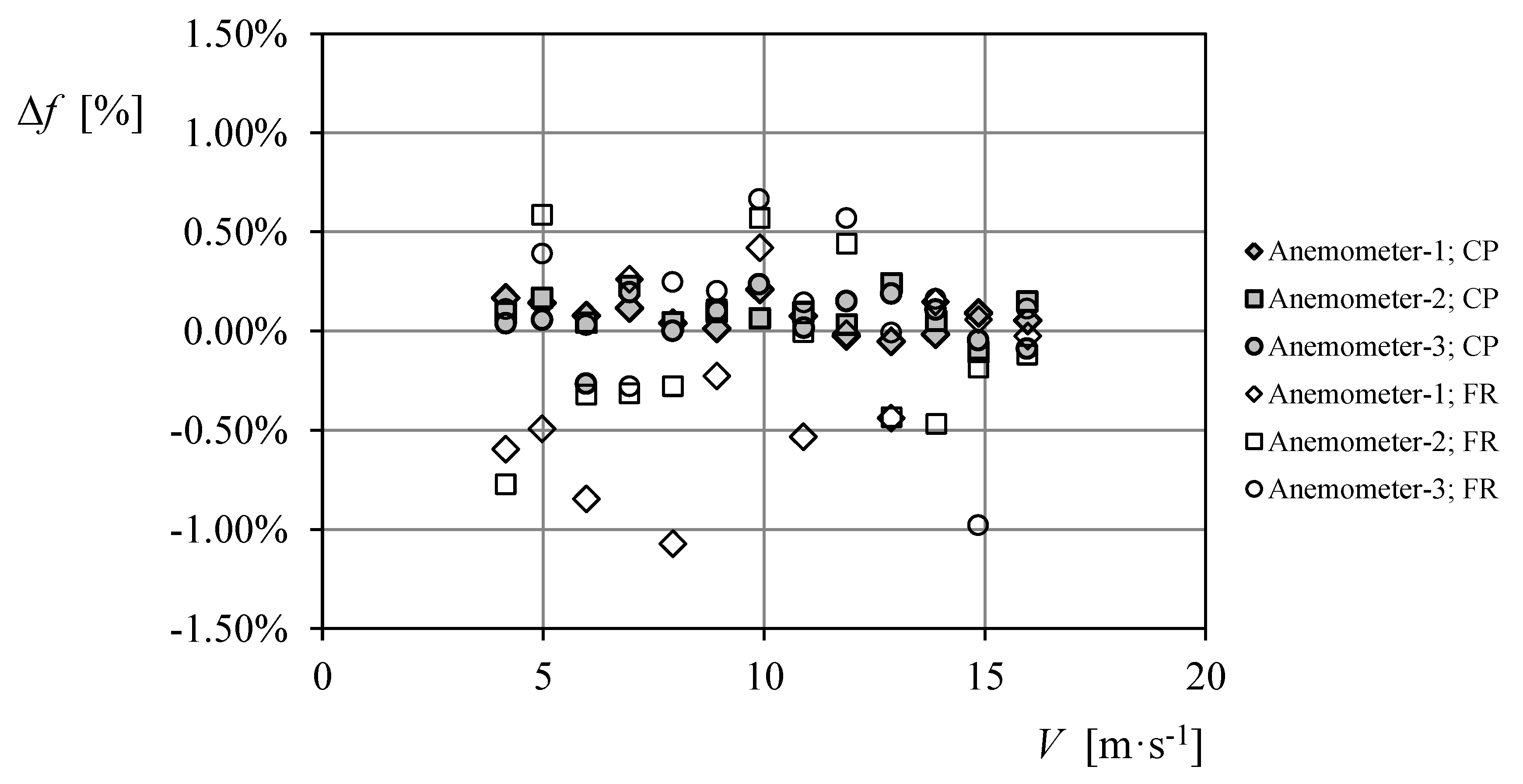
The results of the calibrations performed on the three case study anemometers are included in Table 5. In this table, the calibration coefficients (see Equation (5)) resulting from the accredited calibration system of the IDR/UPM Institute, are compared to the ones from the data recorded with ABDAS, post-processed using both aforementioned procedures, counting pulses (Equation (6)), and using the Fourier transform (Equation (7)). As it can be observed, no big differences seem to be between the calibration constants obtained with the procedures used (see also Figure 17). However, the fitting to the wind speed/frequency data is better correlated to the linear transfer function (Equation (5)) counting pulses than using the Fourier transform, as indicated by the higher values of the correlation coefficient R. Bearing in mind that the frequencies obtained with the IDR/UPM accredited calibration system can be assumed to be the most accurate ones, the two procedures for extraction the anemometer output frequency from the data can be compared in relation to that values. In Figure 18, the percentage difference of the frequencies obtained, f, in relation to the ones measured with the IDR/UPM system, fIDR:
is shown for the three calibrated anemometers. The graph displayed in this figure indicates a larger deviation of the frequencies based on the Fourier transform from the ones calculated with the reference IDR/UPM calibration system. Furthermore, the standard deviation of these data, σ∆f, is included in Table 5, clearly indicating a poorer results of the calibrations performed using the Fourier transform instead of counting the number of pulses within the recording period.
5. Conclusions
A low-cost Arduino-Based Data Acquisition System (ABDAS) for use in the IDR/UPM Institute aerodynamics lab has been designed and developed. This system has proven to be accurate enough to measure signals up to 50 Hz within ±1% error level. Besides, ABDAS has been used to analyze wind sensors (cup anemometers) performance, the most relevant conclusion resulting from this particular case study being:
- ABDAS was able to record data that produce cup anemometer transfer functions similar to the ones obtained with the accredited anemometer calibration system from IDR/UPM;
- The cup anemometer transfer function parameter extraction procedure based on counting pulses, is better than the one based on the Fourier transform in terms of accuracy of the transfer function.
Author Contributions
Data curation, A.V.-P.; Formal analysis, S.P.; Methodology, S.P.; Software, A.V.-P.; Validation, A.V.-P. and S.P.; Writing–original draft, S.P.
Funding
This research received no external funding.
Acknowledgments
The authors are indebted to Ángel Sanz-Andrés for his kind support regarding the research program Prácticas en Empresa of the Aerospace Eng. Degree at Instituto Universitario de Microgravedad “Ignacio Da Riva” (IDR/UPM). Furthermore, authors would like to express their gratitude to the IDR/UPM staff and colleagues for the kind help regarding the testing campaigns carried out to obtain the results described in this work. The support from Enrique Vega and Luis García should be especially mentioned.
Conflicts of Interest
The authors declare no conflict of interest.
References
- Pindado, S.; Meseguer, J. Wind tunnel study on the influence of different parapets on the roof pressure distribution of low-rise buildings. J. Wind Eng. Ind. Aerodyn. 2003, 91, 1133–1139. [Google Scholar] [CrossRef] [Green Version]
- Pindado, S.Ã.; Meseguer, J.; Franchini, S. The influence of the section shape of box-girder decks on the steady aerodynamic yawing moment of double cantilever bridges under construction. J. Wind Eng. Ind. Aerodyn. 2005, 93, 547–555. [Google Scholar] [CrossRef] [Green Version]
- Franchini, S.; Pindado, S.; Meseguer, J. A parametric, experimental analysis of conical vortices on curved roofs of low-rise buildings. J. Wind Eng. Ind. Aerodyn. 2005, 93, 639–650. [Google Scholar] [CrossRef] [Green Version]
- Pindado, S.; Meseguer, J.; Franchini, S. Influence of an upstream building on the wind-induced mean suction on the flat roof of a low-rise building. J. Wind Eng. Ind. Aerodyn. 2011, 99, 889–893. [Google Scholar] [CrossRef] [Green Version]
- Avila-Sanchez, S.; Pindado, S.; Lopez-Garcia, O.; Sanz-Andres, A. Wind tunnel analysis of the aerodynamic loads on rolling stock over railway embankments: The effect of shelter windbreaks. Sci. World J. 2014. [Google Scholar] [CrossRef] [PubMed]
- Meseguer, J.; Sanz-Andres, A.G.A.; Sanz-Andrés, A.; Alonso, G. Determination of Maximum Mechanical Energy Efficiency in Energy Galloping Systems. J. Eng. Mech. 2015, 141, 04014101. [Google Scholar] [CrossRef] [Green Version]
- Ogueta-Gutiérrez, M.; Franchini, S.; Alonso, G. Effects of bird protection barriers on the aerodynamic and aeroelastic behaviour of high speed train bridges. Eng. Struct. 2014, 81, 22–34. [Google Scholar] [CrossRef]
- García, E.T.; Ogueta-gutiérrez, M.; Ávila, S.; Franchini, S.; Herrera, E.; Meseguer, J. On the effects of windbreaks on the aerodynamic loads over parabolic solar troughs. Appl. Energy 2014, 115, 293–300. [Google Scholar] [CrossRef] [Green Version]
- Ghaemi-Nasab, M.; Davari, A.R.; Franchini, S. A new approach to correct yaw misalignment in the spinning ultrasonic anemometer. Meas. Sci. Technol. 2018, 29, 015001. [Google Scholar] [CrossRef]
- Ghaemi-Nasab, M.; Franchini, S.; Davari, A.R. A procedure for calibrating the spinning ultrasonic wind sensors. Measurement 2018, 114, 365–371. [Google Scholar] [CrossRef]
- Pindado, S.; Vega, E.; Martínez, A.; Meseguer, E.; Franchini, S.; Pérez Sarasola, I. Analysis of calibration results from cup and propeller anemometers. Influence on wind turbine Annual Energy Production (AEP) calculations. Wind Energy 2010, 14, 119–132. [Google Scholar] [CrossRef]
- Pindado, S.; Sanz, A.; Wery, A. Deviation of cup and propeller anemometer calibration results with air density. Energies 2012, 5, 683–701. [Google Scholar] [CrossRef]
- Pindado, S.; Barrero-Gil, A.; Sanz, A. Cup anemometers’ loss of performance due to ageing processes, and its effect on Annual Energy Production (AEP) estimates. Energies 2012, 5, 1664–1685. [Google Scholar] [CrossRef] [Green Version]
- Pindado, S.; Pérez, J.; Avila-Sanchez, S. On cup anemometer rotor aerodynamics. Sensors 2012, 12, 6198–6217. [Google Scholar] [CrossRef] [PubMed] [Green Version]
- Pindado, S.; Pérez, I.; Aguado, M. Fourier analysis of the aerodynamic behavior of cup anemometers. Meas. Sci. Technol. 2013, 24, 065802. [Google Scholar] [CrossRef]
- Pindado, S.; Cubas, J.; Sanz-Andrés, Á. Aerodynamic analysis of cup anemometers performance: The stationary harmonic response. Sci. World J. 2013, 2013. [Google Scholar] [CrossRef] [PubMed]
- Vega, E.; Pindado, S.; Martínez, A.; Meseguer, E.; García, L. Anomaly detection on cup anemometers. Meas. Sci. Technol. 2014, 25, 127002. [Google Scholar] [CrossRef] [Green Version]
- Sanz-Andrés, Á.; Pindado, S.; Sorribes-Palmer, F. Mathematical analysis of the effect of rotor geometry on cup anemometer response. Sci. World J. 2014, 2014. [Google Scholar] [CrossRef] [PubMed]
- Pindado, S.; Cubas, J.; Sorribes-Palmer, F. On the harmonic analysis of cup anemometer rotation speed: A principle to monitor performance and maintenance status of rotating meteorological sensors. Measurement 2015, 73, 401–418. [Google Scholar] [CrossRef] [Green Version]
- Pindado, S.; Ramos-Cenzano, A.; Cubas, J. Improved analytical method to study the cup anemometer performance. Meas. Sci. Technol. 2015, 26, 107001. [Google Scholar] [CrossRef] [Green Version]
- Martínez, A.; Vega, E.; Pindado, S.; Meseguer, E.; García, L. Deviations of cup anemometer rotational speed measurements due to steady state harmonic accelerations of the rotor. Meas. J. Int. Meas. Confed. 2016, 90, 483–490. [Google Scholar] [CrossRef] [Green Version]
- Roibas-Millan, E.; Cubas, J.; Pindado, S. Studies on cup anemometer performances carried out at IDR/UPM Institute. Past and present research. Energies 2017, 10, 1860. [Google Scholar] [CrossRef]
- Cubas, J.; Pindado, S.; De Manuel, C. Explicit expressions for solar panel equivalent circuit parameters based on analytical formulation and the lambert W-function. Energies 2014, 7, 4098–4115. [Google Scholar] [CrossRef]
- Cubas, J.; Pindado, S.; Victoria, M. On the analytical approach for modeling photovoltaic systems behavior. J. Power Sources 2014, 247, 467–474. [Google Scholar] [CrossRef] [Green Version]
- Cubas, J.; Farrahi, A.; Pindado, S. Magnetic Attitude Control for Satellites in Polar or Sun-Synchronous Orbits. J. Guid. Control Dyn. 2015, 38, 1947–1958. [Google Scholar] [CrossRef]
- Roibás-Millán, E.; Alonso-Moragón, A.; Jiménez-Mateos, A.G.; Pindado, S. Testing solar panels for small-size satellites: The UPMSAT-2 mission. Meas. Sci. Technol. 2017, 28, 115801. [Google Scholar] [CrossRef]
- Pindado, S.; Cubas, J. Simple mathematical approach to solar cell/panel behavior based on datasheet information. Renew. Energy 2017, 103, 729–738. [Google Scholar] [CrossRef] [Green Version]
- Pindado, S.; Cubas, J.; Roibás-Millán, E.; Sorribes-Palmer, F. Project-based learning applied to spacecraft power systems: A long-term engineering and educational program at UPM University. CEAS Space J. 2018, 1–17. [Google Scholar] [CrossRef]
- Torralbo, I.; Perez-Grande, I.; Sanz-Andres, A.; Piqueras, J. Correlation of spacecraft thermal mathematical models to reference data. Acta Astronaut. 2018, 144, 305–319. [Google Scholar] [CrossRef]
- Fernández-Rico, G.; Pérez-Grande, I.; Sanz-Andres, A.; Torralbo, I.; Woch, J. Quasi-autonomous thermal model reduction for steady-state problems in space systems. Appl. Therm. Eng. 2016, 105, 456–466. [Google Scholar] [CrossRef] [Green Version]
- Pérez Grande, I.; Torralbo, I.; Alonso, G.; Gómez-Sanjuan, A.; Fernandez-Rico, G. Thermal Design of the ESA Solar Orbiter Instrument PHI. In Proceedings of the 46th International Conference on Environmental Systems, Vienna, Austria, 10–14 July 2016; pp. 1–11. [Google Scholar]
- Pérez Grande, I.; Peinado, L.; Chamorro, A.; Torralbo, I.; Alonso, G.; Rodriguez Manfredi, J.A.; Lepinette, A.; Sebastián, E. Thermal design of the Air Temperature Sensor (ATS) and the Thermal InfraRed Sensor (TIRS) of the Mars Environmental Dynamics Analyzer (MEDA) for Mars 2020. In Proceedings of the 47th International Conference on Environmental Systems, Charleston, SC, USA, 16–20 July 2017. [Google Scholar]
- Fisher, D.K.; Gould, P.J. Open-Source Hardware Is a Low-Cost Alternative for Scientific Instrumentation and Research. Mod. Instrum. 2012, 1, 8–20. [Google Scholar] [CrossRef]
- Pardyjak, E.R.; Stoll, R. Improving measurement technology for the design of sustainable cities. Meas. Sci. Technol. 2017, 28, 092001. [Google Scholar] [CrossRef]
- González, A.; Olazagoitia, J.L.; Vinolas, J. A low-cost data acquisition system for automobile dynamics applications. Sensors 2018, 18, 366. [Google Scholar] [CrossRef] [PubMed]
- Andria, G.; Attivissimo, F.; Di Nisio, A.; Lanzolla, A.M.L.; Pellegrino, A. Development of an automotive data acquisition platform for analysis of driving behavior. Measurement 2016, 93, 278–287. [Google Scholar] [CrossRef]
- Erraissi, N.; Raoufi, M.; Aarich, N.; Akhsassi, M.; Bennouna, A. Implementation of a low-cost data acquisition system for “PROPRE.MA” project. Measurement 2018, 117, 21–40. [Google Scholar] [CrossRef]
- Stornelli, V.; Ferri, G.; Leoni, A.; Pantoli, L. The assessment of wind conditions by means of hot wire sensors and a modifed Wheatstone bridge architecture. Sens. Actuators A Phys. 2017, 262, 130–139. [Google Scholar] [CrossRef]
- Srividyadevi, P.; Pusphalatha, D.V.; Sharma, P.M. Measurement of Power and Energy Using Arduino. Res. J. Eng. Sci. 2013, 2, 10–15. [Google Scholar]
- Mnati, M.J.; Van den Bossche, A.; Chisab, R.F. A smart voltage and current monitoring system for three phase inverters using an android smartphone application. Sensors 2017, 17, 872. [Google Scholar] [CrossRef] [PubMed]
- Rao, A.S. Design of Low-cost Autonomous Water Quality Monitoring System. In Proceedings of the International Conference on Advances in Computing, Communications and Informatics (ICACCI), Mysore, India, 22–25 August 2013; pp. 14–19. [Google Scholar]
- Fuentes, M.; Vivar, M.; Burgos, J.M.; Aguilera, J.; Vacas, J.A. Design of an accurate, low-cost autonomous data logger for PV system monitoring using ArduinoTM that complies with IEC standards. Sol. Energy Mater. Sol. Cells 2014, 130, 529–543. [Google Scholar] [CrossRef]
- Mahzan, N.N.; Omar, A.M.; Rimon, L.; Noor, S.Z.M.; Rosselan, M.Z. Design and development of an arduino based data logger for photovoltaic monitoring system. Int. J. Simul. Syst. Sci. Technol. 2017, 17, 15.1–15.5. [Google Scholar] [CrossRef]
- Zachariadou, K.; Yiasemides, K.; Trougkakos, N. A low-cost computer-controlled Arduino-based educational laboratory system for teaching the fundamentals of photovoltaic cells. Eur. J. Phys. 2012, 33, 1599–1610. [Google Scholar] [CrossRef]
- Hertzog, P.E.; Swart, A.J. A customizable energy monitoring system for renewable energy systems. In Proceedings of the 23rd Southern African Universities Power Engineering Conference (SAUPEC 2015), Johannesburg, South Africa, 28–30 January 2015; pp. 154–159. [Google Scholar]
- Abtahi, F.; Aslamy, B.; Boujabir, I.; Seoane, F.; Lindecrantz, K. An Affordable ECG and Respiration Monitoring System Based on Raspberry PI and ADAS1000: First Step towards Homecare Applications. In Proceedings of the 16th Nordic-Baltic Conference on Biomedical Engineering, Gothenburg, Sweden, 14–16 October 2014; Springer: Cham, Switzerland, 2015; Volume 48, pp. 5–9. [Google Scholar] [CrossRef]
- Kemis, H.; Bruce, N.; Ping, W.; Antonio, T.; Gook, L.B.; Lee, H.J. Healthcare monitoring application in ubiquitous sensor network: Design and implementation based on pulse sensor with arduino. In Proceedings of the 6th International Conference on New Trends in Information Science, Service Science and Data Mining (ISSDM2012), Taipei, Taiwan, 23–25 October 2012; pp. 34–38. [Google Scholar]
- Butca, C.G.; Suciu, G.; Ochian, A.; Fratu, O.; Halunga, S. Wearable sensors and cloud platform for monitoring environmental parameters in e-health applications. In Proceedings of the 11th International Symposium on Electronics and Telecommunications (ISETC), Timisoara, Romania, 14–15 November 2014. [Google Scholar] [CrossRef]
- Alemán-soler, N.M.; Travieso, C.M.; Guerra-segura, E.; Alonso, J.B. Biometric Approach Based on Physiological Human Signals. In Proceedings of the 3rd International Conference on Signal Processing and Integrated Networks (SPIN), Noida, India, 11–12 February 2016; pp. 681–686. [Google Scholar]
- Molina-Cantero, A.J.; Castro-García, J.A.; Lebrato-Vázquez, C.; Gómez-González, I.M.; Merino-Monge, M. Real-time processing library for open-source hardware biomedical sensors. Sensors 2018, 18, 1033. [Google Scholar] [CrossRef] [PubMed]
- Sumathi, M.; Ranjan, R.; Singh, R.K.; Kumar, P. Performance analysis of sun sensors for satellite systems. In Proceedings of the International Conference on Advanced Electronic Systems (ICAES 2013), Pilani, India, 21–23 September 2013; pp. 10–14. [Google Scholar]
- Abo-arais, M.; Elfeki, M.; El-mohr, M.; Abdelmoteleb, B.; Hatem, A.; Mohamed, A.; Ramy, A.; Walid, K.; El-fiky, M.; Darwish, A.; et al. Approaching a nano-satellite using CAN-SAT systems. In Proceedings of the 7th International Conference on Recent Advances in Space Technologies (RAST), Istanbul, Turkey, 16–19 June 2015; pp. 813–817. [Google Scholar]
- Laskar, M.R.; Bhattacharjee, R.; Giri, M.S.; Bhattacharya, P. Weather Forecasting using Arduino Based Cube-Sat. Procedia Comput. Sci. 2016, 89, 320–323. [Google Scholar] [CrossRef]
- Clarke, M.; Guo, J.; Sanders, B.; Gasiewski, A. Affordable and Accessible Attitude Control Validation Test Methods for CubeSats. In Proceedings of the 67th International Astronautical Congress (IAC), Guadalajara, Mexico, 26–30 September 2016; pp. 26–30. [Google Scholar]
- Shafique, A.; Shabir, A.; Sharif, Z.; Shabbir, N.; Iqbal, M.N. Power Distribution System for PNSS-1 Cubical Satellite. In Proceedings of the ISNET/SUPARCO Workshop on Student Satellites, Lahore, Pakistan, 2–6 November 2015. [Google Scholar]
- Sarik, J.; Kymissis, I. Lab Kits Using the Arduino Prototyping Platform. In Proceedings of the IEEE Frontiers in Education Conference (FIE), Washington, DC, USA, 27–30 October 2010; pp. 1–5. [Google Scholar]
- Enikov, E.; Eke, E. Teaching Classical Control System Course With Portable Student-Owned Mechatronic Kits. In Proceedings of the ASME International Mechanical Engineering Congress and Exposition, Houston, TX, USA, 9–15 November 2012; Volume 5, pp. 509–516. [Google Scholar]
- Sobota, J.; Pisl, R.; Balda, P.; Schlegel, M. Raspberry Pi and Arduino boards in control education. IFAC Proc. Vol. 2013, 10, 7–12. [Google Scholar] [CrossRef]
- Barber, R.; Horra, M.; Crespo, J. Control Practices using Simulink with Arduino as Low Cost Hardware. IFAC Proc. Vol. 2013, 46, 250–255. [Google Scholar] [CrossRef]
- Stark, B.; Li, Z.; Smith, B.C.Y. Take-Home Mechatronics Control Labs: A Low-Cost Personal Solution and Educational Assessment. In Proceedings of the ASME 2013 International Design Engineering Technical Conferences and Computers and Information in Engineering Conference, Portland, OR, USA, 4–7 August 2013. [Google Scholar] [CrossRef]
- Gawad, A.F.A.; Ghulman, H.A.; Mandourah, T.S. Design, Construction and Operation of Unmanned Ship Model for Multidisciplinary Engineering Education. In Proceedings of the Eleventh International Conference of Fluid Dynamics, Alexandria, Egypt, 19–21 December 2013; pp. 1–11. [Google Scholar]
- Soriano, A.; Marín, L.; Vallés, M.; Valera, A.; Albertos, P. Low Cost Platform for Automatic Control Education Based on Open Hardware. IFAC Proc. Vol. 2014, 47, 9044–9050. [Google Scholar] [CrossRef]
- Chancharoen, R.; Sripakagorn, A.; Maneeratana, K. An Arduino kit for learning mechatronics and its scalability in semester projects. In Proceedings of the IEEE International Conference on Teaching, Assessment and Learning for Engineering (TALE), Wellington, New Zealand, 8–10 December 2014; pp. 505–510. [Google Scholar] [CrossRef]
- Reck, R.M.; Sreenivas, R.S. Developing an afforable laboratory kit for undergraduate controls education. In Proceedings of the ASME 2014 Dynamic Systems and Control Conference, San Antonio, TX, USA, 22–24 October 2014; pp. 1–9. [Google Scholar]
- Reguera, P.; García, D.; Domínguez, M.; Prada, M.A.; Alonso, S. A Low-cost Open Source Hardware in Control Education. Case Study: Arduino-Feedback Ms-150. IFAC-PapersOnLine 2015, 48, 117–122. [Google Scholar] [CrossRef]
- Reck, R.M.; Sreenivas, R.S.; Loui, M.C. Assessing an affordable and portable laboratory kit in an undergraduate control systems course. In Proceedings of the IEEE Frontiers in Education Conference (FIE), El Paso, TX, USA, 21–24 October 2015; pp. 1–4. [Google Scholar]
- Hassanpour, P. Design, Implementation, and Incorporation of a Control System Platform in an Undergraduate- Level Control Systems Course. In Proceedings of the ASME 2017 International Mechanical Engineering Congress and Exposition, Tampa, FL, USA, 3–9 November 2017. [Google Scholar] [CrossRef]
- Pindado, S.; Sanz Andres, A.; Franchini, S.; Pérez Grande, I.; Alonso, G.; Pérez-Alvarez, J.; Sorribes-Palmer, F.; Cubas, J.; García, A.; Roibás-Millán, E.; et al. MUSE (Master in Space Systems), an Advanced Master’s Degree in Space Engineering. In Proceedings of the 1st Annual International Conference on Engineering Education & Teaching, Athens, Greece, 9–12 May 2016; pp. 1–16. [Google Scholar]
- Pindado, S.; Roibas-Millan, E.; Cubas, J.; García, A.; Sanz-Andres, A.; Franchini, S.; Pérez-Grande, I.; Alonso, G.; Pérez-Álvarez, J.; et al. The UPMSat-2 Satellite: An Academic Project within Aerospace Engineering Education. In Proceedings of the 2nd Annual International Conference on Engineering Education & Teaching, Athens, Greece, 5–8 June 2017; pp. 1–28. [Google Scholar]
- Arduino. Arduino Mega 2560. 2014. Available online: https://www.arduino.cc/ (accessed on 21 July 2017).
Figure 1.
Diagram of the Arduino-Based Data Acquisition System (ABDAS) described in the present work.
Figure 1.
Diagram of the Arduino-Based Data Acquisition System (ABDAS) described in the present work.

Figure 2.
Sketch of the voltage dividers used to enlarge the measuring rang of ABDAS.

Figure 3.
Transfer function (Equation (2)) of ABDAS voltage dividers. The Equation (linear fitting) correspondent to Channel-1 voltage divider (VD-1) is included in the Figure. See also Table 2.
Figure 3.
Transfer function (Equation (2)) of ABDAS voltage dividers. The Equation (linear fitting) correspondent to Channel-1 voltage divider (VD-1) is included in the Figure. See also Table 2.

Figure 4.
Pictures of ABDAS along its development/manufacturing process. (a) Connectors, lightning and switching panel. (b) ABDAS distribution inside the enclosure. (c) Front view. (d) Rear view.
Figure 4.
Pictures of ABDAS along its development/manufacturing process. (a) Connectors, lightning and switching panel. (b) ABDAS distribution inside the enclosure. (c) Front view. (d) Rear view.

Figure 5.
ABDAS software flowchart. Program steps and measurement loop.

Figure 6.
Image capture with part of the ABDAS software control program code.

Figure 7.
Serial monitor window of ABDAS.

Figure 8.
Results from a measurement carried out with ABDAS. Text file example. Two channels measured (two first column). The third column indicates the time of each measurement point (expressed in seconds).
Figure 8.
Results from a measurement carried out with ABDAS. Text file example. Two channels measured (two first column). The third column indicates the time of each measurement point (expressed in seconds).

Figure 9.
Arduino-based acquisition system (ABDAS) and the National Instruments NI USB-6210 data acquisition system (NIDAS), used to check its performances.
Figure 9.
Arduino-based acquisition system (ABDAS) and the National Instruments NI USB-6210 data acquisition system (NIDAS), used to check its performances.

Figure 10.
One wave period of the 10 Hz frequency reference signal (Equation (3)). The data measured with NIDAS and ABDAS have been included for comparison purposes.
Figure 10.
One wave period of the 10 Hz frequency reference signal (Equation (3)). The data measured with NIDAS and ABDAS have been included for comparison purposes.

Figure 11.
Sketch of the S4 wind tunnel at the IDR/UPM Institute used for anemometer calibration. The different parts of the wind tunnel are indicated in the figure as follows: 1. Fans; 2. Plenum chamber; 3. Honeycomb and grids; 4. Contraction; 5. Test chamber; 6. Diffuser. [11].
Figure 11.
Sketch of the S4 wind tunnel at the IDR/UPM Institute used for anemometer calibration. The different parts of the wind tunnel are indicated in the figure as follows: 1. Fans; 2. Plenum chamber; 3. Honeycomb and grids; 4. Contraction; 5. Test chamber; 6. Diffuser. [11].

Figure 12.
Offset, y0, and the first harmonic term, y1, extracted from the sampled data of same signal (Equation (3)) measured with NIDAS and ABDAS.
Figure 12.
Offset, y0, and the first harmonic term, y1, extracted from the sampled data of same signal (Equation (3)) measured with NIDAS and ABDAS.

Figure 13.
Harmonic terms, y2 to y10, extracted from the sampled data of same signal (Equation (3)) measured with NIDAS and ABDAS.
Figure 13.
Harmonic terms, y2 to y10, extracted from the sampled data of same signal (Equation (3)) measured with NIDAS and ABDAS.

Figure 14.
Estimated accuracy ABDAS and NIDAS in relation to the frequency of the signal measured (Equation (3)).
Figure 14.
Estimated accuracy ABDAS and NIDAS in relation to the frequency of the signal measured (Equation (3)).

Figure 15.
Number sample points (open circles) measured with ABDAS into three 2-period brackets of the three tested cup anemometers’ output signal.
Figure 15.
Number sample points (open circles) measured with ABDAS into three 2-period brackets of the three tested cup anemometers’ output signal.

Figure 16.
Fourier transforms of the recording data with ABDAS during the calibration process of Anemometer-2, at 4 and 16 m·s−1.
Figure 16.
Fourier transforms of the recording data with ABDAS during the calibration process of Anemometer-2, at 4 and 16 m·s−1.

Figure 17.
Calibration points of Anemometer-1, obtained from the IDR/UPM calibration system (the transfer function resulting from these data is included in the graph), and from the data measured with ABDAS and post-processed counting pulses (ABDAS-CP; see Equation (6)) and using the Fourier transform (ABDAS-FR; see Equation (7)).

Figure 18.
Percentage difference of the frequencies obtained, ∆f (Equation (8)), from the ABDAS data measurements using the pulse-counting (CP; Equation (6)) and the Fourier transform (FR; Equation (7)) procedures, related to the ones measured with the IDR/UPM system, fIDR.
Figure 18.
Percentage difference of the frequencies obtained, ∆f (Equation (8)), from the ABDAS data measurements using the pulse-counting (CP; Equation (6)) and the Fourier transform (FR; Equation (7)) procedures, related to the ones measured with the IDR/UPM system, fIDR.


Table 1.
Technical specifications of Arduino Mega 2560 [70].
Table 1.
Technical specifications of Arduino Mega 2560 [70].
| Microcontroller | ATmega 2560 |
|---|---|
| Operating Voltage | 5 V |
| Input Voltage (recommended) | 7–12 V |
| Input Voltage (limit) | 6–20 V |
| Digital I/O Pins | 54 (of which 15 provide PWM output) |
| Analog Input Pins | 16 |
| DC Current per I/O Pin | 20 mA |
| DC Current for 3.3 V Pin | 50 mA |
| Flash Memory | 256 KB (8 KB used by bootloader) |
| SRAM | 8 KB |
| EEPROM | 4 KB |
| Clock Speed | 16 MHz |
| LED_BUILTIN | 13 |
| Length | 101.52 mm |
| Width | 53.3 mm |
Table 2.
Transfer function coefficients, a and b, of the voltage divider installed at each ABDAS input channel. The coefficient of determination, R2, corresponding to the fitting (see Figure 3) are included, together with the maximum and averaged error, |ε|max and |ε|avg, between the measurements (Figure 3) and the transfer function.
| Voltage Divider | a | b [V] | R2 | |ε|max [V] | |ε|avg [V] |
|---|---|---|---|---|---|
| VD-1 | 0.66684 | −0.00101 | 1.0 | 2.5320 × 10⁻³ | 8.4159 × 10⁻⁴ |
| VD-2 | 0.66413 | −0.00037 | 1.0 | 1.2941 × 10⁻³ | 6.8456 × 10⁻⁴ |
| VD-3 | 0.66810 | −0.00066 | 1.0 | 1.3404 × 10⁻³ | 5.3216 × 10⁻⁴ |
| VD-4 | 0.66696 | −0.00055 | 1.0 | 1.5693 × 10⁻³ | 5.7317 × 10⁻⁴ |
| VD-5 | 0.66622 | −0.00005 | 1.0 | 1.7064 × 10⁻³ | 6.0411 × 10⁻⁴ |
Table 3.
Characteristics and price of ABDAS components.
| Component | Nature | Commercial | Price [€] |
|---|---|---|---|
| Arduino Mega 2560 | Obligatory | Yes | 42 |
| BNC | Obligatory | Yes | 8.65 |
| Switches | Optional | Yes | 7.45 |
| Enclosure | Obligatory | Yes | 11.11 |
| Resistor | Obligatory | Yes | 8.2 |
| Battery holders | Optional | Yes | 7.5 |
| Batteries | Optional | Yes | 6.2 |
| Cable & welding | Obligatory | No | 3.5 |
| Leds | Optional | Yes | 7.85 |
| Switching button | Obligatory | Yes | 0.79 |
Table 4.
Number of points, nw, measured by NIDAS and ABDAS in one single period of the reference signal, and highest Fourier harmonic term, ymax, able to be correctly extracted.
Table 4.
Number of points, nw, measured by NIDAS and ABDAS in one single period of the reference signal, and highest Fourier harmonic term, ymax, able to be correctly extracted.
| Reference signal (Sine-Wave) Frequency | NIDAS | ABDAS | ||
|---|---|---|---|---|
| nw | ymax | nw | ymax | |
| 10 Hz | 500 | y249 | 83–84 | y41 |
| 50 Hz | 400 | y49 | 16–17 | y8 |
| 100 Hz | 50 | y24 | 8–9 | y4 |
| 250 Hz | 20 | y9 | 3–4 | y1 |
Table 5.
Calibration coefficients, A, B, and correlation coefficient R, (see Equation (5)) resulting from the calibrations performed to Anemometers 1–3. The coefficients included in the table are the ones obtained from the IDR/UPM accredited calibration process, and the ones from the data measured with ABDAS and post-processed counting pulses (ABDAS-CP; see Equation (6)) and using the Fourier transform (ABDAS-FR; see Equation (7)).
| Anemometer 1 | |||
| Calibration Constants | IDR/UPM Cal. Sys | ABDAS-CP | ABDAS-FR |
| A [m] | 0.04584 | 0.04584 | 0.04572 |
| B [m·s−1] | 0.2704 | 0.2635 | 0.3128 |
| R | 0.99999 | 0.99998 | 0.99992 |
| σ∆f | - | 7.790 × 10⁻⁴ | 4.467 × 10⁻³ |
| Anemometer 2 | |||
| Calibration Constants | IDR/UPM Cal. Sys | ABDAS-CP | ABDAS-FR |
| A [m] | 0.04604 | 0.04602 | 0.04613 |
| B [m·s−1] | 0.2449 | 0.2404 | 0.2348 |
| R | 0.99999 | 0.99999 | 0.99990 |
| σ∆f | - | 9.111 × 10⁻⁴ | 4.128 × 10⁻³ |
| Anemometer 3 | |||
| Calibration Constants | IDR/UPM Cal. Sys | ABDAS-CP | ABDAS-FR |
| A [m] | 0.04590 | 0.04589 | 0.04602 |
| B [m·s−1] | 0.2604 | 0.2568 | 0.2279 |
| R | 0.99999 | 0.99999 | 0.99987 |
| σ∆f | - | 1.366 × 10⁻³ | 4.068 × 10⁻³ |
© 2018 by the authors. Licensee MDPI, Basel, Switzerland. This article is an open access article distributed under the terms and conditions of the Creative Commons Attribution (CC BY) license (http://creativecommons.org/licenses/by/4.0/).
Share and Cite
MDPI and ACS Style
Vidal-Pardo, A.; Pindado, S. Design and Development of a 5-Channel Arduino-Based Data Acquisition System (ABDAS) for Experimental Aerodynamics Research. Sensors 2018, 18, 2382. https://doi.org/10.3390/s18072382
AMA Style
Vidal-Pardo A, Pindado S. Design and Development of a 5-Channel Arduino-Based Data Acquisition System (ABDAS) for Experimental Aerodynamics Research. Sensors. 2018; 18(7):2382. https://doi.org/10.3390/s18072382
Chicago/Turabian StyleVidal-Pardo, Antonio, and Santiago Pindado. 2018. "Design and Development of a 5-Channel Arduino-Based Data Acquisition System (ABDAS) for Experimental Aerodynamics Research" Sensors 18, no. 7: 2382. https://doi.org/10.3390/s18072382
Note that from the first issue of 2016, this journal uses article numbers instead of page numbers. See further details here.