Sensor Fusion of Monocular Cameras and Laser Rangefinders for Line-Based Simultaneous Localization and Mapping (SLAM) Tasks in Autonomous Mobile Robots

Abstract

This paper presents a sensor fusion strategy applied for Simultaneous Localization and Mapping (SLAM) in dynamic environments. The designed approach consists of two features: (i) the first one is a fusion module which synthesizes line segments obtained from laser rangefinder and line features extracted from monocular camera. This policy eliminates any pseudo segments that appear from any momentary pause of dynamic objects in laser data. (ii) The second characteristic is a modified multi-sensor point estimation fusion SLAM (MPEF-SLAM) that incorporates two individual Extended Kalman Filter (EKF) based SLAM algorithms: monocular and laser SLAM. The error of the localization in fused SLAM is reduced compared with those of individual SLAM. Additionally, a new data association technique based on the homography transformation matrix is developed for monocular SLAM. This data association method relaxes the pleonastic computation. The experimental results validate the performance of the proposed sensor fusion and data association method.

1. Introduction

A crucial characteristic of an autonomous mobile robot is its ability to determine its whereabouts and make sense of its static and dynamic environments. The central question of perception of its position in known and unknown world has received great attention in robotics research community. Mapping, localization, and particularly their integration in the form of Simultaneous Localization and Mapping (SLAM) is the basic ability with which other advanced tasks such as exploration and autonomous navigation can be successfully implemented. Therefore, SLAM has been vigorously pursued in the mobile robot research field.

Monocular cameras have been widely used as low cost sensors in numerous robotics applications in recent years. They provide the autonomous mobile robot with abundant information that facilitates intuitive interpretation and comprehension of the environment better than other scanning sensors. The algorithms based on monocular cameras perform reasonable visual SLAM procedures. Points/landmarks extracted from images are common map elements and typically present in structured indoor scenes [1–5]. However, they are easily occluded in dynamic environments if sufficient precautions are not devised. Features of the segment-based map consist of lines and edges which are stable compared with point features and consequently robust enough to improve the performance of the monocular SLAM [6–9]. Most of relevant research above, however, implemented SLAM in static spaces or environments with few moving objects. Dynamic objects induce spurious features and make it difficult to obtain the correct estimates of the robot pose and feature positions. Additionally, erroneously extracted map features corresponding to dynamic objects may lead to inappropriate robot actions that ultimately result in failure to complete the expected tasks.

In this study, we present a sensor fusion strategy for line-based SLAM applied in dynamic environments. This approach fuses the sensor information obtained from a monocular camera and laser rangefinder and includes two modules. One is a feature fusion that integrates the lines extracted respectively from a monocular camera and a laser to remove the erroneous features corresponding to dynamic objects. The other is referred to as a modified multi-sensor point estimation fusion SLAM (MPEF-SLAM) which incorporates two separate EKF SLAM frameworks: monocular and laser SLAM. This modified MPEF-SLAM fuses the state variable and its covariance estimated from individual SLAM procedure and propagates fused values backward to each SLAM process to reduce the error of robot pose and line feature positions. Another advantage of the modified MPEF-SLAM is that its implementation is on the basis of two parallel running SLAM processes, which can avoid unexpected events. For example, when one SLAM procedure does not work due to the sensor failure, the other one can be still running normally. This manifests the idea of redundancy in comparison with the single SLAM framework. Additionally, for monocular SLAM process we suggest a new data association (DA) algorithm. It employs the homography transformation matrix [10] estimated by the matched points determined through Scale Invariant Feature Transform (SIFT) descriptors [11] in two images. The sensor fusion strategy is examined and tested in practical experiments. The results demonstrate that the proposed approach can reliably filter out dynamic aspects and yields accurate models of the environment, as well enhance the localization precision.

The remainder of this paper is organized as follows: after reviewing the related work in Section 2, we elucidate the framework of monocular SLAM and the data association method in Section 3. Section 4 describes the sensor fusion strategy including the feature fusion and modified MPEF-SLAM modules. We validate our proposed methods through the experiments in Section 5. Section 6 gives our conclusions and suggestions for future work.

2. Related Work

Most indoor environments can simply and expediently be represented by line segments. In our previous work [12] and references therein, the line features have been successfully applied to various SLAM algorithms by range scanner sensors. In recent decades, advances in computer vision have provided robotics researchers with efficient and powerful techniques that can be employed in a variety of autonomous tasks. Following Davison and his group’s pioneering work on monocular SLAM [1–5], other researchers studied line-based algorithms. Eade and Drummond [6] proposed an edge-let landmark to depict the line features. This work, which is the extension of the so-called scalable monocular SLAM [4], avoids regions of conflict and deals with multiple matches through robust estimation. Gee and Mayol-Cuevas [7] used fast conic extraction to obtain the 2D edges and then estimated the 3D segments with the Unscented Kalman filter (UKF). Smith et al. [8] applied FAST corners to quickly verify that there was an edge between two corners by bisecting checks. Besides, other researchers conducted similar studies on line based SLAM with a single camera. Lemaire and Lacroix [9] as well as Sola et al. [13] introduced the Plücker coordinates for 3D line description and considered constraints associated with Plücker representation during the updating stage of Kalman filter. Folkesson et al. [14] suggested a M-space feature representation similar to SP-model. This feature model is a general and systematic technique that makes it possible to change sensors and features without any variation to SLAM implementation. In addition, lines and points can be merged to enhance the performance of visual SLAM and improve the precision of the localization and mapping [15,16]. The vertical and the floor lines can also be combined to represent the environment in a more complete fashion via a unified EKF framework by integrating two different measurement models [17].

To the best of our knowledge, almost all mentioned methods above focus on the visual SLAM in static space or the environments with few dynamic objects. In this study, we re-visit the SLAM problem in a dynamic environment from a sensor fusion viewpoint. This approach incorporates the sensor information of a monocular camera and laser rangefinder to remove the feature outliers related to dynamic objects and enhances the accuracy of the localization.

Computer vision technology makes visual SLAM feasible, and related data association methodology is also an interesting area which has attracted much research attention. In addition to conventional data association algorithms such as Nearest Neighbor [7,8], JCBB [18], etc., several data association methods for visual SLAM has been developed, including Normalized Cross-Correlation (NCC) [19,20], incremental expectation maximization algorithm [21], incremental hierarchical data association based on image similarity [22], homography tracking [23] and those based on the SIFT descriptor. The invariant property of the SIFT descriptor is an important factor for the SIFT based data association method. For example, in [24,25] landmarks are identified by SIFT and represented by keypoint descriptors. These landmarks subsequently are treated as the ideal candidates for robust data association. Gil et al. [26,27] managed the data association with the SIFT features from the pattern classification viewpoint, and the Mahalanobis distance was established by the average SIFT descriptors and a high dimensional covariance matrix. Similarly with pattern recognition technology, object-based SLAM [28] combined the advantages of multi-scale Harris corner detector and the SIFT descriptor for natural object recognition, which provides a correct data association. Also, to enhance the robustness of SIFT descriptor a multi-resolution descriptor was proposed to address the problem that the performance gains diminish when uncertainty about camera position increases [29].

These data association methods using the SIFT technique improve the robustness compared with the NCC and image patches based approaches. With this advantage, we also developed a data association method that does not apply the SIFT descriptor as the map features but rather uses the descriptor to estimate the homography transformation matrix of any two images, and then employs the estimated homography transformation matrix to implement data association.

3. Line Based EKF Monocular SLAM

In this section the outline of the line-based monocular SLAM framework is discussed. We briefly present the camera/robot motion and line measurement model. After that the homography transformation matrix based data association method for monocular SLAM is introduced.

3.1. Camera/Robot Motion Model and Line Measurement Model

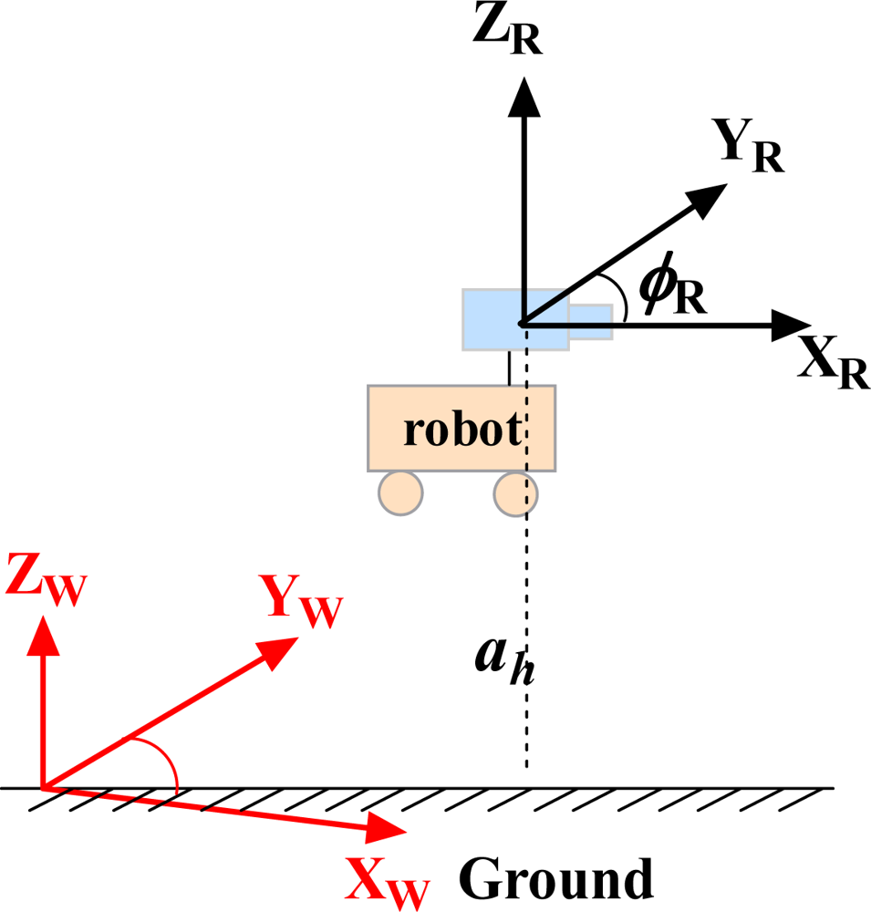
The camera is fixed on the robot platform which moves in a 2D plane, and its translational and rotational velocity are identical with the mobile robot. For convenience, as is shown in Figure 1 we assume the origins of the robot and the camera reference frames are located at the same point.

The simplified camera motion model is:

$${\mathbf{x}}_{v(k)}=\left(\begin{array}{l}{x}_{R(k)}\\ y_{R(k)}\\ {\varphi }_{R(k)}\end{array}\right)=f_v({\mathbf{x}}_{v(k-1)},{\mathbf{u}}_k)=\left(\begin{array}{l}{x}_{R(k-1)}+v_k \text{cos} {\varphi }_k\mathrm{\Delta }t\\ y_{R(k-1)}+v_k \text{sin} {\varphi }_k\mathrm{\Delta }t\\ {\varphi }_{R(k-1)}+{\omega }_k\mathrm{\Delta }t\end{array}\right)$$

(1)

where x_v(k) is the robot pose at time k including the position (x_R(k), y_R(k))^T and head orientation ϕ_R(k); u_k is the control variable at time k including the translation velocity v_k and rotational velocity ω_k; Δt is the sampling time.

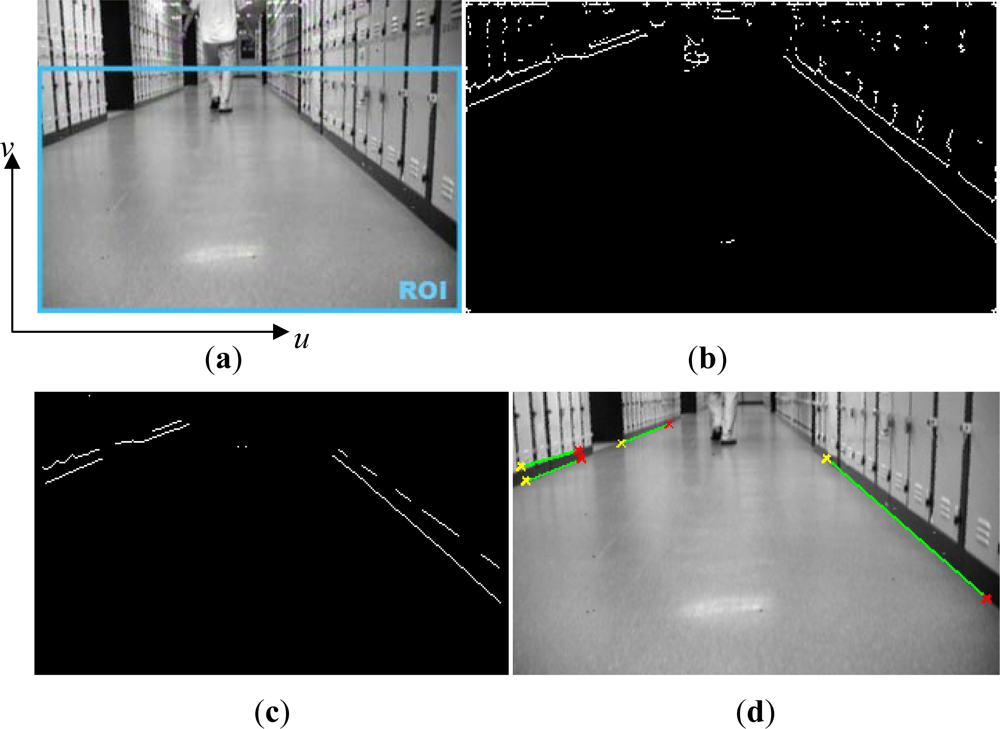
Line extraction is actually an edge detection operation in the image processing terminology. Most of the edge features represented in the related work are extracted by using a first-order edge detection operator: the canny operator [6,7]. In this current study, we employed another first-order edge detector: the Sobel operator combined with a thresholding technique for edge extraction in a specified region of interest (ROI) displayed in Figure 2(a).

The range of ROI encapsulates the ground plane since most static edges are present on the floor. In this ROI we just consider the horizontal static edges, and do not focus on tracking the dynamic targets. After horizontal edge detection processing, it is clear that several edges corresponding to the dynamic objects (i.e., the person here) cannot be eliminated from the selected region, which is illustrated in Figure 2(b). To reduce the effect of these potential outliers, the shrink and clean morphological operations firstly are carried out on all edges. With these operations, the shorter and thinner edges, which usually relate to the parts of dynamic objects, are removed; and secondly for the rest of edges, if the length of an edge is less than the length threshold (in pixels) it is also rejected from the edges set. This operation makes sure to further exclude spurious edges not removed in shrink and clean process (cf. Figure 2(c)). Finally the thicken operation is implemented to recover the interested edges and highlight them (cf. Figure 2(d)), which will prepare for edge parameter extraction in the next step.

We developed two sets of parameters for edge representation: one was used in the measurement model; the other was for data association and sensor fusion. In this subsection, we mainly discuss the parameters for the measurement model. For a line reflected in the vision system, the minimal representation uses four parameters (e.g., Denavit-Hartenberg line coordinates) in 3D Euclidean space but it may be ineffective in some robotic research topics. There are several non-minimal representations for the 3D line, such as endpoints of the line [8], center and unit direction vector of the line [6], two endpoints plus unit direction vectors [7], and so on. In this study, we also describe the lines by the line endpoints non-minimal representation because the advantages are this representation is homogenous and suitable for the projection through a pinhole camera.

Similar to [7,8], with the location of line endpoints we borrowed and extended the idea of their work and presented the line measurement model as:

$${\mathbf{pt}}_{\mathit{mk}}=d_k^m{\mathbf{R}}_{\mathbf{M} k}{\widehat{\mathbf{e}}}_k^m+{\mathbf{x}}_{\mathit{vk}}$$

(2)

$$\left(\begin{array}{l}{h}_k\\ {\phi }_k\end{array}\right)=f({\mathbf{pt}}_{0k},{\mathbf{pt}}_{1k})$$

(3)

$${\mathbf{z}}_k={\left(\begin{array}{ccc}{p}_{\mathit{ek}}& {\varpi }_k& p_{\mathit{ipk}}\end{array}\right)}^T=\mathrm{\Pi }\left({\mathbf{pt}}_{0k},{\mathbf{pt}}_{1k},h_k,{\phi }_k,{\mathbf{P}}_{\mathit{ck}}\right)+n_k$$

(4)

where at step k, in Equation (2)pt_mk is the 3D location of the mth endpoint in the world coordinate system, $d_k^m$ is the depth of the mth endpoint from the camera center, R_Mk is the rotation matrix associated with quaternion, and ${\widehat{\mathbf{e}}}_k^m$ is the unit vector direction of the mth endpoint from the camera center of projection; in Equation (3)h_k is the length of the normal and ϕ_k is the angle of inclination of the normal from the camera/robot framework which will be used for feature fusion, f is the function in matrix form for calculating h_k and ϕ_k; Equation (4) computes the parameters of the 2D line in the image plane. These parameters consist of the measurement variables, including the orientation ϖ_k of the 2D line, the locations of the line’s endpoints p_ek (i.e., pixel coordinates), and coordinates of the projection which is the intersection point p_ipk between a 3D line and the normal of the line (projected intersection point for short in the following sections). Π is the standard pin-hole projection function for a calibrated camera, P_ck is the mean camera projection matrix estimated in the kth step, and n_k is the measurement noise from the image. To make a simple presentation, we define the pixel coordinates of the line endpoints p_ek and projected intersection point p_ipk in a unified form i.e., p = (x_u,y_v)^T. Note that the endpoints initialization is same as the procedure presented by Smith et al. [8].

Besides the location of line’s endpoints used for measurement model, we also considered several additional parameters: the position of projected intersection point p_ip which has been calculated via measurement model and the line descriptor [ρ, θ]^T in Hough space. They are applied as the auxiliary parameters for our proposed data association strategies, and we will concentrate on these topics in the following sections. A step-by-step procedure of the complete edge/line extraction from the camera is as follows:

• Step 1: Pre-process the acquired image to filter out different noise signals;

• Step 2: Select the region of interest (ROI);

• Step 3: In the ROI, detect the horizontal edges by the Sobel operator combined with thresholding;

• Step 4: shrink and clean morphological operations on all edges to eliminate those corresponding to dynamic objects;

• Step 5: Remove the edges whose length is less than the length threshold;

• Step 6: Implement thicken operation to recover the interested edges;

• Step 7: Calculate the pixel coordinates of line endpoints and projected intersection point, and descriptors in Hough space.

3.2. Data Association Based on Homography Transformation Matrix

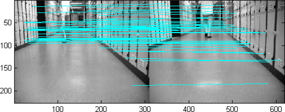
Sampling is considered very important in Nearest Neighbor data association methods. In the reference works [1–5,8], samples in a window region are used to match the predicted features and calculate the innovation. However, the computation pixel by pixel in the predefined region is a little bit repetitious. In this subsection, we suggest a homography transformation matrix based data association (HTMDA) method. This matrix is estimated by the matched points between two images with the help of SIFT descriptors. HTMDA firstly applies the SIFT mechanism to detect the matched points between any two images. Because of advantages of the SIFT, as is shown in Figure 3 the matched points are obviously unsusceptible to the moving object (the person here). Therefore it is reasonable to apply them as the stable points to determine the homography transformation matrix. By these matched points the homography transformation matrix M and its covariance Σ_M can be estimated using the computational procedure of MLE technique [10].

After the estimations of M and Σ_M are obtained, the predicted pixel coordinates p̂^l of line endpoints and projected intersection point in the image plane can be expressed as:

$${\widehat{p}}^l=\mathbf{M}{p}^m$$

(5)

where p^m is the coordinates of the line endpoints and projected intersection point stored in the map (note that projected intersection point is not the component of the state variable). The coordinates of the observed feature in the image is marked as p^l, and the definition of Mahalanobis distance is:

$$s_m={(p^l-{\widehat{p}}^l)}^T{\mathrm{\Sigma }}_{\mathbf{M}}^{-1}(p^l-{\widehat{p}}^l)$$

(6)

When estimating M and Σ_M, we have considered the pixel error in both images as well as the propagation in Equation (5). The covariance in observation and prediction can be regarded as being led by the covariance Σ_M. That is why here we use Σ_M for the Mahalanobis distance computation. As many popular data association algorithms, Mahalanobis distance can be treated as the criteria for data association. Hence in this work, if two values of Mahalonbis distance meet the following condition:

$$s_{\mathit{mi}}\le {\chi }^2(\alpha ,n),i=1,2$$

(7)

(these two Mahalanobis distance values are calculated by any two points, for example two endpoints or one endpoint and one projected intersection point, located on the observed line), then the observed line can be associated with the line stored in the map, labelled as 1, otherwise it is a new feature, marked as 0. Where α is the statistically significant level i.e., P-value and n is the number of degrees of freedom.

Looking back through the implemented process of the proposed HTMDA, compared with the related work in Section 2, instead of directly applying SIFT descriptors as the natural features for data association, we emphasize using the SIFT mechanism to determine the matched points between any two images and then apply these matched points to estimate the homography transformation matrix and its related covariance. The data association is based on this estimated matrix and its covariance. Additionally the main difference between our defined Mahalanobis distance in Equation (6) and the formula in Gil’s work [26] is that the distance is constructed only by Σ_M and the pixel coordinates without any SIFT descriptor.

3.2.1. Practical Considerations on Data Association

Sometimes the position of the predicted image line endpoints may be outside the image range, and we cannot use the criteria (7) above to determine associated features. For this special case, we employ the Hough space parameters presented in previous subsection to handle the data association problem, and adopt an alternative criterion, that is, to test whether the predicted endpoints lie on the observed image lines. The ends lie on the lines if and only if ${\left({\widehat{p}}_h^l\right)}^T{l}^m=0$. We relax this condition practically as:

$${\left({\widehat{p}}_h^l\right)}^T{l}^m<\epsilon$$

(8)

where ε is an arbitrarily small positive quantity, l^m = (cosθ, sinθ, −ρ)^T is the homogeneous representation for observed image lines by the Hough space parameters, and ${\widehat{p}}_h^e={({\widehat{x}}_u,{\widehat{y}}_v,1)}^T$ is the homogenous pixel coordinates of predicted line endpoints. If there exists two predicted line endpoints that meet the condition:

$${\left({\widehat{p}}_{\mathit{hi}}^l\right)}^T{l}^m<\epsilon ,i=1,2$$

(8-1)

or one predicted line endpoint/projected-intersection-point meets condition (7) and another predicted line endpoint makes the criterion (8) true, then the observed line is matched with the line feature stored in the map or else it is a new one.

It is impractical and time consuming to compute all M and Σ_M between the most recent image and all previous ones. In this study we captured an image per 2 s and calculated M, Σ_M by using the newest grabbed image and the two latest ones with the sliding window technique, because the robot moves in an intermediate speed and after about 4 s some features stored in the map could probably disappear in current image. Algorithm 1 illustrates our HTMDA algorithm.

Algorithm 1. HTMDA algorithm.

HTMDA Algorithm

// Input: observed lines parameters, the 3 most recent images

//Output: data association matrix DA

[desCur, locCur ] = sift(CurrentImg); // Find SIFT keypoints for current captured image. The outputs are

// desCur: descriptor for the keypoint; locCur: keypoint location

for each observed line i

for k = 2:−1:1

[desK, locK] = sift(Img(k)); // Find SIFT keypoints for kth image.

// Estimating M and ΣM

[M(k), ΣM(k)] = HomographyEstimation(locCur, locK, σC); // σC is the variance of image noise

// Observation prediction

for each line feature j stored in map

EndsPred (j) = M(k)EndsMap(j); // Equation (5)

sm = (EndsObs(i) – EndsPred(j)) · (ΣM(k))−1 · (EndsObs(i) − EndsPred(j))T; // Equation (6)

if (condition (7) is true) // Any two Mahalanobis distance values satisfy the condition (7)

DA(i, j, k) = 1;

else if ((condition (8-1) is true) || (condition (7) && condition (8) are true))

// Two predicted line points locate on the same line, or one Mahalanobis distance value meets

// condition (7) and one predicted line point lies on the observed line.

DA(i, j, k) = 1;

else

DA(i, j, k) = 0;

end if

end

if ∼isZero(DA(i, :, :))

continue;

end if

end

end

Algorithm 1. HTMDA algorithm.

HTMDA Algorithm

// Input: observed lines parameters, the 3 most recent images

//Output: data association matrix DA

[desCur, locCur ] = sift(CurrentImg); // Find SIFT keypoints for current captured image. The outputs are

// desCur: descriptor for the keypoint; locCur: keypoint location

for each observed line i

for k = 2:−1:1

[desK, locK] = sift(Img(k)); // Find SIFT keypoints for kth image.

// Estimating M and ΣM

[M(k), ΣM(k)] = HomographyEstimation(locCur, locK, σC); // σC is the variance of image noise

// Observation prediction

for each line feature j stored in map

EndsPred (j) = M(k)EndsMap(j); // Equation (5)

sm = (EndsObs(i) – EndsPred(j)) · (ΣM(k))−1 · (EndsObs(i) − EndsPred(j))T; // Equation (6)

if (condition (7) is true) // Any two Mahalanobis distance values satisfy the condition (7)

DA(i, j, k) = 1;

else if ((condition (8-1) is true) || (condition (7) && condition (8) are true))

// Two predicted line points locate on the same line, or one Mahalanobis distance value meets

// condition (7) and one predicted line point lies on the observed line.

DA(i, j, k) = 1;

else

DA(i, j, k) = 0;

end if

end

if ∼isZero(DA(i, :, :))

continue;

end if

end

end

4. Sensor Fusion Strategy

As was mentioned in Section 1, this study is a natural extension of our prior research [12]. In that work, we proposed a robust regression model by MM-estimate for the segment based SLAM in dynamic environments. The segments (named laser segments) were extracted from the raw laser rangefinder data and most of the outliers related to moving objects were eliminated. However, if these dynamic objects momentary start and stop several times, they could probably be treated as segment features by using a robust regression model and be misincorporated into the state variables, which will deteriorate the performance of SLAM. Since the lines extracted from the monocular camera are almost static after necessary processing stated in Subsection 3.1, we combine these image line features with laser segments and apply Bayesian decision as the feature fusion strategy to remove those pseudo segments reflected in the laser segments. Furthermore, we suggest a modified MPEF-SLAM to incorporate the state estimates obtained from the individual monocular and laser SLAM. With this modified MPEF-SLAM, the covariance of the robot pose is reduced so that the accuracy of the localization can be improved.

4.1. Line Feature Fusion

The purpose of the feature fusion is to remove the pseudo laser segments corresponding to dynamic objects. Before the implementation of feature fusion, it is necessary to figure out the laser segments and image lines in the same sensor detection range. As the horizontal field of view (HFOV) of the monocular camera has a limited visual angle, it is feasible to extract the laser segments within this HFOV. That is, when a frame of raw laser data is received, those located outside the HFOV are filtered out. For these filtered raw data, the robust regression model [12] is employed to extract the laser segments and estimate the segments parameters. These laser segments are defined as the laser segment set labeled as SF_L. Similarly, we can obtain the image lines and compute their parameters from the grabbed image, as well define the image line set as SF_I. The pre-processing procedure above ensures that these two sets of line features are extracted within the same detection range. After that, the Bayesian decision fusion rule [30] is applied to determine the matched features via exhaustive algorithm in these two feature sets. The fusion rule is:

$$\frac{p(\mathbf{y}|{\mathbf{H}}_1)}{p(\mathbf{y}|{\mathbf{H}}_0)}\underset{{\mathbf{H}}_{\mathbf{0}}}{\overset{{\mathbf{H}}_{\mathbf{1}}}{\gtrless }}\frac{p({\mathbf{H}}_1)(C_{10}-C_{00})}{p({\mathbf{H}}_0)(C_{01}-C_{11})}:=\mathit{LR}(\mathbf{y})\underset{{\mathbf{H}}_{\mathbf{0}}}{\overset{{\mathbf{H}}_{\mathbf{1}}}{\gtrless }}\eta$$

where p(y|H_i) i = 0,1 is the conditional probability of event y when the hypothesis H_i is true. Event y means the feature matching. In this study we define event y = [z_C, z_L]^T, z_C is the image lines parameters for feature fusion and z_L is of the laser segments. Null hypothesis H₀ means the laser segments are assumed to assign to the noise, and relevant alternative hypothesis H₁ implies the laser segments probably are related to image line features. p(H_i) is the probability when hypothesis H_i is true. C_ij, i = 0,1, j = 0,1, represents the cost of declaring H_i true when H_j is actually true. For H₀, we choose event y as [z_C, z_L]^T = [s_C + v_C, v_L]^T, s_C is the parameters of image lines with the zero mean and covariance R_C, v_C and v_L which have zero mean and covariance ${\sigma }_C^2$ and ${\sigma }_L^2$ are mutually independent additional sensor noise of the camera and laser. Event y for testing H₁ is [z_C,z_L]^T = [s_C + v_C, s_L + v_L]^T where s_L is the laser segment parameters with the zero mean and covariance R_L. Noted that the parameter s_C of image lines is [h_k, ϕ_k]^T. As for the calculation of s_L and R_L, the interested reader may refer to our prior work [12] for more detail. Generally, the monotonically increasing natural logarithm rule is considered, that is:

$$\text{ln}\mathit{LR}(y)\underset{{\mathbf{H}}_{\mathbf{0}}}{\overset{{\mathbf{H}}_{\mathbf{1}}}{\gtrless }}\text{ln}\eta$$

(9)

Suppose that p(H₀) = p(H₁) = 0.5, C₀₁ = C₁₀ =1 and C₀₀ = C₁₁ = 0, which means that the cost for mistaken decision is much more than that for correct decision, then p(y|H₀) ∼ N(0,Σ₀) and p(y|H₁) ∼ N(0,Σ₁). Here:

$${\mathrm{\Sigma }}_0=\left(\begin{array}{cc}{R}_C+{I\sigma }_C^2& 0\\ 0& {\sigma }_L^2\end{array}\right),{\mathrm{\Sigma }}_1=\left(\begin{array}{cc}{R}_C+{I\sigma }_C^2& 0\\ 0& R_L+I{\sigma }_L^2\end{array}\right),I \text{is the identity matrix}$$

(10)

and the decision rule (9) is equal to:

$$-\frac{1}{2}\left({\left[\begin{array}{c}{\mathbf{z}}_C\\ {\mathbf{z}}_L\end{array}\right]}^T{\sum }_1^{-1}\left[\begin{array}{c}{\mathbf{z}}_C\\ {\mathbf{z}}_L\end{array}\right]-{\left[\begin{array}{c}{\mathbf{z}}_C\\ {\mathbf{z}}_L\end{array}\right]}^T{\sum }_0^{-1}\left[\begin{array}{c}{\mathbf{z}}_C\\ {\mathbf{z}}_L\end{array}\right]\right)\underset{{\mathbf{H}}_{\mathbf{0}}}{\overset{{\mathbf{H}}_{\mathbf{1}}}{\gtrless }}\text{ln}\frac{|{\sum }_1|}{|{\sum }_0|}$$

(11)

With rule (11), we validate all the laser segments located in HFOV. If H₀ is accepted then the laser segment is the outlier, otherwise if H₁ is accepted then it is the definite static feature. Actually, employing the exhaustive algorithm to search matched features in two line sets is a tedious work. To handle this problem, for two endpoints of each image line we can respectively compute approximate angles from robot head (i.e., the x-axis of robot frame) via parameter [h_k, ϕ_k]^T as well as determine the angular interval [γ_C1, γ_C2]. Similarly, when extracting laser segments, according to the laser scanning resolution it is easy to obtain the angles from robot head for two endpoints of each segment and the related angle ranges [γ_L1, γ_L2]. If these two groups of angle boundaries are close, we use Equation (11) to check whether the laser segments are outlier or not. By this technique, the search work can be reduced.

4.2. Modified MPEF-SLAM

In [30], a framework of MPEF for a Kalman filter was proposed. It led to a lower covariance for fused state estimates compared with each individual one, as well maintaining the optimal estimation. We extended the idea of MPEF in this paper to EKF SLAM problem, and developed a modified MPEF-SLAM framework. It incorporates two individual parallel-running EKF SLAM processes: monocular SLAM and laser SLAM to build a fused EKF SLAM procedure.

Algorithm 2. Modified MPEF-SLAM algorithm.

Fusion SLAM based on Modified MPEF Algorithm

// Robot pose initialization

[x1v0, P1v0] = PoseInitialization(Camera); // Initialization of monocular SLAM, xv and Pv are the initial values

σC = getSensorError(Camera);

[x2v0, P2v0] = PoseInitialization(Laser); // Initialization of laser SLAM

[σrange, σbearing] = getSensorError(Laser); // Obtaining the noise parameters of laser sensor

Q = createQ(σtra, σrot); // Obtaining the noise parameters of intrinsic sensor, i.e., encoder

// Line Feature initialization

SegC = HorizontalEdge(image); // Horizontal line extraction from 1st captured image

[z10, P1z0, RC] = intializeNewFeature(SegC, camPar, x1v0, P1v0, σC); // Image line feature initialization. camPar:

// intrinsic parameters of the camera

SegL = LineExtraction(laserdata); // Segment extraction from 1st frame of laser data

[z20, P2z0, RL] = intializeNewFeature(SegL, x2v0, P2v0, σrange, σbearing); // Segment feature initialization

// State variable and related covariance initialization

X10 = createX(x1v0, z10); P10 = cerateP(P1v0, P1z0); // For monocular SLAM

X20 = createX(x2v0, z20); P20 = cerateP(P2v0, P2z0); // For laser SLAM

// Fused robot pose initialization ${\mathbf{x}}_{v0}^f={\mathbf{x}}_{v0}^2;P_0^f=P_{v0}^2$;

// Main loop

k = 1;

while isRobotRunning()

uk = getControl(k); // Obtaining control variables

[X1k|k, P1k|k, X1k|k-1, P1k|k-1 ] = MonoSLAM(X1k-1, P1k-1, uk, Q, RC, getObservation(imagek));

[X2k|k, P2k|k, X2k|k-1, P2k|k-1 ] = LaserSLAM(X2k-1, P2k-1, uk, Q, RL, getObservation(laserk));

// Do MPEF procedure

$\begin{array}{ll}{\mathbf{x}}_{v(k|k)}^f& ={\mathbf{x}}_{v(k|k)}^f+P_{k|k}^f\sum _{i=1}^2{(P_{k|k}^i)}^{-1}({\mathbf{x}}_{k|k}^i-{\mathbf{x}}_{k|k-1}^i)\\ & =\mathbf{W}{[{\mathbf{x}}_{v(k|k)}^f,{\mathbf{x}}_{k|k}^1,{\mathbf{x}}_{k|k-1}^1,{\mathbf{x}}_{k|k}^2-{\mathbf{x}}_{k|k-1}^2]}^T\end{array}$; ${(P_{k|k}^f)}^{-1}-{(P_{k|k-1}^f)}^{-1}=\sum _{i=1}^2{(P_{k|k}^i)}^{-1}-{(P_{k|k-1}^i)}^{-1})$;

// W is the weight matrix, and $\mathbf{W}=[I,P_{k|k}^f {(P_{k|k}^1)}^{-1},-P_{k|k}^f {(P_{k|k}^1)}^{-1},P_{k|k}^f {(P_{k|k}^2)}^{-1},-P_{k|k}^f {(P_{k|k}^2)}^{-1}]$

// Propagate backward the MPEF results to each individual SLAM

${\mathbf{x}}_{v(k|k-1)}^i={\mathbf{x}}_{v(k|k-1)}^f;P_{k|k-1}^i=P_{k|k-1}^f;//i=1,2$

// Update individual covariance

$P_{k|k}^i=\text{update}(P_{k|k-1}^i,P_{k|k-1}^f,P_{k|k-1}^{i\_b});//P_{k|k}^b=P_{k|k}^f\le P_{k|k}^i,i=1,2$

$P_{k|k-1}^{i\_b}=P_{k|k}^i$;

k = k + 1;

end

Algorithm 2. Modified MPEF-SLAM algorithm.

Fusion SLAM based on Modified MPEF Algorithm

// Robot pose initialization

[x1v0, P1v0] = PoseInitialization(Camera); // Initialization of monocular SLAM, xv and Pv are the initial values

σC = getSensorError(Camera);

[x2v0, P2v0] = PoseInitialization(Laser); // Initialization of laser SLAM

[σrange, σbearing] = getSensorError(Laser); // Obtaining the noise parameters of laser sensor

Q = createQ(σtra, σrot); // Obtaining the noise parameters of intrinsic sensor, i.e., encoder

// Line Feature initialization

SegC = HorizontalEdge(image); // Horizontal line extraction from 1st captured image

[z10, P1z0, RC] = intializeNewFeature(SegC, camPar, x1v0, P1v0, σC); // Image line feature initialization. camPar:

// intrinsic parameters of the camera

SegL = LineExtraction(laserdata); // Segment extraction from 1st frame of laser data

[z20, P2z0, RL] = intializeNewFeature(SegL, x2v0, P2v0, σrange, σbearing); // Segment feature initialization

// State variable and related covariance initialization

X10 = createX(x1v0, z10); P10 = cerateP(P1v0, P1z0); // For monocular SLAM

X20 = createX(x2v0, z20); P20 = cerateP(P2v0, P2z0); // For laser SLAM

// Fused robot pose initialization ${\mathbf{x}}_{v0}^f={\mathbf{x}}_{v0}^2;P_0^f=P_{v0}^2$;

// Main loop

k = 1;

while isRobotRunning()

uk = getControl(k); // Obtaining control variables

[X1k|k, P1k|k, X1k|k-1, P1k|k-1 ] = MonoSLAM(X1k-1, P1k-1, uk, Q, RC, getObservation(imagek));

[X2k|k, P2k|k, X2k|k-1, P2k|k-1 ] = LaserSLAM(X2k-1, P2k-1, uk, Q, RL, getObservation(laserk));

// Do MPEF procedure

$\begin{array}{ll}{\mathbf{x}}_{v(k|k)}^f& ={\mathbf{x}}_{v(k|k)}^f+P_{k|k}^f\sum _{i=1}^2{(P_{k|k}^i)}^{-1}({\mathbf{x}}_{k|k}^i-{\mathbf{x}}_{k|k-1}^i)\\ & =\mathbf{W}{[{\mathbf{x}}_{v(k|k)}^f,{\mathbf{x}}_{k|k}^1,{\mathbf{x}}_{k|k-1}^1,{\mathbf{x}}_{k|k}^2-{\mathbf{x}}_{k|k-1}^2]}^T\end{array}$; ${(P_{k|k}^f)}^{-1}-{(P_{k|k-1}^f)}^{-1}=\sum _{i=1}^2{(P_{k|k}^i)}^{-1}-{(P_{k|k-1}^i)}^{-1})$;

// W is the weight matrix, and $\mathbf{W}=[I,P_{k|k}^f {(P_{k|k}^1)}^{-1},-P_{k|k}^f {(P_{k|k}^1)}^{-1},P_{k|k}^f {(P_{k|k}^2)}^{-1},-P_{k|k}^f {(P_{k|k}^2)}^{-1}]$

// Propagate backward the MPEF results to each individual SLAM

${\mathbf{x}}_{v(k|k-1)}^i={\mathbf{x}}_{v(k|k-1)}^f;P_{k|k-1}^i=P_{k|k-1}^f;//i=1,2$

// Update individual covariance

$P_{k|k}^i=\text{update}(P_{k|k-1}^i,P_{k|k-1}^f,P_{k|k-1}^{i\_b});//P_{k|k}^b=P_{k|k}^f\le P_{k|k}^i,i=1,2$

$P_{k|k-1}^{i\_b}=P_{k|k}^i$;

k = k + 1;

end

In the modified MPEF-SLAM framework, the state variable and its covariance in each individual SLAM are first fused by a fusion-weighted matrix to obtain a fused state variable and covariance. After that, the fused state variable and covariance are propagated backward to each individual SLAM for updating the individual state variable and related covariance. By this updating scheme, the covariance matrices of the fused and individual state variable are decreased, even though the fused estimation could not be kept at an optimal value. The details on the theoretical derivation of the modified MPEF-SLAM are described in Appendix. The purpose of this modified MPEF-SLAM is to improve the accuracy of localization. We sketched our fusion SLAM algorithm in Algorithm 2. The superscript i indicates the type of the sensor, 1 for monocular camera and 2 for laser; f means fusion and b stands for back propagation.

5. Experimental Results

We conducted extensive experiments in the corridor just outside the control laboratory of the Electrical Engineering Department. The mobile robot platform used for experimental studies was the Pioneer 2DX mounted with a Canon VCC4 monocular camera, a SICK LMS200 laser rangefinder and a 16-sonar array. The camera was calibrated by the Calibration Toolbox (available online: http://www.vision.caltech.edu/bouguetj/calib_doc/) and the intrinsic parameters are listed in

Table 1. Intrinsic Parameters.

Item	Value
Focal length	fc = [365.12674 365.02905]
Principal point	cc = [145.79917 114.50956]
Skew factor	alpha_c = 0.000
Distortion factor	kc = [−0.22776, 0.36413, −0.00545, −0.00192, 0.000]
Pixel std	err = [0.10083 0.10936]

. A sequence of images as well a frame of laser data were collected when the mobile robot was moving with an average speed of 300 mm/s using ARIA and the OpenCV class library. The sampling time T_s for feature extraction and control values acquisition is 2 s. There were several people walking through the corridor at normal speed around the robot. Sometimes they slowed down or stopped completely at some place. After obtaining sensor data, we implemented the SLAM and sensor fusion offline in MATLAB environment on a desktop PC with Pentium 4 3.0 GHz CPU and 1G RAM. The experiments were designed to validate our sensor fusion strategy and data association algorithm.

5.1. Testing the Feature Fusion Strategy

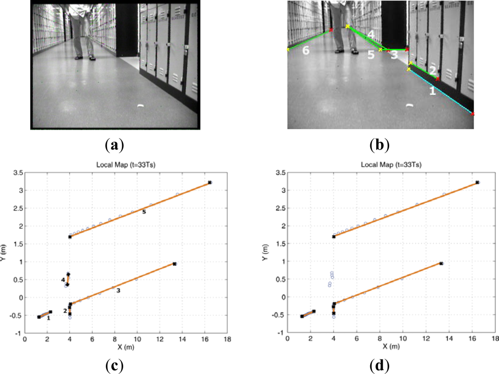
In this experiment, a person stood in front of the robot for few minutes shown in Figure 4(a). The size of ROI defined in Figure 2(a) is u: [0,320] pixel and v: [40,240] pixel. The extracted image lines with the endpoints in this ROI are illustrated in Figure 4(b). Also the segments obtained from laser sensor are displayed in Figure 4(c), and it can be seen that several laser segments, for example laser segment 4, are pseudo features which are related to the dynamic objects. It is clear that these pseudo laser segments can not be removed by the MM-estimate based method proposed in our previous work. To delete these pseudo features, by using the line feature fusion strategy describe in Section 4, we incorporated the image lines with the laser segments and tested all possible hypothesis to determine which laser segment is not the feature.

Table 2. The hypothesis test of feature fusion.

Number of Segments from laser	Number of lines in image
	1	2	3	4	5	6
1	H1	×	×	×	×	×
2	×	×	H1	×	×	×
3	×	×	×	H0	H1	×
4	×	×	×	×	×	×
5	×	×	×	×	×	H1

^×means no fusion process is implemented. H₀ means the laser segments are assumed to assign to the noise, and H₁ implies the laser segments probably are related to image line features.

lists the hypothesis test results. It can be seen that laser segment 4 did not match any image line and it can be eliminated from the set SF_L.

Additionally, it can be found that laser segment 3 correlated with image lines 4 and 5. This is because laser segment 3 concurrently located in the angle interval determined by image lines 4 and 5 respectively. However, it only related to line 5 according to the fusion rule. We applied this feature fusion strategy in the whole EKF laser SLAM process and the result after feature fusion is shown in Figure 5.

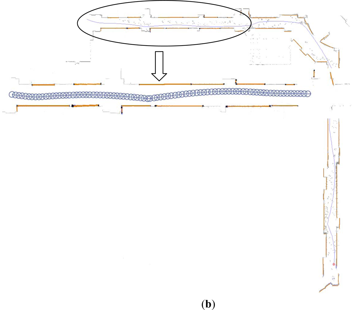
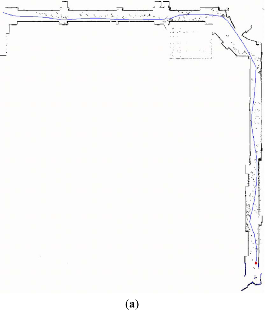
Figure 5(a) is the robot trajectory and grid map plotted by the software of ActivMedia Company with raw laser data. It is obvious that parts of grid map are contaminated by the walking persons. Those raw laser data corresponding to the moving objects lead to the extraction of pseudo laser segments. Fortunately, with the proposed feature fusion method they are almost removed, which is shown in Figure 5(b). And the grid map is overlaid in light gray color for comparison. Furthermore, it can be found in Figure 5(b) that a few of raw laser data related to the static segment features are lost in the final map.

The reasons for this case are: one is the locations of these laser data are out of the HFOV of the camera, the other is the assumptions of proposed Bayesian fusion rule is strict (i.e., pessimistic condition) so that a segment related to the real static object is mis-deleted as the pseudo one. With this experiment, we can state that the feature fusion method is competent for disposing pseudo and confused features.

5.2. Testing the Modified MPEF-SLAM

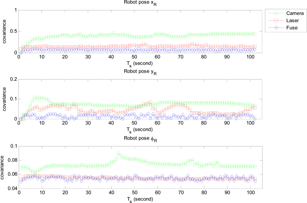
We firstly ran two individual EKF SLAM: monocular SLAM and laser SLAM procedures in parallel mode. The state variable and its covariance obtained respectively from each individual SLAM were integrated to compute the fused state variable and related covariance of the MPEF-SLAM. Finally the fused state variable and covariance were propagated back to monocular and laser SLAM respectively for updating the individual state variables to improve the localization accuracy. Figure 6 illustrates the covariance of the fused and individual robot pose. It can be seen that the covariance of the position: x_R and y_R is obviously reduced after fusion. However, the covariance of the orientation ϕ_R is similar to the value from laser SLAM, but it is more efficient than that from the monocular SLAM. This is because the covariance of the state variable in laser SLAM contributes more for computing the weighted matrix.

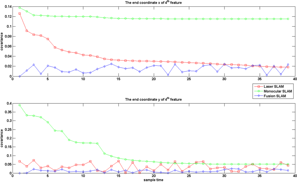
Figure 7 gives the results of covariance on an endpoint of one line feature. We note that the selected line features displayed in Figure 7 for validation are the ones always appearing in 40 consistent images during the experiment. It seems that the covariance of the line endpoints after sensor fusion is also reduced. With these experiments, we may state that the MPEF-SLAM decreases the covariance of state variables and increase the accuracy of localization.

5.3. Testing the HTMDA

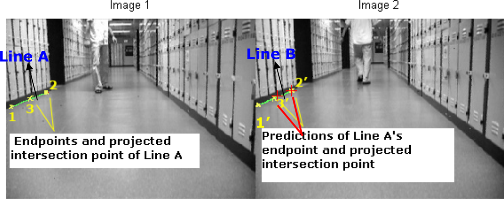
In the defined ROI, we compute M and Σ_M via the current captured image (labeled as image 2 in Figure 8) and one image stored in image sequence buffer, for example the previous image (labeled as image 1 in Figure 8). After that with the estimated M and Σ_M we selected one pair of lines to demonstrate our HTMDA method. As shown in Figure 8, we marked endpoints as 1, 2 and projected intersection point as 3 for Line A of image 1. Those for Line B observed in image 2 are as 1′, 2′ and 3′. According to Equation (5), we obtained the predictions of 2′ and 3′ stressed in red cross in image 2. It can be seen that the prediction of 2′ almost coincides with the 2′, and the prediction of 3′ locates at Line B but is a little bit far from 3′. The position of the prediction of endpoint 1′ is out of the bound of image 2. In this case, we may use condition (7) to decide if Line B is associated with Line A or not, but it is false. Hence the condition in Equation (8-1) has to be considered to test whether the predictions of 1′ and 3′ lie on Line B. Obviously this condition is true. Therefore, we can determine that the observed Line B in the captured image is matched with the Line A stored in the map.

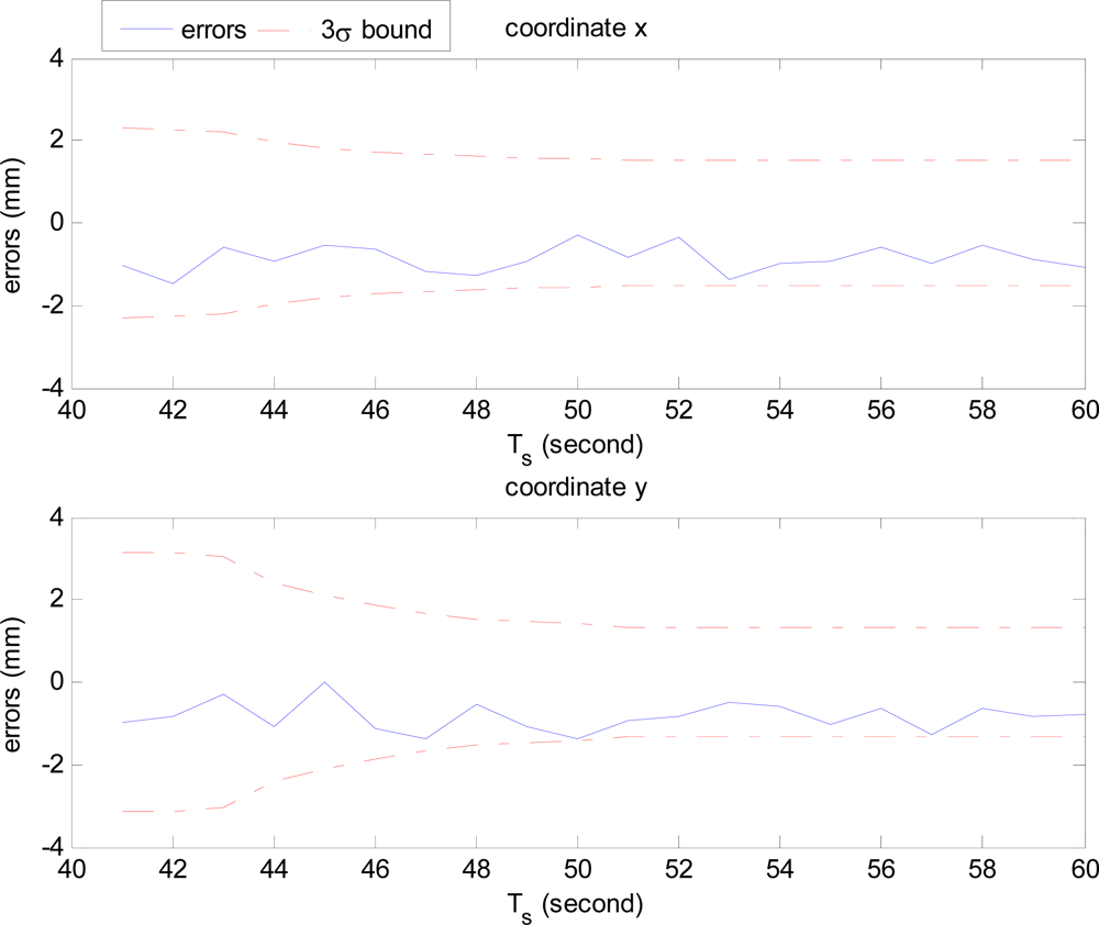
Figure 9 shows the errors of HTMDA for the known endpoint 2 of Line A in Figure 8. Because there is no device in our present experimental conditions for detecting the ground truth of the features, we provisionally measured the truth value by hand as accurate as possible, which follows the process of [31]. Line A appears in around 20 sequential images. As displayed in Figure 9, the actual feature estimation errors are bounded within the 3σ limits, which demonstrates the effectiveness and consistency of the proposed HTMDA.

6. Conclusions

In this paper, we suggest a sensor fusion strategy including feature fusion and modified MPEF-SLAM modules for the SLAM task of autonomous mobile robots in dynamic environments. Our feature fusion policy incorporates the line features extracted by a monocular camera with the segments represented by robust regression model from a laser sensor, the purpose of which is to remove the potential pseudo laser segments corresponding to the moving objects. The modified MPEF-SLAM combines state variable estimates obtained from individual SLAM procedure (monocular and laser SLAM), and respectively propagates the fused state variable backward to each SLAM process to reduce the covariance of the state variable of individual SLAM furthermore improve the accuracy of localization. Additionally, for the data association problem in monocular SLAM we present a new method based on homography transformation matrix. It relaxes redundant computational procedures compared with the algorithm based on pixel by pixel computation. Experimental results verify the performance of the proposed sensor fusion strategy and data association algorithm. The planned future work will include improvement of the feature fusion module on how to use the laser data located outside the HFOV and extension of sensor fusion modules such as sensor management, active sensor. Another promising direction is on developing an online implementation for the proposed HTMDA and MPEF-SLAM algorithm by embedded hardware and technique.

References

- Davison, A.J.; Reid, I.D.; Molton, N.D.; Stasse, O. MonoSLAM: Real-time single camera SLAM. Trans. Pat. Anal. Mach. Intell 2007, 29, 1052–1067. [Google Scholar]
- Strasdat, H.; Montiel, J.M.M.; Davison, A.J. Real-time monocular SLAM: Why filter? Proceedings of the 2010 IEEE International Conference on Robotics and Automation (ICRA), Anchorage, AK, USA, 3–8 May 2010.
- Civera, J.; Davison, A.J.; Montiel, J.M.M. Inverse depth to depth conversion for monocular SLAM. Proceedings of the 2007 IEEE International Conference on Robotics and Automation, Roma, Italy, 10–14 April 2007.
- Eade, E.; Drummond, T. Scalable monocular SLAM. Proceedings of the 2006 IEEE Computer Society Conference on Computer Vision and Pattern Recognition, New York, NY, USA, 17–22 June 2006.
- Montiel, J.M.M.; Civera, J.; Davison, A. Unified inverse depth parametrization for monocular SLAM. Proceedings of the Robotics: Science and Systems 2006, Philadelphia, PA, USA, 16–19 August 2006.
- Eade, E.; Drummond, T. Edge landmarks in monocular SLAM. Proceedings of the 17th British Machine Vision Conference (BMVC), Edinburgh, UK, 4–7 September 2006.
- Gee, A.P.; Mayol-Cuevas, W. Real-time model-based SLAM using line segments. Proceedings of the 2nd International Symposium on Visual Computing, Lake Tahoe, NV, USA, 6–8 November 2006.
- Smith, P.; Reid, I.; Davison, A.J. Real-time monocular SLAM with straight lines. Proceedings of the 17th British Machine Vision Conference (BMVC), Edinburgh, UK, 4–7 September 2006.
- Lemaire, T.; Lacroix, S. Monocular-vision based SLAM using line segments. Proceedings of the 2007 IEEE International Conference on Robotics and Automation, Roma, Italy, 10–14 April 2007.
- Hartley, R.; Zisserman, A. Multiple View Geometry in Computer Vision, 2nd ed; Cambridge University Press: Cambridge, UK, 2003. [Google Scholar]
- Lowe, D.G. Distinctive image features from scale-invariant keypoints. Int. J. Comput. Vis 2004, 60, 91–110. [Google Scholar]
- Zhang, X.; Rad, A.; Wong, Y.-K. A robust regression model for simultaneous localization and mapping in autonomous mobile robot. J. Intell. Robot. Syst 2008, 53, 183–202. [Google Scholar]
- Sola, J.; Vidal-Calleja, T.; Devy, M. Undelayed initialization of line segments in monocular SLAM. Proceedings of the IEEE/RSJ International Conference on Intelligent Robots and Systems (IROS 2009), St. Louis, MO, USA, 11–15 October 2009.
- Folkesson, J.; Jensfelt, P.; Christensen, H.I. Vision SLAM in the measurement subspace. Proceedings of the 2005 IEEE International Conference on Robotics and Automation (ICRA 2005), Barcelona, Spain, 18–22 April 2005.
- Jeong, W.Y.; Lee, K.M. Visual SLAM with line and corner features. Proceedings of the 2006 IEEE/RSJ International Conference on Intelligent Robots and Systems, Beijing, China, 9–15 October 2006.
- Diosi, A.; Kleeman, L. Advanced sonar and laser range finder fusion for simultaneous localization and mapping. Proceedings of the 2004 IEEE/RSJ International Conference on Intelligent Robots and Systems (IROS), Sendai, Japan, 28 September–2 October 2004.
- Zhang, G.; Suh, I.H. Building a partial 3D line-based map using a monocular SLAM. Proceedings of the 2011 IEEE International Conference on Robotics and Automation (ICRA), Shanghai, China, 9–13 May 2011.
- Kaess, M.; Dellaert, F. Covariance recovery from a square root information matrix for data association. Robot. Auton. Syst 2009, 57, 1198–1210. [Google Scholar]
- Margarita, C.; Andrew, J.D. Active matching. Proceedings of the 10th European Conference on Computer Vision: Part I, Marseille, France, 12–18 October 2008.
- Chli, M.; Davison, A.J. Active matching for visual tracking. Robot. Auton. Syst 2009, 57, 1173–1187. [Google Scholar]
- Kaess, M.; Dellaert, F. Probabilistic structure matching for visual SLAM with a multi-camera rig. Comput. Vis. Image Underst 2010, 114, 286–296. [Google Scholar]
- Booij, O.; Zivkovic, Z.; Kröse, B. Efficient data association for view based SLAM using connected dominating sets. Robot. Auton. Syst 2009, 57, 1225–1234. [Google Scholar]
- Kwon, J.; Lee, K.M. Monocular SLAM with locally planar landmarks via geometric Rao-Blackwellized particle filtering on lie groups. Proceedings of the 2010 IEEE Conference on Computer Vision and Pattern Recognition (CVPR), San Francisco, CA, USA, 13–18 June 2010.
- Miro, J.V.; Dissanayake, G.; Weizhen, Z. Vision-based SLAM using natural features in indoor environments. Proceedings of the 2005 International Conference on Intelligent Sensors, Sensor Networks and Information Processing, Melbourne, VIC, Australia, 5–8 December 2005.
- Sim, R.; Elinas, P.; Griffin, M.; Little, J.J. Vision-based SLAM using the Rao-Blackwellised particle filter. Proceedings of the IJCAI Workshop on Reasoning with Uncertainty in Robotics (RUR), Edinburgh, UK, 30 July–5 August 2005.
- Gil, A.; Reinoso, O.; Martinez Mozos, O.; Stachniss, C.; Burgard, W. Improving data association in vision-based SLAM. Proceedings of the 2006 IEEE/RSJ International Conference on Intelligent Robots and Systems, Beijing, China, 9–15 October 2006.
- Gil, A.; Reinoso, O.; Payá, L.; Ballesta, M.; Pedrero, J.M. Managing data association in visual SLAM using SIFT features. Int. J. Fact. Autom. Robot. Soft Comput, 2007, pp. 179–184. Available online: http://arvc.umh.es/documentos/articulos/InternationalSARDataAssociation.pdf (accessed on 16 November 2011). [Google Scholar]
- Ahn, S.; Choi, M.; Choi, J.; Chung, W.K. Data association using visual object recognition for EKF-SLAM in home environment. Proceedings of the 2006 IEEE/RSJ International Conference on Intelligent Robots and Systems, Beijing, China, 9–15 October 2006.
- Chekhlov, D.; Mayol-Cuevas, W.; Calway, A. Appearance based indexing for relocalisation in real-time visual SLAM. Proceedings of the 19th Bristish Machine Vision Conference, Leeds, UK, 1–4 September 2008.
- Zhu, Y. Multisensor Decision and Estimation Fusion; Kluwer Academic Publishers: Boston, MA, USA, 2003. [Google Scholar]
- Wijesoma, W.S.; Perera, L.D.L.; Adams, M.D. Toward multidimensional assignment data association in robot localization and mapping. IEEE Trans. Robot 2006, 22, 350–365. [Google Scholar]
Appendix
The motion models for two SLAM procedures are identical and represented as:
Each individual EKF SLAM is:
For the fused EKF SLAM, there are similar formulas:
According to Equations (19) and (22), can be represented by , i.e.,
Multiplying zk at both side of Equation (21), we have:
Substituting Equation (25) into Equation (24), and then substituting Equations (21) and (24) into Equation (20), we find:
Actually in each iteration, and are constant matrix calculated by the values of and . Therefore and are linear items. With the property of linearity, we may determine:
By Equations (18) and (27), Equation (26) is rewritten as:
It is necessary to note that Equations (23) and (28) manifest the relationship of the state variables as well as the covariance matrix in the fused and individual EKF SLAM. From Equation (28), the weight matrix for each individual state variable can be determined. That is:
If the latest fused state estimate is broadcasted to every individual state estimate as the back propagation (named feedback), we can prove that the covariance of state variable is reduced with this feedback but the performance of the fused EKF SLAM is unchanged with and without the feedback.
To maintain the identity with [30], we apply the same symbols and assumptions, and the general symbols x̂ and P̂ mean the state variable and its covariance when the feedback is considered. Concerning the feedback, the individual and fused one-step predictions are:
Rewriting Equations (23) and (28) by using Equation (30) as:
Suppose that the initial values of state variable vector and covariance for fused and individual EKF SLAM are same, i.e.,
At step k, substituting Equation (34) into Equation (31), we have:
Similar to Equation (19), we can get:
Substituting Equation (36) into Equation (35), we obtain:
In comparing with Equation (23), we claim that :
On the other hand, with assumptions above we get the following equations by substituting Equation (18) into Equation (15):
With replacement of the related item in Equation (32) by Equation (39), and considering the conditions of Equation (34), the following derivation is obtained:
Comparing Equations (40) and (41), we assert that:
It is obvious from Equations (38) and (42) that the performance of fused EKF SLAM does not change in the presence or absence of feedback. However, when the feedback is allowed into the individual EKF SLAM, the fused covariance of the state variable is decreased. This result is verified as follows: by Equations (19) and (37) we have the equation:
It is easy to prove that Equation (43) is equal and larger than zero because (cf. [30]). Therefore, we have , that is:
It can be concluded that Equations (44) and (45) suggest that under a certain constraint the fused covariance of the state variable is reduced with the feedback. And when we use this fused state variables in SLAM, it will reduce the error of the localization and map features without changing the performance of individual EKF SLAM.