Atmospheric pollution is a problem as global warming is caused by the man-made addition of extra amounts of greenhouse gases such as CO₂, N₂O and CH₄. Current average mixing ratios of the trace components CO₂, N₂O and CH₄ in the atmosphere are ∼380, ∼1.8 and ∼0.32 parts per million by volume (ppmv), respectively. CO₂ is released into the atmosphere when fossil fuels, coal, solid waste and wood products are burned, during cement production, and also when land surface cover is changed by humans. Increased CH₄ levels come from fossil fuels, rice cultivation, animal husbandry, biomass burning and landfills. The main anthropogenic sources of N₂O are agriculture, and industrial sources including adipic and nitric acid production. Combustion of solid waste and fossil fuels also contributes to atmospheric N₂O. The need to detect these trace gases has become increasingly important in recent years, both for controlling industrial processes and for monitoring air quality. Since many trace gases have a significant impact on the environment, the development of techniques for its fast, accurate and sensitive detection is required [1–5].

Laser based spectroscopy provides interesting advantages related to its high selectivity and sensitivity in the detection of trace gases. Semiconductor diode lasers emitted the near infrared (NIR) light have played a central role, being tunable spectroscopic light sources which exhibit a relatively low amplitude noise [6]. In addition, their small size and the relatively low cost have made them particularly suitable for the realization of transportable spectrometers employed for in-situ measurements [7,8]. In the NIR region, relatively weak overtone or combination vibrational transitions occur for trace gases relevant to the atmospheric environment. Although line strengths of these transitions are a few orders of magnitude lower than transitions belonging to fundamental vibrational bands, cavity ring down spectroscopy (CRDS) [9] and frequency modulation spectroscopy (FMS) with a single-mode diode laser in the near infrared region have allowed to achieve the detection of low concentrations (< sub ppmv) of trace gases [10]. The use of multi-pass absorption cells [11] further improves the sensitivity, since the effective optical path is increased up to several tens or hundreds of meters. Phase-sensitive techniques, which are the core of the FM techniques, significantly reduces the 1/f electronic noise, achieving high detection sensitivity. In most cases the detection sensitivity is only limited by noise introduced by undesired optical fringes and drifting of laser power and detector sensitivity. Wavelength modulation spectroscopy (WMS) [12–16] is a kind of FMS with a modulation frequency lower than the spectral line width of interest. In the case of WMS, the lower modulation frequency allows one to use low-frequency circuits and photo detectors, reducing the complexity and the cost of measurement system. Recently, a high sensitive open path CH₄ analyzer based on WMS detection and Herriott cell design with a 30 m total optical path length has been developed which is commercially available [17].

In the present study, we demonstrate the detection of greenhouse gases such as CO₂, CH₄ and N₂O using WMS. The aim of this work is characterized the optimum condition of the detection of greenhouse gases by NIR-WMS. The optimum pressure for the detection of CO₂, N₂O and CH₄ by WMS is investigated both experimentally and theoretically by taking into consideration background noise in the WMS.

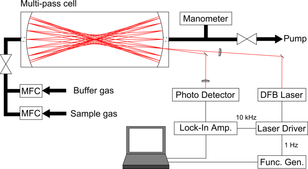
We used WMS in the near-infrared region for trace gas detection. Figure 1 shows a scheme of our experimental apparatus. All optical elements were properly designed to reduce their dimensions and mechanical instability as much as possible. Three distributed feed-back (DFB) diode lasers (NTT Electronics) with a tuning range of ± 1 nm were used as light sources. The first DFB laser with a center wavelength of 1,572 nm was used to detect CO₂ at the 3ν₁ + ν₃ combination band. The second DFB laser with a center wavelength of 1,515 nm was used to detect the N₂O line at the 3ν₃ overtone band. The last DFB laser with a center wavelength of 1,651 nm was used to detect CH₄ at the 2ν₃ overtone band. The laser power varied as a function of injection current with a maximum of 20 mW. The wavelengths of these DFB lasers were chosen for strong absorbing transitions and no interference of water.

The laser wavelengths were tuned by varying the laser temperatures, while fine tuning was accomplished by changing the laser diode injection currents. To minimize fringe noise from optics, anti-reflection (AR) coated lenses and AR coated and wedged windows were used. The output beam was focused by an AR coated lens (f = 50 cm) to the centre of a Herriott-type multi-pass cell [11] with a distance of 40.4 cm between two mirrors. In the multi-pass cell, the laser beam undergoes multiple reflections between two mirrors; the total number of 74 passes corresponds to the optical path length of 29.91 m. The inner volume of the cell is 900 cm³. The beam passed through the multi-pass cell was finally focused by a short focal AR coated lens (f = 5 cm) onto an InGaAs photodiode detector (Hamamatsu G5852-11).

The laser wavelength was sinusoidally modulated at 10 kHz, and scanned at 1 Hz around the absorption line. The laser wavelength scan and modulation were performed through a custom-made laser driver. The background bias signal of the laser driver used in this study was same level as that of a commercial driver (e.g., ILX LDC3724C). Under typical conditions, the modulated absorption signal was phase-sensitive detection at twice the modulation frequency (2f) using a lock-in amplifier (Stanford Research System SR810 DSP) with the time constant set to 3 ms. The data was acquired via a 16 bit AD PCMCIA card (CONTEC ADA16-8/2(CB)L) to a laptop computer and analyzed using software written in LabVIEW.

N₂ (99.99%) and premixed gases of synthesized air (79% N₂, 21% O₂), 1% CO₂ in N₂, 1% N₂O in N₂, and 0.1% CH₄ in air were purchased from Taiyo Nippon Sanso Co. The flow rate of the feed was controlled with mass flow controllers (Kofloc MODEL3660). The total pressure was monitored with a capacitance manometer (Setra Systems MODEL720). All measurements were performed at room temperature (293 ± 3 K).

The general theory of the FMS and WMS has been well summarized in the works of previous researchers [13–15]. In the case of sinusoidal modulation with modulation index β and frequency ω_m, the optical field E with carrier frequency ω₀ is given by: (1) E ( t ) = E 0   exp [ i ( ω 0 t + β   sin   ω m t ) ] = E 0   exp ( i ω 0 t ) ∑ n = − ∞ + ∞ J n ( β ) exp ( in   ω m t )where the expansion in a series of nth-order Bessel functions J_n characterizes the frequency components of the modulated light spectrum. FMS is classified by its modulation frequency ω_m. WMS uses ω_m that is much less than the spectral line width Γ of the absorption line of interest. Conversely, narrowly-defined FMS uses ω_m ≫ Γ. In the case of WMS, the probe beam modulation is generally treated as instantaneous frequency change: (2) ω i ( t ) ≡ d d t ( ω 0 t + β   sin   ω m t ) = ω 0 + Δ F   cos   ω m twhere the maximum frequency deviation from the carrier frequency ω₀ is ΔF = βω_m. In this model, dispersion effects cannot be considered, and the light intensity transmitted through the sample is expressed by I_T = I₀ exp(−α), where α is the absorption coefficient.

On the assumption that α(ω) ≪ 1, I_T(ω) ≈ I₀(ω)[1 − α(ω)], the α(ω) can be expanded into the Taylor series around the carrier frequency ω₀: (3) I T ( ω ) = I 0 ⌊ 1 − a ( ω 0 ) − d α d ω | ω 0 ( ω − ω 0 ) − 1 2 ! d 2 α d ω 2 | ω 0 ( ω − ω 0 ) 2 − 1 3 ! d 3 α d ω 3 | ω 0 ( ω − ω 0 ) 3 − … ] = I 0 ⌊ 1 − a ( ω 0 ) − d α d ω | ω 0 Δ F   cos ⁡   ω m t − 1 2 ! d 2 α d ω 2 | ω 0 ( Δ F ) 2 1 2 ( 1 +   cos ⁡   2 ω m t ) − 1 3 ! d 3 α d ω 3 | ω 0 ( Δ F ) 3 1 4 ( 3   cos ⁡   ω m t +   cos ⁡   3 ω m t ) … ] .

Here cos² ω_mt, cos³ ω_mt, etc., have been expanded with trigonometric identities for convenience in picking off the power at any frequency of interest. Because the instantaneous frequency varies sinusoidally, the Taylor series of I_T(ω) is more or less automatically the Fourier series, too. This series will not converge well for some ΔF [16]. However, if the frequency deviation ΔF is sufficiently small compared with Γ, higher-order terms can be neglected, and the WMS signal that is coherently detected at the frequency nω_m is proportional to the n-th derivative of the sample absorption.

In the present study, the assumption that ΔF ≪ Γ was not valid under some experimental conditions. Thus we used the frequency domain approach to calculate the WMS spectral line shape. In the real system, the DFB laser intensity is not uniform over the FM range, and simultaneous amplitude modulation (AM) of the electric field occurs such that: (4) E ( t ) = E 0 [ 1 + M   sin   ( ω m t + ψ ) ] exp [ i ω 0 t + i β   sin   ( ω m t ) ]where M and ψ denote the AM index and the phase difference between AM and FM. By expanding the AM term in term of exponentials, i.e., Msin(ω_mt + ψ) = M/2[exp{i(ω_mt + ψ)} − exp{i(ω_mt + ψ)}], and replacing the exponential frequency terms as a summation over Bessel functions, one can rewrite Equation (4) as: (5) E ( t ) = E 0   exp ( i ω 0 t ) ∑ n = − ∞ ∞ r n   exp ( in   ω m t )where: (6) r n = ∑ k = − 1 1 a k J n − k ( β ) ,                     a 0 = 1 , a ± 1 = ± M 2 i exp ( ± i ψ )Equation (1) is the special case of Equation (5) where M = 0.

When the modulated electric field E(t) is passed through a medium exhibiting the field amplitude attenuation δ(ω) and the optical phase shift φ(ω), the transmitted optical field is then: (7) E T ( t ) = E 0   exp ( i ω 0 t ) ∑ n = − ∞ ∞ exp ( − δ n − i φ n ) r n   exp ( in   ω m t )where δ_n = δ(ω₀ + nω_m) and φ_n = φ(ω₀ + nω_m). Because the intensity I equals cɛ₀EE*/2 in SI units, the absorption coefficient α is twice the electric field amplitude attenuation coefficient δ for weak absorption. The transmitted intensity can be expressed as a sum of Fourier components at frequencies corresponding to multiples of ω_m [13]. In the case of 2ω_m detection, the resulting signal is: (8) I = 2 I 0 [ Re ( Z ) cos   θ − Im ( Z ) sin   θ ] ,                 Z = ∑ n = − ∞ ∞ r n + 1 r n − 1 * [ exp ( − ( δ n + 1 + δ n − 1 ) ) + i ( φ n + 1 − φ n − 1 ) ]where θ refers to the phase difference between the transmitted intensity and the reference signal in the lock-in amplifier. The in-phase (0 or π) component corresponds to absorption, and the quadrature (±π/2) components correspond to dispersion of the incident light. In the absence of absorption and dispersion, Z has a nonzero value due to residual amplitude modulation (RAM) [14]. In the case of 2ω_m detection, the background bias signal is: (9) I RAM = 1 2 M 2 I 0   cos ( θ + 2 ψ + π )

Since I_RAM linearly depends on I₀, low frequency noise in I₀, such as fringe noise from optics and drifting of laser power and detector sensitivity, within the noise equivalent bandwidth of the lock-in amplifier is converted into FM/WM signal background noise.

WM spectra are calculated from Equation (8) assuming that the absorption peak shape is described by the Voigt function. The Voigt function was calculated following the algorithm described by Humlicek [18] and Schreier [19]. The Doppler half width at half maximum (HWHM) was calculated from the temperature and molecular weight. To calculate homogeneous HWHM values, the pressure broadening factor was taken from the HITRAN database [20]. The FM index β was estimated from β = ΔF/ω_m. To calculate the AM index M, the intensity dependence on the laser frequency was measured, separate from the WMS experiments. Table 1 shows the parameters used in the spectral simulation. For the modulation frequency below 750 MHz, the AM-FM phase difference ψ has been found to have a value of ca. nπ + π/2 [14]. For the present study, negative dependence of the laser intensity on the laser frequency suggests that ψ ≈ −π/2. In the WMS condition, i.e., ω_m ≪ Γ, the dispersion term is negligibly smaller than the absorption term, thus the detection phase θ ≈ 0 for the maximum signal intensity. 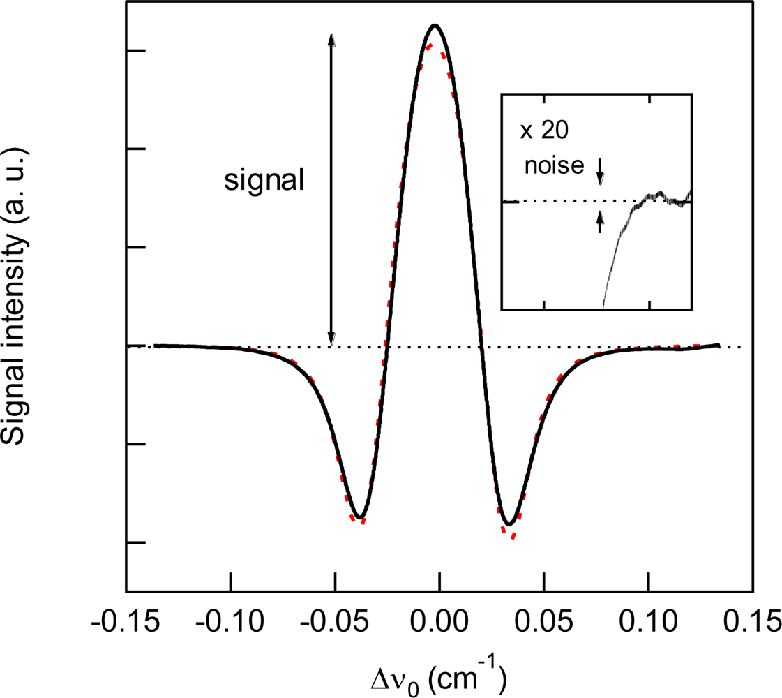In all calculations, the values of ψ and θ were fixed to be –π/2 and 0, respectively. 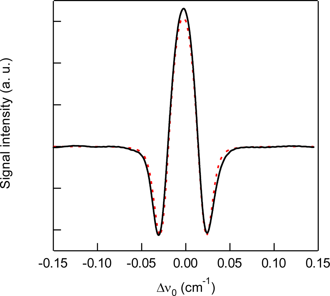The signal intensity and noise are defined as peak-to-baseline amplitude and peak-to-peak variation of 2f signal with standard deviation of baseline, as shown in Figure 2.

For the detection of CO₂, we used the 3ν₁ + ν₃ combination band of the R(16) line at the absorption line center of 6,359.97 cm⁻¹, which is free from interference by the other atmospheric species and has a line strength of 1.73 × 10⁻²³ cm² molecule⁻¹ cm⁻¹, according to the HITRAN database [20]. Figure 2 shows experimental and simulated spectra of 1% CO₂ at a total pressure of 15 kPa, diluted by N₂. The experimental spectra were acquired with a lock-in time constant of 3 ms and filter slope of 24 dB/oct, which leads a noise equivalent bandwidth of the low pass filter to be 26 Hz. The simulated spectrum reconstructed the experimental spectrum well. 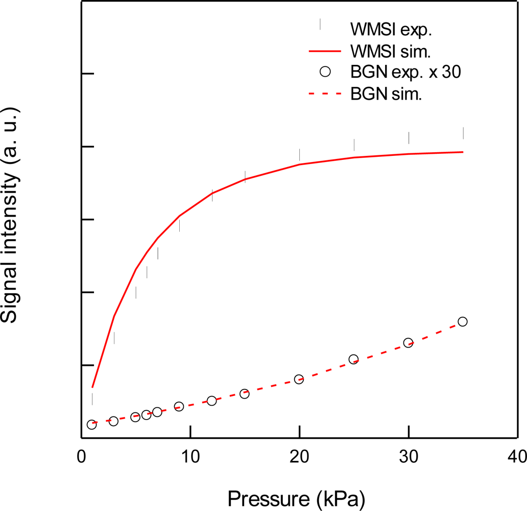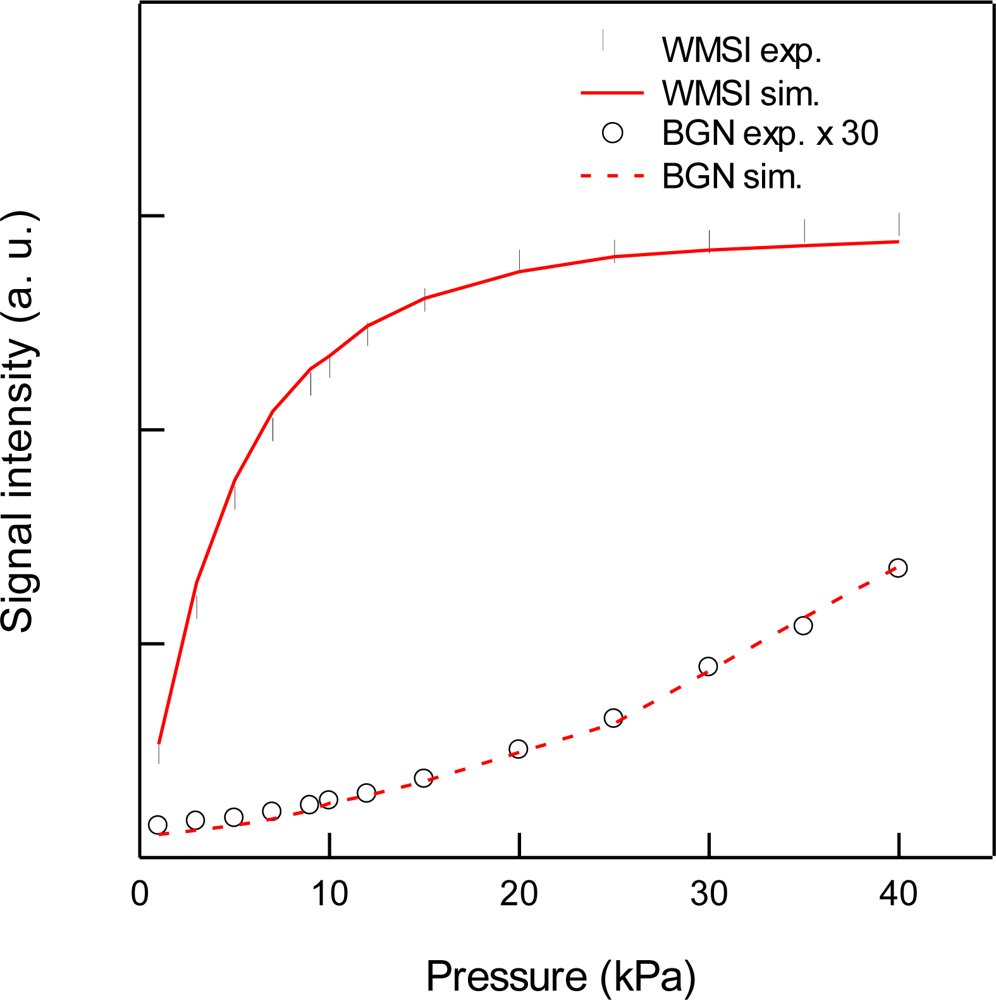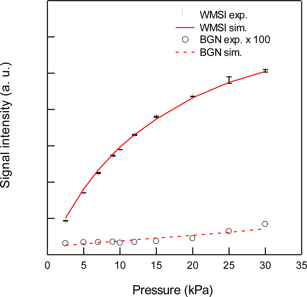Figure 3 shows the total pressure dependence of signal intensity and background noise. In all experiments, the modulation depth ΔF were adjusted to obtain the maximum signal intensity. The concentration of CO₂ was maintained at 1% in N₂. In the simulation, we assumed that background noise was linearly dependent on M², according Equation (9), and the simulated noise intensities were normalized to minimize the residual to experimental values. As can be seen, the simulated results closely agree with the experimental measurements. The signal intensity profile of Figure 3 shows two opposing effects of pressure: decreasing spectral line centre intensities due to pressure broadening and an increasing absorber number density with increasing pressure. At low pressures (Doppler regime), the signal intensity increases linearly with pressure, while at high pressures (Lorentzian regime) the signal intensity become almost constant due to the canceling of two opposing terms with pressure. 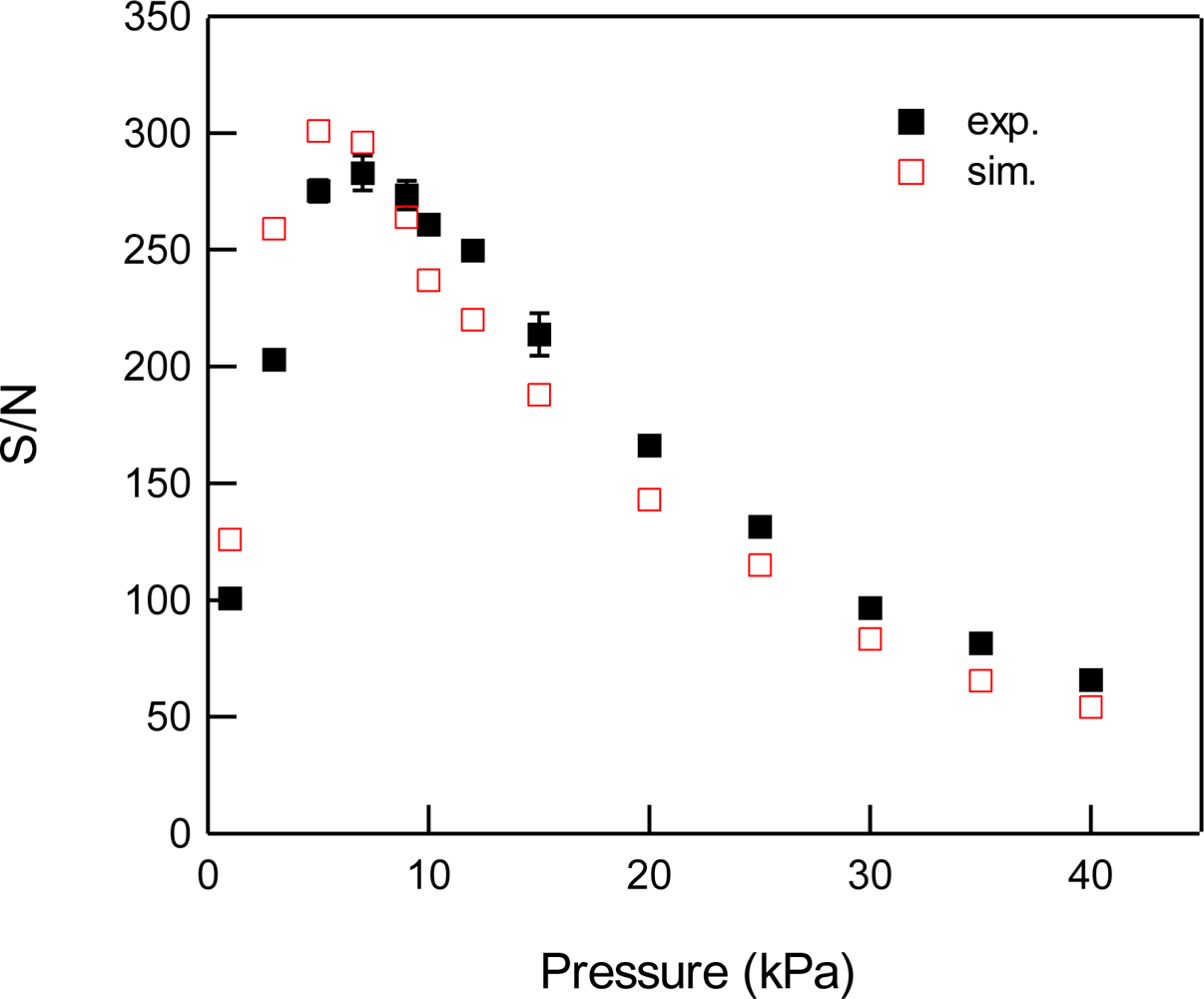Figure 4 shows experimental and simulated profiles of the signal to noise ratio (S/N) as a function of total pressure. The optimum total pressure in the detection of CO₂ was found to be around 7 kPa. In the WMS, optimization of the signal intensity occurs at ΔF/HWHM = 2.2 in the Voigt function to calculate the properties of the 2f line shape [21].

Because the Voigt HWHM is increased by pressure broadening with increasing pressure, the frequency deviation ΔF must be increased in order to maximize the WMS signal with increasing pressure. Since the AM index M depends linearly on ΔF, i.e., M/ω_mβ (= M/ΔF) is constant, and the residual amplitude modulation I_RAM is linearly dependent on M² according to Equation (9), the low frequency noise in I₀ such as the fringe noise from optics and drifting of laser power and detector sensitivity was enlarged by factor of M² at higher pressure, as shown in Figure 3.

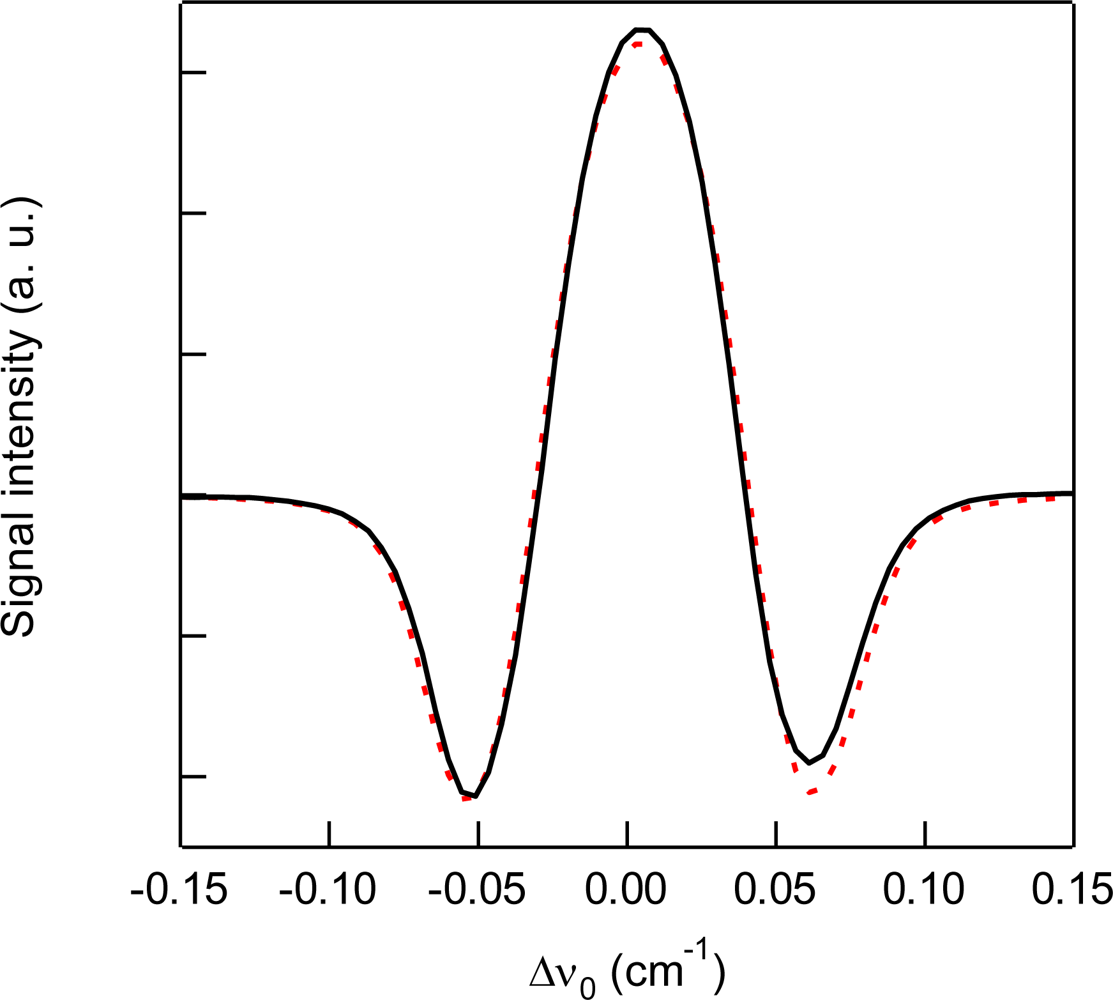
In the case of N₂O detection, the 3ν₃ overtone band of the R(15) absorption line at 6,591.44 cm⁻¹ with a line strength of 2.33 × 10⁻²³ cm² molecule⁻¹ cm⁻¹ was monitored. Figure 5 shows the experimental and simulated spectra of 1% N₂O at a total pressure of 6 kPa. As for the previous experiment of CO₂, the acquired 2f WM spectrum of N₂O shown in Figure 5 is in excellent agreement with the simulated spectrum. Figure 6 shows the total pressure dependence of signal intensity and background noise for the 1 % N₂O diluted in N₂. The signal intensity is saturated above 20 kPa. Figure 7 shows experimental and simulated profiles of S/N as a function of total pressure. The simulated results agreed with the experimental results. The optimum total pressure for the detection of N₂O is estimated to be around 6 kPa.

For the detection of CH₄, we used the R(3) lines of the 2ν₃ overtone band around 6,046.95 cm⁻¹ with a line strength of the order 10⁻²¹ cm² molecule⁻¹ cm⁻¹ [20]. As listed in Table 2, there are three absorption peaks at around 6,046.95 cm⁻¹. Figure 8 shows the experimental and simulated spectra of 0.01% CH₄ at around 6,046.95 cm⁻¹ and total pressure of 10 kPa. The three absorption lines were considered in the simulation. In the experimental spectra, only one absorption peak was observed at 6,046.95 cm⁻¹ due to the overlapping of the three absorptions. Figure 9 shows the total pressure dependence of signal intensity and noise for the 0.01 % CH₄ diluted in N₂. 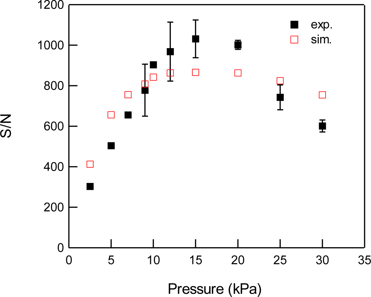Figure 10 shows the experimental and simulated profiles of S/N as a function of total pressure. The simulated spectrum using the three absorption lines reproduces the experimental results well. The optimum total pressure of CH₄ detection at the 6,046.95 cm⁻¹ absorption peak was found to be around 15 kPa. The larger optimum pressure for CH₄ detection compared with those for CO₂ and N₂O would be caused by the broader nature of the absorption peak consisting of three closely separated absorption lines.

To estimate the limit of detection (LOD) of the present system, we changed the mixing ratio of sample gases, while keeping the optimum value of the total pressure fixed. The measurements were performed with a noise equivalent bandwidth of 26 Hz. From a fit of the signal intensity as a function of CO₂ mixing ratio at 7 kPa, we found, for a signal to noise ratio of 2, the LOD of [CO₂]^7kPa = 24 ± 2 ppmv. In the case of N₂O, the LOD at 6 kPa was estimated to be 7.6 ± 0.4 ppmv. For CH₄, we estimated the detection limit and NEAS using the R(3) peaks at 15 kPa to be 60 ± 4 ppbv. The LODs for the three gases had an almost linear dependence on the absorption cross sections. The line strengths of CO₂, N₂O and CH₄ of the used transitions vary slightly with temperature (0.23, 0.25 and 0.39%, respectively, by temperature change of 1 K around room temperature), however, the LODs are unaffected by temperature change. Parkes et al. demonstrated the detection of N₂O by diode laser cavity ring-down spectroscopy using the same 3ν₃ overtone band [22]. The limiting sensitivity was 23 ppmv at 1 atm with mirror reflectivities of R = 0.9998, which is comparable with our 2f WMS value of 7.6 ppmv. The noise-equivalent absorption sensitivity (NEAS) per scan for a signal to noise ratio of 1 was estimated using following Equation (10): (10) NEAS = Abs min l   NEBW / Nwhere Abs_min, l, NEBW and N denote the absorbance at S/N = 1, the effective optical length of 29.91 m, the noise equivalent bandwidth of 26 Hz and the average number of 20 times, respectively. In the calculation of Abs_min, the absorption line shapes were assumed to be described as the Voigt functions. The estimated values of NEAS for CO₂, N₂O and CH₄ were found to be (1.3 ± 0.1) × 10⁻⁸, (4.8 ± 0.3) × 10⁻⁹, and (5.6 ± 0.4) × 10⁻⁹ cm⁻¹ Hz^−1/2, respectively. The higher value of NEAS for CO₂ would be caused by the larger value of M/ω_mβ, as shown in Table 1, which results the larger effect of the residual amplitude modulation.

We have described the highly sensitive detection of CO₂, N₂O and CH₄ by 2f WMS, using tunable near-infrared diode lasers in the near-infrared region. The observed 2f WM spectra were analyzed as a function of the total pressure. At the optimum total pressure for the detection of each gas, as determined by experimental and theoretical approaches, the limits of detection in the present system were determined. Detection of atmospheric N₂O (320 ppbv) at the 3ν₃ overtone band is not sufficient with our current WMS spectrometer. However, the necessary sensitivity could be delivered by reducing the optical fringe noise and the drifting of laser power using external modulators instead of direct laser modulation.