Do Different Teams Produce Different Results in Long-Term Lichen Biomonitoring?

Abstract

Lichen biomonitoring programs focus on temporal variations in epiphytic lichen communities in relation to the effects of atmospheric pollution. As repeated surveys are planned at medium to long term intervals, the alternation of different operators is often possible. This involves the need to consider the effect of non-sampling errors (e.g., observer errors). Here we relate the trends of lichen communities in repeated surveys with the contribution of different teams of specialists involved in sampling. For this reason, lichen diversity data collected in Italy within several ongoing biomonitoring programs have been considered. The variations of components of gamma diversity between the surveys have been related to the composition of the teams of operators. As a major result, the composition of the teams significantly affected data comparability: Similarity (S), Species Replacement (R), and Richness Difference (D) showed significant differences between “same” and “partially” versus “different” teams, with characteristics trends over time. The results suggest a more careful interpretation of temporal variations in biomonitoring studies.

1. Introduction

Given their strict dependence on the atmosphere for water and mineral supply [1], lichens are extremely sensitive to substances that alter the atmospheric composition. Their occurrence is therefore modulated by pollution levels, thus justifying their wide use as bioindicators of air pollution [2]. Among other biomonitoring methods, the Lichen Diversity Value (LDV) grounds on the assessment of any change in the frequency and abundance of all epiphytic lichen species [3,4,5]. Though it was originally developed for investigating the effects of phytotoxic gases, such as SO₂ and NO_x [5,6,7,8], methods based on the assessment of lichen diversity have also been extensively applied for detecting the sustainability of forest management [9,10,11,12,13], estimating the impact of disturbances related to land use change [14,15,16], and monitoring local- and large-scale effects of climate change [17,18,19,20,21].

Although the disturbances reported above have different drivers, they all cause changes in the diversity, abundance, and composition of epiphytic lichen communities. As lichens are slow-growing organisms, they can be used as long-term biomonitors and the potential trends of the biological effects caused by environmental changes can be monitored by repeated measures over time [22,23]. The extent, and spatial and temporal range of these changes are related to the level and type of impact produced, considering environmental background. Regardless of the cause, the changes can be assessed by monitoring variations in lichen communities in subsequent samplings, taking into account the situation observed at a reference time. Although these changes are classically measured in terms of diversity and abundance (e.g., Lichen Diversity Value—LDV [5]), recent works have shown that variations can also be described by components of the gamma diversity, such as species replacement, richness difference, and similarity [24,25].

The temporal trend of the diversity of the epiphytic lichen communities is however determined by various factors that can interact in an additive or multiplicative way, often making a robust interpretation of the observed data difficult [26]. Among them: (1) changes induced by the temporal variation of the disturbing factors that affect the study area (e.g., increase or decrease in atmospheric pollution) [2]; (2) changes in composition and specific abundance due to the natural succession of the communities [27]; (3) apparent variations in the diversity due to sampling errors [22,26,28] (i.e., due to the fact that in subsequent surveys the same sampling units and / or the same trees are not always detected); (4) changes in perceived diversity due to non-sampling errors, including the operator effect (i.e., due to the fact that, under the same conditions, different people can identify different species or even overlook some lichen species) [29].

Normally the first factor of variation (effects caused by disturbances) is the target of biomonitoring studies, while natural succession is often intrinsically taken into account by the assumption that natural variations can develop randomly throughout a study area. As far as the sampling error is concerned, it is often minimized by the maintenance of the same sampling units in long term studies [6].

The operator effect (non-sampling error) has been tackled in numerous studies that have tried to evaluate it on the basis of intercalibration tests between individual operators or groups of operators [29,30,31,32,33]. These tests represent basic activities for the assessment of quality assurance [34]. As lichen biomonitoring is based on the identification of all epiphytic lichen species within a sampling grid, it requires very high levels of taxonomic knowledge [6,29,30,31,32,35,36]. In this regard, it has been shown that the effect of the operator can sometimes be relevant, even when expert lichenologists are involved in the sampling procedure. For example, during an intercalibration ring test conducted in Italy, only a small number of skilled operators reached the Measurement Quality Objective (MQO) for accuracy of taxonomic identification [29]. Consequently, the periodic and frequent comparison between operators through intercalibration procedures is a fundamental step to guarantee the quality and comparability of the data collected in different areas or in the context of repetitive surveys in the same area. European guidelines for assessing lichen diversity [3] take into account Quality Assurance procedures and field checks on data reproducibility, establishing that the personnel involved in biomonitoring studies must fulfill high levels of taxonomic accuracy and precision to guarantee the reliability and consistency of data collected by different teams.

Data reproducibility is crucial, especially in the case of large-scale, mid-term, or long-term biomonitoring programs or when a before–after approach is foreseen. In fact, in both cases the repetitions of field surveys over time are supposed to be or may be conducted by different teams of specialists.

This is a current topic because in recent years biomonitoring results have been used in the context of environmental forensics [37,38]. Even more so, it is fundamental to provide robust and defensible data, and quality assurance procedures related to the control and evaluation of non-sampling errors play a major role.

Despite several studies on intercalibration between operators having been conducted, no one has yet evaluated the effect of the taxonomic expertise of a team on real data of repeated biomonitoring surveys.

In this paper, we analyzed lichen diversity data collected in Italy from 2007 to 2016 within several ongoing biomonitoring programs. We aimed to study the temporal variations of lichen diversity between repeated investigations in relation to the team composition, distinguishing between surveys carried out by the same or by different teams. By providing information on the variability associated with the operator effect, the results of our work can contribute to improving the interpretative framework of biomonitoring data.

2. Materials and Methods

2.1. Survey Selection and Sampling Design

We analyzed lichen diversity data collected in Italy from 2007 to 2016 within six ongoing biomonitoring programs (

Table 1. Descriptive statistics of the biomonitoring surveys considered within the six study areas. Average Similarity (S), Species Replacement (R), and Richness Difference (D) at tree level for each pair of surveys in the same area are reported, together with the total number of species found.

Study Area	N Trees	N Plots	Gamma Diversity (N Species)	Survey Pair (Years of Surveys)	Team Composition in the Surveys	Delta Years	Av. Similarity (S)	Av. Richness Difference (D)	Av. Species Replacement (R)
A	78	26	84	2008 versus 2009	same	1	72	12	15
				2008 versus 2011	partially	3	52	20	28
				2008 versus 2012	partially	4	48	22	30
				2008 versus 2014	partially	6	47	23	31
				2008 versus 2015	different	7	46	20	34
				2009 versus 2011	partially	2	63	17	20
				2009 versus 2012	partially	3	56	19	25
				2009 versus 2014	partially	5	53	18	29
				2009 versus 2015	different	6	52	20	28
				2011 versus 2012	same	1	74	11	15
				2011 versus 2014	same	2	64	14	22
				2011 versus 2015	partially	3	61	18	21
				2012 versus 2014	same	2	69	15	17
				2012 versus 2015	partially	3	65	18	17
				2014 versus 2015	partially	1	82	12	6
B	108	36	119	2007 versus 2009	different	2	72	11	17
				2007 versus 2012	same	5	62	14	24
				2007 versus 2015	different	8	49	18	34
				2009 versus 2012	different	3	70	11	19
				2009 versus 2015	different	6	54	15	30
				2012 versus 2015	different	3	55	16	29
C	135	39	55	2012 versus 2016	partially	4	58	25	17
D	73	21	98	2010 versus 2013	different	3	57	21	22
				2010 versus 2016	same	6	62	14	24
				2013 versus 2016	different	3	53	18	30
E	71	24	83	2009 versus 2012	same	3	71	13	15
F	135	42	94	2014 versus 2016	partially	2	81	9	10

). The study areas are located all over Italy, from the dry Mediterranean to the humid sub-Mediterranean phytoclimatic belts. The landscape is generally hilly, with elevation ranging from 0 to 800 m. All sites are characterized by urban, industrial, agricultural, and forest areas, within Mediterranean oak vegetation. On average, lichen gamma diversity among the study areas was similar (Table 1), although the range of variation within each study area was considerable. Lichen diversity has been sampled only on trees with similar bark characteristics (sub-acid bark, Quercus and Tilia). For the purpose of this study, we define “biomonitoring program” as a set of lichen biomonitoring surveys repeated in the same study area over time. For every single program, all possible comparisons between subsequent biomonitoring surveys carried out at different times were considered (from here on we refer to these as “survey pairs”). Overall, the time elapsed between repeated surveys ranged from a minimum of 1 to a maximum of 8 years. Biomonitoring programs were always carried out by teams of two skilled and qualified lichenologists. In particular, all operators had an extensive experience in lichen taxonomy and lichen biomonitoring (from a minimum of 15 to a maximum of 25 years of experience). They all have been qualified by specialist training courses where they have reached the requested quality objectives. However, the team composition was not always constant over time; in some cases the study repetition was conducted by the same two operators (subsequently we will refer to this category of team as “same”), in other cases by two different operators (subsequently called “different”), and in a third case only one of the two operators took part in both investigations (subsequently called “partially”).

Conforming to the standards described by Asta et al. [5] and the Italian guidelines [4], plots were selected by systematic sampling, and 3 to 12 trees were selected within each plot. Epiphytic lichen diversity was sampled on trees belonging to species with sub-acid bark (Quercus spp. and Tilia spp.) and with the following characteristics; tree circumference > 60 cm; bole inclination <10°; absence of damage and decorticated areas on the trunk and moss cover <25% of the observation grid. The abundance of each lichen species was sampled on the bole of each tree. For each sampled tree, the Lichen Diversity Value (LDV) was obtained by the sum of the abundance of all lichen species occurring within a 10 × 50 cm observation grid, divided into 5 squares of 10 × 10 cm, placed at each of the four cardinal points of the trunk (N, S, E, W) at a height of 100 cm above the ground. In the repeated surveys within each biomonitoring program, the teams always sampled the same individual trees in the same plots.

2.2. Data Analysis

For each survey pair, we analyzed pairwise comparisons between lichen communities sampled on the same trees. The species presence/absence data matrix was analyzed with SDR Simplex software using the Simplex method—SDR Simplex (Similarity, richness Difference, species Replacement) [39]. For all pairs of the same trees sampled in different surveys, we evaluated the relative contributions of the components of gamma diversity, i.e., Similarity, S; Richness Difference, D; and Species Replacement, R.

Particularly, S corresponds to the Jaccard coefficient of similarity:

S = (a/n) × 100,

(1)

where a is the number of species shared by two surveys and n is the total number of species.

D was calculated as the ratio of the absolute difference between the species numbers of each tree (b, c) and the total number of species, n:

D = (|b − c|/n) × 100,

(2)

R was calculated as:

R = (2 min {b,c}/n) × 100

(3)

Generalized Linear Mixed Models (GLMM) were applied for analyzing the relationships between R, D, and S and predictor variables. In particular, we took into account the effects on gamma diversity components of the following predictors: (1) composition of the teams (“same”, “partially” and “different”); (2) Lichen Diversity Value sampled in the first survey of each program (“LDV at T₀”; (3) time elapsed between survey pairs of the same programs (“delta years”). Plot ID, nested within the Study area, was considered as random effect. A Gaussian error distribution and an identity link function were considered for the models. The Akaike Information Criterion (AIC) [40] was calculated for each model, using the lme4 package [41] in R version 3.5.2 [42].

To analyze the taxonomic agreement between subsequent samplings, for each species in each survey pair the percentage agreement was calculated as follows:

% Agreement = (CP/(CP + SR)) × 100,

(4)

where CP (co-presence) is the number of trees on which the species was found in both surveys; and SR (species replacement) is the number of trees where the species was found in only one of the two surveys under comparison. A 1-way ANOVA analysis was carried out to detect significant differences in taxonomic agreement according to categories of team composition. LSD Fisher post-hoc test was applied to check significant differences between each pair of team categories.

Furthermore, we have taken into account the level of rarity of the species, to verify whether the results were consistent regardless of the distributional characteristics of the species considered. With reference to our dataset, we have defined “common” as those species that fulfill the following criteria: identified by all the team categories, present in at least four of the six study areas and with an occurrence on ≥ 15% of the trees. In contrast, we have defined “rare” as species that comply with the first two criteria mentioned above but occurring on < 15% of the trees. For the purpose of this analysis, we excluded species found in less than four areas.

3. Results

Overall, the gamma diversity of the six study areas ranged from 55 to 119 (Table 1). The average Species Replacement was between 6% and 34%, with the lowest values observed for the “same” teams (from 15% to 24%), even when the interval between two surveys was rather long (5 and 6 years). The opposite trend was evident for the “different” teams, showing the highest values of replacement (from 17% to 34%), while the “partially” teams showed a greater variability (6% to 31%).

Average Richness Differences ranged from 9% to 25% (Table 1). In this case the highest and most variable values were observed for the “partially” teams (from 9% to 25%) and the other two team categories were characterized by lower values (“same” teams: from 11% to 15%; “different” teams: from 11% to 21%).

Average Similarity was between 46% and 82% (Table 1). The majority of the lowest values (<70%) was observed for the “different” (from 46% to 70%) and “partially” (from 47% to 82%) teams, especially with long time intervals among surveys (from 4 to 7 years). In contrast, the highest Similarity in the species communities (> 70%) was related to the surveys carried out by the “same” teams.

We explored the effects of delta years, team composition, LDV and their interactions on the variations in S, D, and R components (

Table 2. Generalized Linear Mixed Models describing the effects of delta years, team composition, LDV at T₀ and their interactions on the gamma diversity components S (Similarity), D (Richness Difference), and R (Species Replacement). * p < 0.05; ** p < 0.01.

		S			D			R
AIC		−1441.79			−2532.52			−1485.97
	Estimates	Std Error	t-value	Estimates	Std Error	t-value	Estimates	Std Error	t-value
Random effect
(Plot/Area) St. dev.	0.099			0.036			0.055
Residuals	0.166			0.137			0.169
Fixed effects
(Intercept)	0.653	0.021	31.472 **	0.176	0.015	11.872 **	0.173	0.019	9.155 **
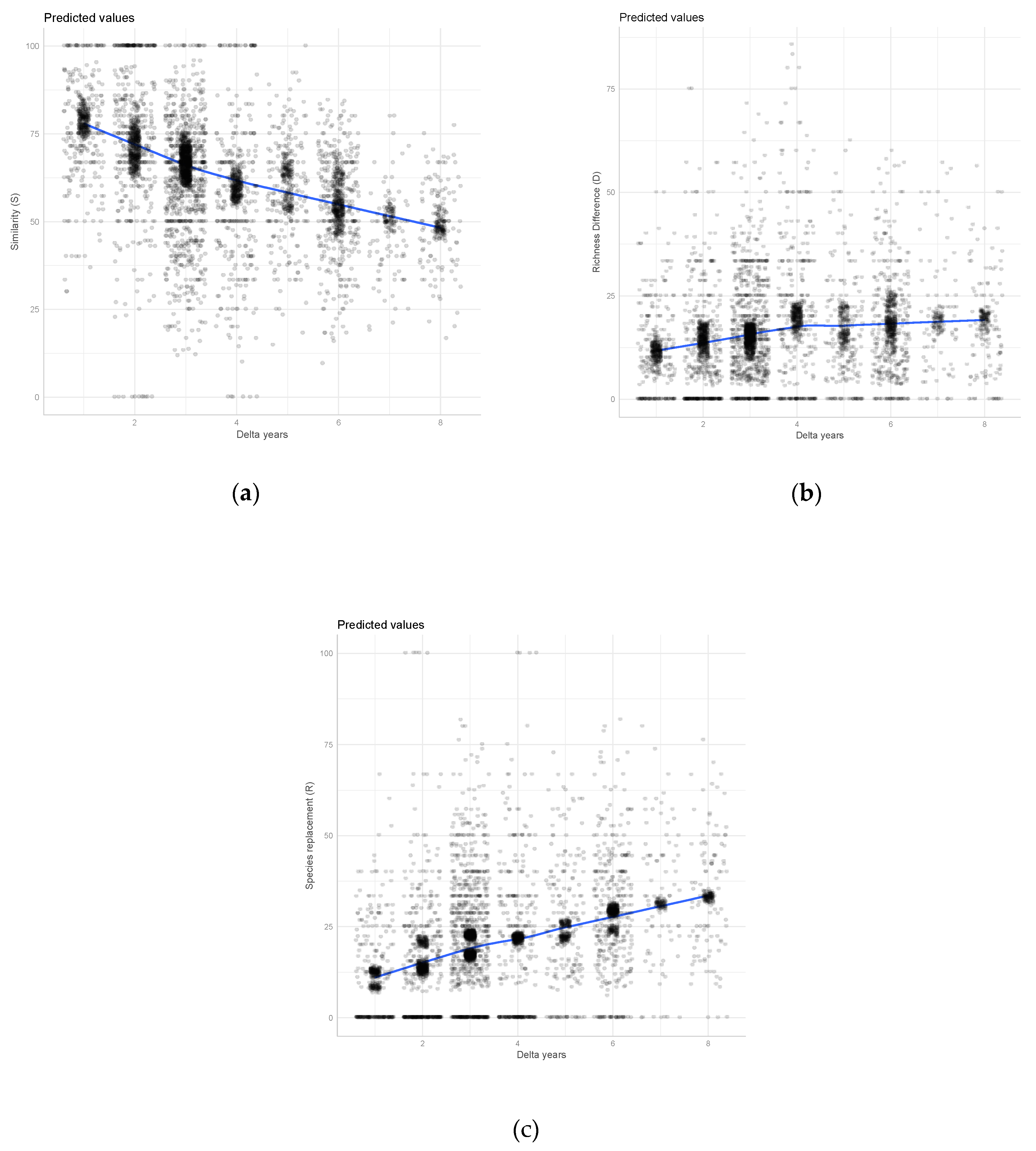
DeltaYears	−0.029	0.003	−9.710 **	0.008	0.002	3.261 **	0.021	0.003	7.169 **
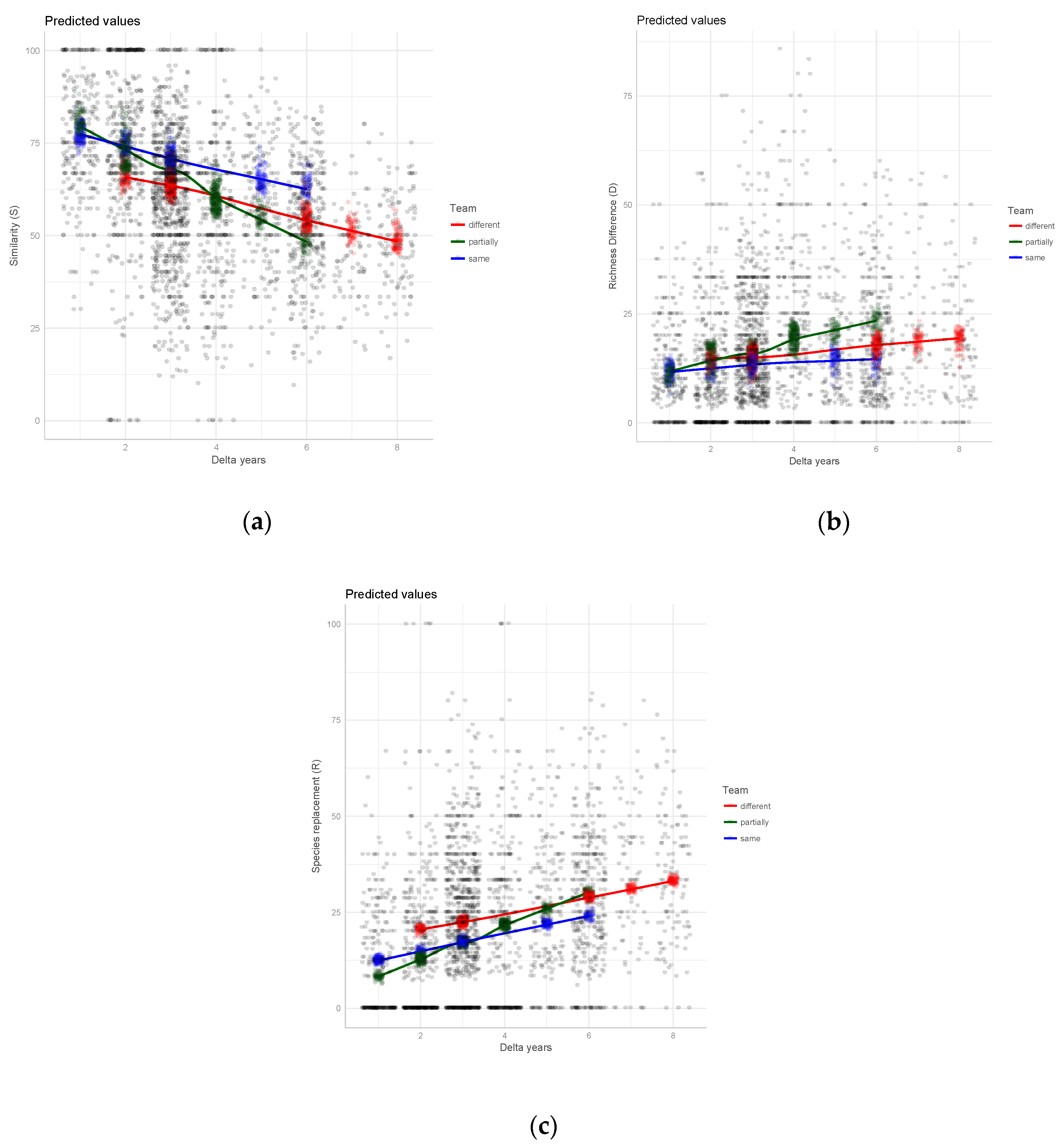
Team ‘partially’ (versus ‘different’)	0.159	0.025	6.480 **	−0.048	0.018	−2.692 **	−0.126	0.023	−5.524 **
Team ‘same’ (versus ‘different’)	0.091	0.027	3.347 **	−0.025	0.019	−1.294 *	−0.063	0.025	−2.554 *
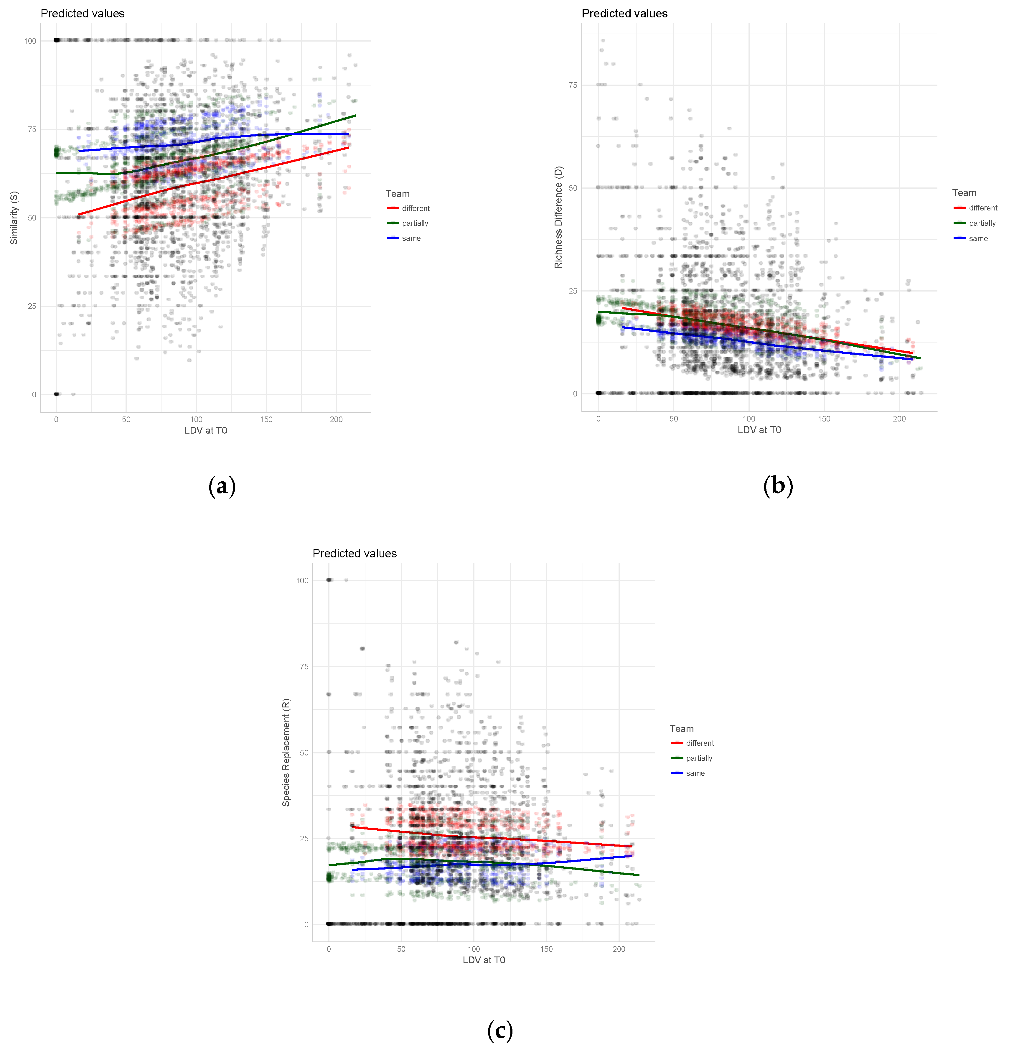
LDV at T0	0.001	0.000	6.772 **	−0.001	0.000	−6.260 **	0.000	0.000	−1.078
DeltaYears:Team ‘partially’ (versus different)	−0.036	0.005	−6.999 **	0.017	0.004	4.204 **	0.023	0.005	4.561 **
DeltaYears:Team ‘same’ (versus ‘different’)	−0.003	0.006	−0.505	0.000	0.005	0.051	0.003	0.006	0.488

). Delta years and team composition consistently showed significant effects on S, D, and R. Particularly, both the “same” and “partially” teams showed significant differences of the three gamma diversity components compared with the “different” teams. The effect of LDV at T₀ was significant for D and S, but not for R. The interaction between delta years and team composition showed significant differences when comparing the “different” versus “partially” teams (Table 2).

When considering the whole dataset independently from the team composition, the SDR analysis revealed that the structure of lichen communities was characterized by a reduction of the values of similarity (S) from 75% to 50% in 8 years, with a more marked reduction in the first 4 years (Figure 1a). The differences in richness (D) among years showed a more regular trend, with values lower than 25% (Figure 1b). An increasing gradient in species replacement (R) from 10% to 35% in the time-span considered was evident (Figure 1c).

We explored the effect of the team composition on the three components of diversity (Figure 2). The decrease in Similarity (S) over time was more marked for the “partially” teams (Figure 2a), ranging from 75% to values lower than 50%, while a more constant trend was evident for the “different” and “same” teams in the repeated surveys, with values ranging respectively from 70% to 50% and from 75% to 65%. Richness Differences (D; Figure 2b) and Species Replacement (R; Figure 2c) in lichen communities showed similar increasing patterns, with a more variable trend for the “partially” teams. R values ranged from 10% to 30%, while D values were always lower than 25%

When considering the SDR values in relation to LDV at T₀ (Figure 3), the three team categories showed increasing values of Similarity (S) ranging from lower to higher values of LDV (from 50% to 75% for the “different” teams; 60% to 80% for the “partially” teams; and from 65 to 75% for the “same” teams). The three team categories showed more marked differences for lower LDV rather than higher ones.

Table 3. List of the common species in the dataset, with their relative values of agreement among the different surveys and the pairwise comparison between the three team categories. The names of the species with significant differences among teams are reported in bold. Nomenclature according to Nimis [43].

Species	Average Percentage Agreement
	Total	Team “different”	Team “partially”	Team “same”
Ramalina fraxinea (L.) Ach.	39	19 a	48 b	51 b
Amandinea punctata (Hoffm.) Coppins & Scheid	40	22 a	48 b	49 b
Candelariella xanthostigma (Ach.) Lettau	42	41 a	43 a	44 a
Caloplaca ferruginea (Huds.) Th. Fr.	45	50 a	44 a	39 a
Evernia prunastri (L.) Ach.	45	52 a	40 a	46 a
Physcia biziana (A. Massal.) Zahlbr. var. biziana	46	20 a	73 b	39 a
Candelariella reflexa (Nyl.) Lettau	46	44 a	50 a	43 a
Ramalina fastigiata (Pers.) Ach.	47	50 a	51 a	34 a
Phlyctis argena (Spreng.) Flot.	47	63 b	34 a	51 ab
Pertusaria pustulata (Ach.) Duby	54	32 a	59 b	61 b
Lecanora expallens Ach.	54	41 a	65 b	53 ab
Normandina pulchella	56	46 a	68 a	47 a
Lepra amara (Ach.) Hafenller	59	60 a	58 a	57 a
Flavoparmelia soredians (Nyl.) Hale	60	46 a	67 a	66 a
Candelaria concolor (Dicks.) Stein	61	56 a	63 a	61 a
Physconia grisea (Lam.) Poelt	64	54 a	75 b	58 a
Melanelixia subaurifera (Nyl) O. Blanco, A. Crespo, Divakar, Essl., D. Hawksw. & Lumbsch	66	60 a	71 a	67 a
Physcia aipolia (Humb.) Fürnr	67	55 a	73 b	71 b
Punctelia subrudecta (Nyl.) Krog	68	68 a	68 a	67 a
Parmelina tiliacea Taylor	70	73 a	67 a	70 a
Lecanora chlarotera Nyl.	71	69 a	68 a	77 a
Parmotrema perlatum (Huds.) M. Choisy	73	69 a	76 a	71 a
Parmelia sulcata (Taylor)	74	77 a	70 a	75 a
Pertusaria albescens (Huds.) M. Choisy & Werner	75	68 a	100 b	82 ab
Lecidella elaeochroma (Ach.) M. Choisy	75	73 a	74 a	81 a
Physconia distorta (With.) J.R. Laundon	76	75 a	75 a	77 a
Xanthoria parietina (L.) Th. Fr.	78	73 a	82 a	76 a
Hyperphyscia adglutinata (Flörke) H. Mayrhofer & Poelt	78	64 a	88 b	79 b
Flavoparmelia caperata (L.) Hale	82	85 a	79 a	84 a
Physcia adscendens H. Oliver	87	83 a	89 a	87 a

^ab Same letters correspond to homogeneous groups (p > 0.05) according to an LSD Fischer post-hoc test.

reports a list of the 30 most common species in the dataset, with their relative values of agreement among the different surveys and the pairwise comparison between the three categories of teams. Average agreement ranged from 39% to 87%, with 9 species showing values lower than 50%. Ten species showed significant differences among teams. Five of these showed the lowest values in the trees sampled by the “different” teams (p < 0.05) with respect to the other two team categories.

Similar results were also evident for the group of rare species (

Table 4. List of the rare species in the dataset, with their relative values of agreement among the different surveys and the pairwise comparison between the three team categories. The names of the species with significant differences among teams are reported in bold. Nomenclature according to Nimis [43].

Species	Average Agreement
	Total	Team “different”	Team “partially”	Team “same”
Caloplaca pyracea (Ach.) Zwackh.	10	10 a	11 a	8 a
Physcia tenella (Scop.) DC.	14	0 a	21 a	8 a
Buellia griseovirens (Sm.) Almb.	15	5 a	24 a	20 a
Leprocaulon microscopicum (Vill.) Gams	16	20 a	19 a	0 a
Physcia leptalea (Ach.) DC.	17	23 a	11 a	22 a
Naetrocymbe punctiformis (Pers.) R.C. Harris	20	14 a	25 a	16 a
Physconia perisidiosa (Erichsen) Moberg	24	25 a	20 a	32 a
Lecanora argentata (Ach.) Malme	27	5 a	32 b	39 b
Gyalecta truncigena (Ach.) Hepp	27	38 b	11 a	44 ab
Tephromela atra (Huds.) Hafellner	27	13 a	33 b	37 b
Melanelixia fuliginosa (Duby) O. Blanco, A. Crespo, Divakar, Essl., D. Hawksw. and Lumbsch	30	38 a	28 a	25 a
Lecanora hagenii (Ach.) Ach.	30	20 a	41 a	28 a
Ramalina farinacea (L.) Ach.	31	47 b	17 a	29 ab
Pertusaria hymenea (Ach.) Schaer	31	40 a	17 a	47 a
Bacidia rubella (Hoffm.) A. Massal	35	37a	40 a	21 a
Physconia servitii (Nádv.) Poelt	35	18 a	47 b	39 ab
Phaeophyscia orbicularis (Neck.) Moberg	36	17 a	46 b	47 b
Lecanora horiza (Ach.) Linds.	39	28 a	44 a	43 a
Phaeophyscia hirsuta (Mereschk.) Moberg	40	45 b	27 a	58 b
Collema furfuraceum Du Rietz	48	40 a	49 a	58 a
Pertusaria pertusa (L.) Tuck.	48	46 a	47 a	53 a
Caloplaca cerinelloides (Erichsen) Poelt	49	29 a	62 a	50 a
Physcia clementei (Turner) Lynge	49	27 a	53 a	58 a
Pertusaria flavida (DC.) J.R. Laundon	50	27 a	56 b	71 b
Lecanora carpinea (L.) Vain.	50	48 a	56 a	45 a
Dendrographa decolorans (Sm.) Ertz and Tehler	52	35 a	58 b	48 ab
Pleurosticta acetabulum (Neck.) Elix & Lumbsch	53	45 a	67 a	39 a
Diploicia canescens (Dicks.) A. Massal.	55	38 a	60 a	74 a
Lecanora symmicta (Ach.) Ach.	55	39 a	67 b	58 ab
Heterodermia obscurata (Nyl.) Trevis.	60	33 a	76 b	63 b
Chrysothrix candelaris (L.) J.R. Laundon	61	35 a	80 b	67 b
Parmotrema reticulatum (Taylor) M. Choisy	64	66 a	61 a	68 a
Opegrapha niveoatra (Borrer) J.R. Laundon	98	100 a	97 a	100 a

^ab Same letters correspond to homogeneous groups (p > 0.05) according to a LSD Fischer post-hoc test.

; 33 species), with average agreement ranging from 10% to 98%. Twenty-three of them showed values lower than 50%. Twelve species showed significant differences among teams. Six of these had significantly lower values (p < 0.05) in the “different” teams. Among them, were four crustose lichens (Lecanora argentata, Tephromela atra, Pertusaria flavida, and Chrysothrix candelaris), and two narrow-lobed foliose lichens (Phaeophyscia orbicularis and Heterodermia obscurata).

4. Discussion

Lichen biomonitoring is a standardized method that requires high levels of taxonomic knowledge. Therefore, lichenologists in charge of data collection can influence the quality of the results [32].

At a small scale of observation, as that used for single plots in lichen biomonitoring, observer error is expected to be high and might overcome the variance related to the target environmental signal (e.g., pollution) [44].

Although several tests [30,31,32] evaluated the accuracy of single operators, none have assessed the results obtained in cases of rotation or partial change of team composition in long-term biomonitoring programs. To fill this gap of knowledge, in this work we investigated temporal variations of epiphytic lichen diversity in relation to the composition of the teams involved in repeated biomonitoring surveys.

In general, our study highlighted significant effects on diversity assessments due to team composition. These effects will have to be taken into due consideration because they could potentially lead to errors in the interpretation of the data obtained. However, detailed analysis of these effects will allow targeted activities to be planned to mitigate this risk. Furthermore, the observed effects are diversified according to whether quantitative (e.g., diversity) or qualitative (e.g., species composition and species ecology) aspects are taken into account.

4.1. Quantitative Aspects of Lichen Diversity

Probabilistic sampling based on the location of plots and sub-plots within a survey area can provide reliable estimates of the overall diversity, even though a given number of rare species are often unrecorded [44]. Among several descriptors of lichen diversity, Giordani et al. [25] showed that the components of gamma diversity are important to highlight temporal and spatial variation in epiphytic lichen communities and to follow their progress over time. In the present work, we compared pairs of subsequent surveys carried out at time intervals ranging from 1 to 8 years. In these situations, our results showed an increase over time in the Species Replacement (R), corresponding to a decrease in Similarity (S) and a constant trend of the Richness Difference (D). Taking into consideration the composition of the teams in more detail, it has emerged that R and D increased over time both for the “different” and “same” teams with a comparable trend. In contrast, for the “partially” teams the trend was significantly different compared with the other team categories, determining a less controllable non-sampling error. Correspondingly, the decrease of S after 6 years was more marked for the “different” and “partially” teams (about 50%), while, at the same time, the samplings undertaken by the “same” teams were more similar to each other.

It should be carefully taken into account that SDR values describe variations in lichen communities ascribable to at least four major factors, including natural succession of communities [27], variations due to the increase/decrease of pollution [2,45], and sampling and non-sampling errors (operator effect) [26,33]. As the evaluation of the effects of environmental changes is based on these variations, it is fundamental to understand the contribution of each factor. Several studies have addressed the first three aspects, whereas less is known about the last one. Our results do not allow us to discern the effect of population dynamics or pollution, but we can still observe significant variations according to the time elapsed between two surveys and depending on the team composition.

In contrast to what we would have expected, the differences between teams were more evident on trees with low Lichen Diversity Values (S = 70% in the “same” teams versus S = 50% in the “different” teams). The differences between teams were reduced in case of high diversity, with values of S approximately equal to 70% for all types of teams. This is probably due to the fact that in conditions of high alteration the lichen thalli are often wrecked and scarcely recognizable even to skilled operators. Errors of identification and/or overlook of these species could lead to important underestimates of diversity. This is in accordance with what observed by Ellis and Coppins [44]. These authors noted that the confirmation of atypical specimens is particularly difficult when using small subsamples (as in the case of lichen biomonitoring). As altered study areas are often the main targets of biomonitoring programs, it is a priority to implement countermeasures to increase the similarity in such conditions (see paragraph 4.3). In contrast, the positive aspect is that, under conditions of high LDV values, greater homogeneity was observed between the results produced by the different categories of teams. Based on our results we cannot provide a direct assessment of the taxonomic accuracy reached in the surveys considered. However, high similarity values guarantee good data comparability and reduce the risk of misinterpretation of results [26].

4.2. Taxonomic Agreement in Relation to Team Composition

From what was discussed in the previous paragraph, we can state that the results of biomonitoring programs are generally comparable when considering quantitative aspects (e.g., gamma diversity components or LDV). However, would we obtain the same information if we took into account species ecological requirements (e.g., nitrophilous and acidophilus species)? As shown in Table 3, some species with low agreement were very common species, but ones that can be frequently confused with similar species that differ in their ecology (e.g., Flavoparmelia caperata versus Flavoparmelia soredians, Amandinea punctata versus Lecidella elaeochroma, or Parmotrema perlatum versus Parmotrema reticulatum). In general, species with low agreement in the “different” team category are difficult to identify in the field when present on tree trunks with poorly developed thalli. Most of them are crustose lichens (e.g., Pertusaria pustulata, Lecanora argentata), or foliose narrow-lobed ones (e.g., Physcia aipolia, Phaeophyscia orbicularis). This fact can lead to erroneous considerations about community composition (e.g., acidophitic versus nitrophytic) and about the factors that might have determined it [46,47,48,49,50,51]. This issue is crucial to prevent the loss of information related to the ecology of the species. In modern biomonitoring, the analysis of ecological requirements of the lichen communities is pivotal for a comprehensive interpretation of the drivers that might have caused observed variations [52,53]. It has been demonstrated that species and/or functional traits react differently to anthropogenic disturbances [14,16,54,55,56]. Several studies focused on lichen biota shifts due to decreasing SO₂ concentrations and increasing nitrogen pollution confirmed the relevance of such information [50,57,58,59,60].

Even though there may be disagreement in the identification of very common species, in our study, we generally observed that the overall agreement was higher for common species compared with rare ones (Table 3 and Table 4). In some cases, it has been observed that common species can be overlooked, because the attention of the operators is often focused on infrequent species [44]. In ecological sampling based on sub-samples, rare species are unrecorded due to their low probability of being included within the sample units. In our study, for both common and rare species, we observed significant differences between team categories. In fact, most of the common species in the dataset (70%) showed levels of agreement > 50%, while the opposite is true for the rare ones, with only 30% of the species exceeding this level of agreement. This is probably related to the fact that common species can be easily identified in the field based on the acquired experience of the operators. In contrast, rare species are more sporadic, and often small; many of them are critical taxa, often difficult to identify, less familiar for operators, especially if they do not have sufficient knowledge of the local lichen biota [32,33]. Accordingly, it has been demonstrated that the familiarity with local diversity is a critical factor that can influence the number of species detected by different operators [33,44,61].

4.3. Recommandations

Our results show that the surveys conducted by the “same” teams have the highest agreements. However, as biomonitoring programs are open to public tenders and last several years, it is not always possible that all the surveys are carried out by the same team composition. These results highlight the importance of the continuous training of the personnel involved. Particularly, attention must be paid to the following aspects:

• Periodic ring test organization. The effectiveness of this activity is achieved only if the intercalibration exercise is regularly repeated over time [34]. In fact, it has been shown that a decrease, even if limited, of taxonomic accuracy can be observed even in taxonomist experts. The effect of the loss of accuracy is obviously much more evident in trained personnel who have not yet reached a high level of experience.
• Calibrations of the operators within the same program. This calibration activity should be done between the two operators composing the team carrying out the same survey and/or among teams involved in different surveys of the same program. Additionally, external skilled personnel could also be involved as a control team to provide a further level of quality assurance. This activity would minimize the differences attributable to non-sampling errors within the same area of study (e.g., between high and low diversity areas) and/or subsequent surveys of the same monitoring program. The main problems in applying these interventions can be identified in the difficulty of planning long-term activities and involving people who have worked at different times.
• Preparatory training aimed at improving the knowledge of local lichen biota. In many cases, the operators involved in the sampling of a study area may not have specific knowledge of the local biota. This is particularly true in case of operators with low level of experience, but even skilled lichenologists may not be able to maintain a high level of taxonomic accuracy without preparatory and intensive training on the local lichen biota.
• Staff training on critical taxonomic groups. On the basis of the results reported in this study, it is evident that specialized training on some critical groups of species (e.g., genera of crustose lichens) can lead to a substantial improvement of the agreement between operators. Although recommendable, the organization of advanced workshops involves a considerable logistical effort in the retrieval of materials, laboratory equipment and the availability of experts able to clarify doubts on critical species. As a further option, experts could be invited to participate in the surveys of the monitoring program, even though this may lead to an increase of the total cost of the program.

References

- Nash, T.H. Lichen Biology; Cambridge University Press: Leiden, The Netherlands, 2006; ISBN 978-0-511-41407-7. [Google Scholar]
- Nimis, P.L.; Scheidegger, C.; Wolseley, P.A. (Eds.) Monitoring with Lichens—Monitoring Lichens; Springer: Dordrecht, The Netherlands, 2002; pp. 1–4. ISBN 978-1-4020-0430-8. [Google Scholar]
- CEN. Ambient Air—Biomonitoring with Lichens—Assessing Epiphytic Lichen Diversity; CEN: Brussels, Belgium, 2014. [Google Scholar]
- ANPA. I.B.L. Indice di Biodiversità Lichenica; Manuali e linee guida; ANPA: Roma, Italy, 2001; ISBN 88-448-0256-2. [Google Scholar]
- Asta, J.; Erhardt, W.; Ferretti, M.; Fornasier, F.; Kirschbaum, U.; Nimis, P.L.; Purvis, O.W.; Pirintsos, S.; Scheidegger, C.; Van Haluwyn, C.; et al. Mapping Lichen Diversity as an Indicator of Environmental Quality. In Monitoring with Lichens—Monitoring Lichens; Nimis, P.L., Scheidegger, C., Wolseley, P.A., Eds.; NATO Science Series; Springer: Dordrecht, The Netherlands, 2002; pp. 273–279. ISBN 978-94-010-0423-7. [Google Scholar]
- Giordani, P.; Brunialti, G. Sampling and Interpreting Lichen Diversity Data for Biomonitoring Purposes. In Recent Advances in Lichenology; Upreti, D.K., Divakar, P.K., Shukla, V., Bajpai, R., Eds.; Springer: New Delhi, India, 2015; pp. 19–46. ISBN 978-81-322-2180-7. [Google Scholar]
- Kricke, R.; Loppi, S. Bioindication: The I.A.P. Approach. In Monitoring with Lichens—Monitoring Lichens; Nimis, P.L., Scheidegger, C., Wolseley, P.A., Eds.; Springer: Dordrecht, The Netherlands, 2002; pp. 21–37. ISBN 978-1-4020-0430-8. [Google Scholar]
- Nimis, P.L.; Purvis, O.W. Monitoring Lichens as Indicators of Pollution. In Monitoring with Lichens—Monitoring Lichens; Nimis, P.L., Scheidegger, C., Wolseley, P.A., Eds.; Springer: Dordrecht, The Netherlands, 2002; pp. 7–10. ISBN 978-1-4020-0430-8. [Google Scholar]
- Will-Wolf, S.; Geiser, L.H.; Neitlich, P.; Reis, A.H. Forest lichen communities and environment—How consistent are relationships across scales? J. Veg. Sci. 2009, 17, 171–184. [Google Scholar]
- Will-Wolf, S.; Esseen, P.-A.; Neitlich, P. Monitoring Biodiversity and Ecosystem Function: Forests. In Monitoring with Lichens—Monitoring Lichens; Nimis, P.L., Scheidegger, C., Wolseley, P.A., Eds.; Springer: Dordrecht, The Netherlands, 2002; pp. 203–222. ISBN 978-1-4020-0430-8. [Google Scholar]
- Nascimbene, J.; Thor, G.; Nimis, P.L. Effects of forest management on epiphytic lichens in temperate deciduous forests of Europe—A review. For. Ecol. Manag. 2013, 298, 27–38. [Google Scholar] [CrossRef]
- Maes, W.H.; Fontaine, M.; Rongé, K.; Hermy, M.; Muys, B. A quantitative indicator framework for stand level evaluation and monitoring of environmentally sustainable forest management. Ecol. Indic. 2011, 11, 468–479. [Google Scholar] [CrossRef]
- Giordani, P. Assessing the effects of forest management on epiphytic lichens in coppiced forests using different indicators. Plant Biosyst. Int. J. Deal. Asp. Plant Biol. 2012, 146, 628–637. [Google Scholar] [CrossRef]
- Pinho, P.; Bergamini, A.; Carvalho, P.; Branquinho, C.; Stofer, S.; Scheidegger, C.; Máguas, C. Lichen functional groups as ecological indicators of the effects of land-use in Mediterranean ecosystems. Ecol. Indic. 2012, 15, 36–42. [Google Scholar] [CrossRef]
- Wolseley, P.A.; Stofer, S.; Mitchell, R.; Truscott, A.-M.; Vanbergen, A.; Chimonides, J.; Scheidegger, C. Variation of lichen communities with landuse in Aberdeenshire, UK. Lichenologist 2006, 38, 307. [Google Scholar] [CrossRef]
- Stofer, S.; Bergamini, A.; Aragón, G.; Carvalho, P.; Coppins, B.J.; Davey, S.; Dietrich, M.; Farkas, E.; Kärkkäinen, K.; Keller, C.; et al. Species richness of lichen functional groups in relation to land use intensity. Lichenologist 2006, 38, 331. [Google Scholar] [CrossRef]
- Ellis, C.J.; Eaton, S.; Theodoropoulos, M.; Coppins, B.J.; Seaward, M.R.D.; Simkin, J. Response of epiphytic lichens to 21st Century climate change and tree disease scenarios. Biol. Conserv. 2014, 180, 153–164. [Google Scholar] [CrossRef]
- Geiser, L.H.; Neitlich, P.N. Air pollution and climate gradients in western Oregon and Washington indicated by epiphytic macrolichens. Environ. Pollut. 2007, 145, 203–218. [Google Scholar] [CrossRef]
- Giordani, P.; Incerti, G. The influence of climate on the distribution of lichens: A case study in a borderline area (Liguria, NW Italy). Plant Ecol. 2008, 195, 257–272. [Google Scholar] [CrossRef]
- Matos, P.; Geiser, L.; Hardman, A.; Glavich, D.; Pinho, P.; Nunes, A.; Soares, A.M.V.M.; Branquinho, C. Tracking global change using lichen diversity: Towards a global-scale ecological indicator. Methods Ecol. Evol. 2017, 8, 788–798. [Google Scholar] [CrossRef]
- Matos, P.; Pinho, P.; Aragón, G.; Martínez, I.; Nunes, A.; Soares, A.M.V.M.; Branquinho, C. Lichen traits responding to aridity. J. Ecol. 2015, 103, 451–458. [Google Scholar] [CrossRef]
- Ferretti, M.; Brambilla, E.; Brunialti, G.; Fornasier, F.; Mazzali, C.; Giordani, P.; Nimis, P. Reliability of different sampling densities for estimating and mapping lichen diversity in biomonitoring studies. Environ. Pollut. 2004, 127, 249–256. [Google Scholar] [CrossRef]
- Frati, L.; Brunialti, G. Long-Term Biomonitoring with Lichens: Comparing Data from Different Sampling Procedures. Environ. Monit. Assess. 2006, 119, 391–404. [Google Scholar] [CrossRef]
- Giordani, P.; Matteucci, E.; Redana, M.; Ferrarese, A.; Isocrono, D. Unsustainable cattle load in alpine pastures alters the diversity and the composition of lichen functional groups for nitrogen requirement. Fungal Ecol. 2014, 9, 69–72. [Google Scholar] [CrossRef]
- Giordani, P.; Brunialti, G.; Calderisi, M.; Malaspina, P.; Frati, L. Beta diversity and similarity of lichen communities as a sign of the times. Lichenologist 2018, 50, 371–383. [Google Scholar] [CrossRef]
- Ferretti, M.; Erhardt, W. Key Issues in Designing Biomonitoring Programmes. In Monitoring with Lichens—Monitoring Lichens; Nimis, P.L., Scheidegger, C., Wolseley, P.A., Eds.; Springer: Dordrecht, The Netherlands, 2002; pp. 111–139. ISBN 978-1-4020-0430-8. [Google Scholar]
- Barkman, J.J. Phytosociology and Ecology of Cryptogamic Epiphytes: Including a Taxonomic Survey and Description of Their Vegetation Units in Europe; Van Gorcum: Assen, The Netherlands, 1958. [Google Scholar]
- Ribeiro, M.C.; Pinho, P.; Branquinho, C.; Llop, E.; Pereira, M.J. Geostatistical uncertainty of assessing air quality using high-spatial-resolution lichen data: A health study in the urban area of Sines, Portugal. Sci. Total Environ. 2016, 562, 740–750. [Google Scholar] [CrossRef]
- Brunialti, G.; Giordani, P.; Isocrono, D.; Loppi, S. Evaluation of data quality in lichen biomonitoring studies: The Italian experience. Environ. Monit. Assess. 2002, 75, 271–280. [Google Scholar] [CrossRef]
- Brunialti, G.; Frati, L.; Cristofolini, F.; Chiarucci, A.; Giordani, P.; Loppi, S.; Benesperi, R.; Cristofori, A.; Critelli, P.; Di Capua, E.; et al. Can we compare lichen diversity data? A test with skilled teams. Ecol. Indic. 2012, 23, 509–516. [Google Scholar] [CrossRef]
- Cristofolini, F.; Brunialti, G.; Giordani, P.; Nascimbene, J.; Cristofori, A.; Gottardini, E.; Frati, L.; Matos, P.; Batič, F.; Caporale, S.; et al. Towards the adoption of an international standard for biomonitoring with lichens—Consistency of assessment performed by experts from six European countries. Ecol. Indic. 2014, 45, 63–67. [Google Scholar] [CrossRef]
- Giordani, P.; Brunialti, G.; Benesperi, R.; Rizzi, G.; Frati, L.; Modenesi, P. Rapid biodiversity assessment in lichen diversity surveys: Implications for quality assurance. J. Environ. Monit. 2009, 11, 730. [Google Scholar] [CrossRef]
- Mccune, B.; Dey, J.P.; Peck, J.E.; Cassell, D.; Heiman, K.; Will-Wolf, S.; Neitlich, P.N. Repeatability of community data: Species richness versus gradient scores in large-scale lichen studies. Bryologist 1997, 100, 40–46. [Google Scholar] [CrossRef]
- Ferretti, M. Quality assurance: A vital need in ecological monitoring. CAB Rev. Perspect. Agric. Vet. Sci. Nutr. Nat. Resour. 2011, 6. [Google Scholar] [CrossRef]
- Stribling, J.B.; Moulton, S.R.; Lester, G.T. Determining the quality of taxonomic data. J. N. Am. Benthol. Soc. 2003, 22, 621–631. [Google Scholar] [CrossRef]
- Stribling, J.B.; Pavlik, K.L.; Holdsworth, S.M.; Leppo, E.W. Data quality, performance, and uncertainty in taxonomic identification for biological assessments. J. N. Am. Benthol. Soc. 2008, 27, 906–919. [Google Scholar] [CrossRef]
- Contardo, T.; Giordani, P.; Paoli, L.; Vannini, A.; Loppi, S. May lichen biomonitoring of air pollution be used for environmental justice assessment? A case study from an area of N Italy with a municipal solid waste incinerator. Environ. Forensics 2018, 0, 1–12. [Google Scholar] [CrossRef]
- Loppi, S. May the Diversity of Epiphytic Lichens Be Used in Environmental Forensics? Diversity 2019, 11, 36. [Google Scholar] [CrossRef]
- Podani, J.; Schmera, D. A new conceptual and methodological framework for exploring and explaining pattern in presence—Absence data. Oikos 2011, 120, 1625–1638. [Google Scholar] [CrossRef]
- Akaike, H. A Bayesian extension of the minimum AIC procedure of autoregressive model fitting. Biometrika 1979, 66, 237–242. [Google Scholar] [CrossRef]
- Bates, D.; Maechler, M.; Bolker, B.; Walker, S.; Christensen, R.H.B.; Singmann, H.; Dai, B. Package ‘lme4’; R Foundation for Statistical Computing: Vienna, Austria, 2014. [Google Scholar]
- R Core team. R: A Language and Environment for Statistical Computing; R Foundation for Statistical Computing: Vienna, Austria, 2018. [Google Scholar]
- Nimis, P.L. The Lichens of Italy. A Second Annotated Catalogue; EUT: Trieste, Italy, 2016; ISBN 978-88-8303-754-2. [Google Scholar]
- Ellis, C.J.; Coppins, B.J. Taxonomic survey compared to ecological sampling: Are the results consistent for woodland epiphytes? Lichenologist 2017, 49, 141–155. [Google Scholar] [CrossRef]
- Shukla, V.; Upreti, D.K.; Bajpai, R. Lichens to Biomonitor the Environment; Springer: New Delhi, India, 2014. [Google Scholar]
- van Herk, C.M. Bark pH and susceptibility to toxic air pollutants as independent causes of changes in epiphytic lichen composition in space and time. Lichenologist 2001, 33, 419–441. [Google Scholar] [CrossRef]
- Frati, L.; Santoni, S.; Nicolardi, V.; Gaggi, C.; Brunialti, G.; Guttova, A.; Gaudino, S.; Pati, A.; Pirintsos, S.A.; Loppi, S. Lichen biomonitoring of ammonia emission and nitrogen deposition around a pig stockfarm. Environ. Pollut. 2007, 146, 311–316. [Google Scholar] [CrossRef]
- Pinho, P.; Theobald, M.R.; Dias, T.; Tang, Y.S.; Cruz, C.; Martins-Loução, M.A.; Máguas, C.; Sutton, M.; Branquinho, C. Critical loads of nitrogen deposition and critical levels of atmospheric ammonia for semi-natural Mediterranean evergreen woodlands. Biogeosciences 2012, 9, 1205–1215. [Google Scholar] [CrossRef]
- Pinho, P.; Dias, T.; Cruz, C.; Sim Tang, Y.; Sutton, M.A.; Martins-Loução, M.-A.; Máguas, C.; Branquinho, C. Using lichen functional diversity to assess the effects of atmospheric ammonia in Mediterranean woodlands. J. Appl. Ecol. 2011, 48, 1107–1116. [Google Scholar] [CrossRef]
- Davies, L.; Bates, J.W.; Bell, J.N.B.; James, P.W.; Purvis, O.W. Diversity and sensitivity of epiphytes to oxides of nitrogen in London. Environ. Pollut. 2007, 146, 299–310. [Google Scholar] [CrossRef]
- Munzi, S.; Cruz, C.; Branquinho, C.; Pinho, P.; Leith, I.D.; Sheppard, L.J. Can ammonia tolerance amongst lichen functional groups be explained by physiological responses? Environ. Pollut. 2014, 187, 206–209. [Google Scholar] [CrossRef]
- Llop, E.; Pinho, P.; Matos, P.; Pereira, M.J.; Branquinho, C. The use of lichen functional groups as indicators of air quality in a Mediterranean urban environment. Ecol. Indic. 2012, 13, 215–221. [Google Scholar] [CrossRef]
- Pinho, P.; Llop, E.; Ribeiro, M.C.; Cruz, C.; Soares, A.; Pereira, M.J.; Branquinho, C. Tools for determining critical levels of atmospheric ammonia under the influence of multiple disturbances. Environ. Pollut. 2014, 188, 88–93. [Google Scholar] [CrossRef]
- Munzi, S.; Correia, O.; Silva, P.; Lopes, N.; Freitas, C.; Branquinho, C.; Pinho, P. Lichens as ecological indicators in urban areas: Beyond the effects of pollutants. J. Appl. Ecol. 2014, 51, 1750–1757. [Google Scholar] [CrossRef]
- Giordani, P.; Brunialti, G.; Bacaro, G.; Nascimbene, J. Functional traits of epiphytic lichens as potential indicators of environmental conditions in forest ecosystems. Ecol. Indic. 2012, 18, 413–420. [Google Scholar] [CrossRef]
- Ellis, C.J.; Coppins, B.J. Contrasting functional traits maintain lichen epiphyte diversity in response to climate and autogenic succession. J. Biogeogr. 2006, 33, 1643–1656. [Google Scholar] [CrossRef]
- Van Herk, C.M.; Mathijssen-Spiekman, E.A.M.; De Zwart, D. Long distance nitrogen air pollution effects on lichens in Europe. Lichenologist 2003, 35, 347–359. [Google Scholar] [CrossRef]
- Cristofolini, F.; Giordani, P.; Gottardini, E.; Modenesi, P. The response of epiphytic lichens to air pollution and subsets of ecological predictors: A case study from the Italian Prealps. Environ. Pollut. 2008, 151, 308–317. [Google Scholar] [CrossRef]
- Hauck, M. Susceptibility to acidic precipitation contributes to the decline of the terricolous lichens Cetraria aculeata and Cetraria islandica in central Europe. Environ. Pollut. 2008, 152, 731–735. [Google Scholar] [CrossRef]
- Giordani, P.; Malaspina, P. Do tree-related factors mediate the response of lichen functional groups to eutrophication? Plant Biosyst. Int. J. Deal. Asp. Plant Biol. 2017, 151, 1062–1072. [Google Scholar] [CrossRef]
- Archaux, F.; Camaret, S.; Dupouey, J.-L.; Ulrich, E.; Corcket, E.; Bourjot, L.; Brêthes, A.; Chevalier, R.; Dobremez, J.-F.; Dumas, Y.; et al. Can We Reliably Estimate Species Richness with Large Plots? An Assessment through Calibration Training. Plant Ecol. 2009, 203, 303–315. [Google Scholar] [CrossRef]