Introduction
The Bayer Process is presently the most economic means for alumina production and promises to be so for many years to come. The process can be most simply described by the following steps:
dissolution of extractable aluminium bearing minerals from bauxite in sodium hydroxide at elevated temperatures (and pressures);
removal of insoluble impurities and clarification of the remaining solution;
precipitation of pure gibbsite from the clarified solution by cooling to highly supersaturated levels and seeding with previously precipitated gibbsite crystals;
calcination of the crystallised gibbsite at 1100°C to remove chemically bound water to produce alumina.
As an industry, the Bayer process is quite mature, but there are still many fundamental phenomena occurring in the process that are not very well understood. For example, the speciation and crystallisation mechanisms in Bayer solutions or liquors are still the subjects of considerable conjecture [
1,
2]. A similar case also exists for models describing gibbsite solubility in Bayer liquors which are as varied in their approaches as the are ubiquitous. Because the rate and extent of gibbsite precipitation from the Bayer liquor strongly depends on the level of supersaturation, the control and optimisation of this component of the Bayer process is greatly facilitated by a good understanding of gibbsite solubility. The motivation for developing a corresponding descriptive model is therefore obvious.
Owing to their particular idiosyncrasies, some of the gibbsite solubility models appearing in the literature are limited in their application to one extent or another (See Ref. 3 for a review). One common limitation, however, is that most models do not account for the effects of dissolved impurities which can have significant impact on gibbsite solubility. Organic and inorganic impurities can enter the liquor circuit from several different sources such as the raw bauxite ore for example. The scarcity of available models that adequately incorporate impurity effects is, in itself, testimony to the difficulty of the problem. Possibly the most ambitious attempt to derive a flexible solubility model was presented by Rosenberg and Healy (RH) [
3]. Following on from concepts introduced by Bouzat and Philiponneau [
4] they developed a model based on thermodynamic principles describing the equilibrium equation:
The effect of impurities was then accounted for by considering their effect on activity coefficients. Parameters of the final model equation were calibrated by fitting experimental data and further validated indicating sound predictive properties. One of the problems was, however, that the model tended to fail at high and low caustic concentrations which may have been due to either analytical errors or inappropriate activity coefficients for describing the system at the extremes. A subtler problem was revealed when investigating the application of the RH model to Gove process liquors. In this case, model predictions deviated significantly from the experimentally measured gibbsite equilibrium solubility concentrations. A possible explanation for this considerably large discrepancy may involve the solution phase speciation of impurities. It would not be unreasonable to expect that the Worsley refinery liquors used by RH may have a significantly contrasting impurity composition to Gove liquors due predominantly to the different raw materials entering the respective processes. Gove bauxite, for example, is starkly different in character to the Darling Range bauxite used at Worsley. Other raw materials, such as caustic soda as well as the way in which impurities are treated may also vary considerably from plant to plant. The variability of impurity species that may be present in Bayer Liquors of different origins renders the development of a universally applicable, phenomenological solubility model practically impossible.
In this paper we investigate an alternative method of developing a gibbsite solubility model based on the Group Method of Data Handling (GMDH) algorithm [
5,
6]. The GMDH network is a learning machine based on the principle of heuristic self-organisation. Unlike classical neural network modelling, GMDH elegantly self determines a network structure of active neurons (or transfer functions) automatically while synthesising an analytical model relating the input basis data to the associated output data. During the network construction, relevant input variables of the system are also determined while insignificant variables are discarded in a process of genetic inheritance, mutation and selection. The GMDH
ansatz realises a powerful method for constructing accurate model equations with little or no
a priori knowledge of the system being modelled.
Experiment Details
The experimental method employed in the present investigation followed a similar strategy to Rosenberg and Healy [3]. The main objective of the experimental work was to simulate typical plant conditions rather than perform completely controlled experiments based on fully synthetic liquor systems. Gibbsite solubility measurements were therefore carried out using spent Bayer liquor sampled from the Gove refinery as a basis. Liquor compositions were then manipulated by a number of means such as the addition of soluble chemicals, addition of synthetic liquor, addition of water and the evaporation of liquors. As well as the liquor impurities considered by RH, the effect of fluoride concentration was also taken into account in this work. 124 equilibrium gibbsite solubility tests were carried out exploring the range of liquor conditions outlined in
Table 1. A strong association between the impurity anions and sodium is expected. It is therefore conventional to express impurities in terms of their sodium salts. Industry standard methods were used for analysing the test liquors at their final equilibrium conditions. This included thermal titration for determining Al
2O
3, Na
2CO
3 and caustic concentrations [7] and capillary ion analysis for the anions Cl- and
. Total organic carbon was analysed on a Dohrmann DC-180 Carbon Analyser which utilises the ultra-violet promoted persulfate oxidation method. Fluoride analysis was carried out by burning samples in a modified oxy-hydrogen burner. The fluoride was then scrubbed out of the combustion products and concentrations determined in a conventional manner [
8].
There are no strict industry conventions for expressing concentrations and here C stands for caustic concentration expressed as Na2O, dissolved gibbsite is given in terms of Al2O3 and TOC is the Total Organic Carbon as g/L carbon.
GMDH Modelling of Experimental Data
GMDH is essentially a self-organising network of active neurons or transfer functions. The network architecture is fully self-determined by the algorithm itself. The final network consists of the zeroth layer or input data and the final output layer which are connected through a network structure which is made up of several layers of active neurons of progressively increasing complexity. The basic approach of GMDH is that each neuron in the network receives input from exactly two other neurons with the exception of the neurons representing the input layer. The two inputs,
and
are then combined to produce a partial descriptor based on the simple quadratic transfer function
where the coefficients
a..f are determined statistically and are unique for each transfer function. The coefficients can be thought of as analogous to weights found in other types of neural networks.
The network of transfer functions is constructed one layer at a time. The first network layer consists of functions of each possible pair of n input variables (zeroth layer) resulting in n (n-1)/2 neurons. The second layer is created using inputs from the first layer and so on. The first network layer therefore consists of a set of quadratic functions of the input variables, the second layer involves fourth degree polynomials, the third layer includes eighth degree polynomials etc. A selection process is employed to limit the size of the network by culling neurons at each layer based on a performance criterion. The way in which this is done represents an important feature of the GMDH algorithm. While the parameters of each transfer function are estimated using a training set of observations to optimise the behaviour of the partial descriptor, a separate testing set is used to rank and select the best partial descriptors of each network layer. This approach guarantees objectivity during the model construction process and serves to avoid overfitting. A pre-defined number of surviving neurons are preserved which then mutate to form the subsequent layer as described above. The algorithm automatically terminates once the performance of the network begins to deteriorate.
Unlike other types of neural network approaches to modelling data, GMDH provides a fully portable, symbolic description of the final network or model in the form of a polynomial function of the selected, relevant input variables. Specifically, a Volterra series is generated in the form
where
X(
,
, ….,
) is the vector of input variables and
A(
,
,….,
) is the vector of summand coefficients.
Being an inductive process, GMDH adheres to the principle of Occam’s razor which advocates a parsimonious model in contrast to other neural network approaches which systematically tend to overfit data. This is an important attribute when attempting to identify relevant input variables to a complex system such as the present case of determining which impurities influence gibbsite solubility.
The modelling of the solubility data employed a twice multi-layered network structure GMDH variant as implemented in the KnowledgeMiner program package [
9]. The mechanism of layer-breakthrough was employed to allow all input variables and selected partial descriptors from previous layers to be reintroduced into subsequent network layers regardless of whether or not they were selected in the most recent network layer. This approach is more computationally demanding but provides considerably greater flexibility in the model construction process by avoiding premature elimination of input variables or selected partial models.
To develop the present gibbsite solubility model, temperature, caustic concentration and the concentration of each impurity provided the set of input vectors. The experimentally determined equilibrium gibbsite solubility for each set of input conditions represented the output to be modelled. With these raw data provided in tabular form, the GMDH algorithm was left more or less to its own devices to formulate an appropriate model. The resulting GMDH network is presented in algebraic form in Ref 10.
Results and Discussion
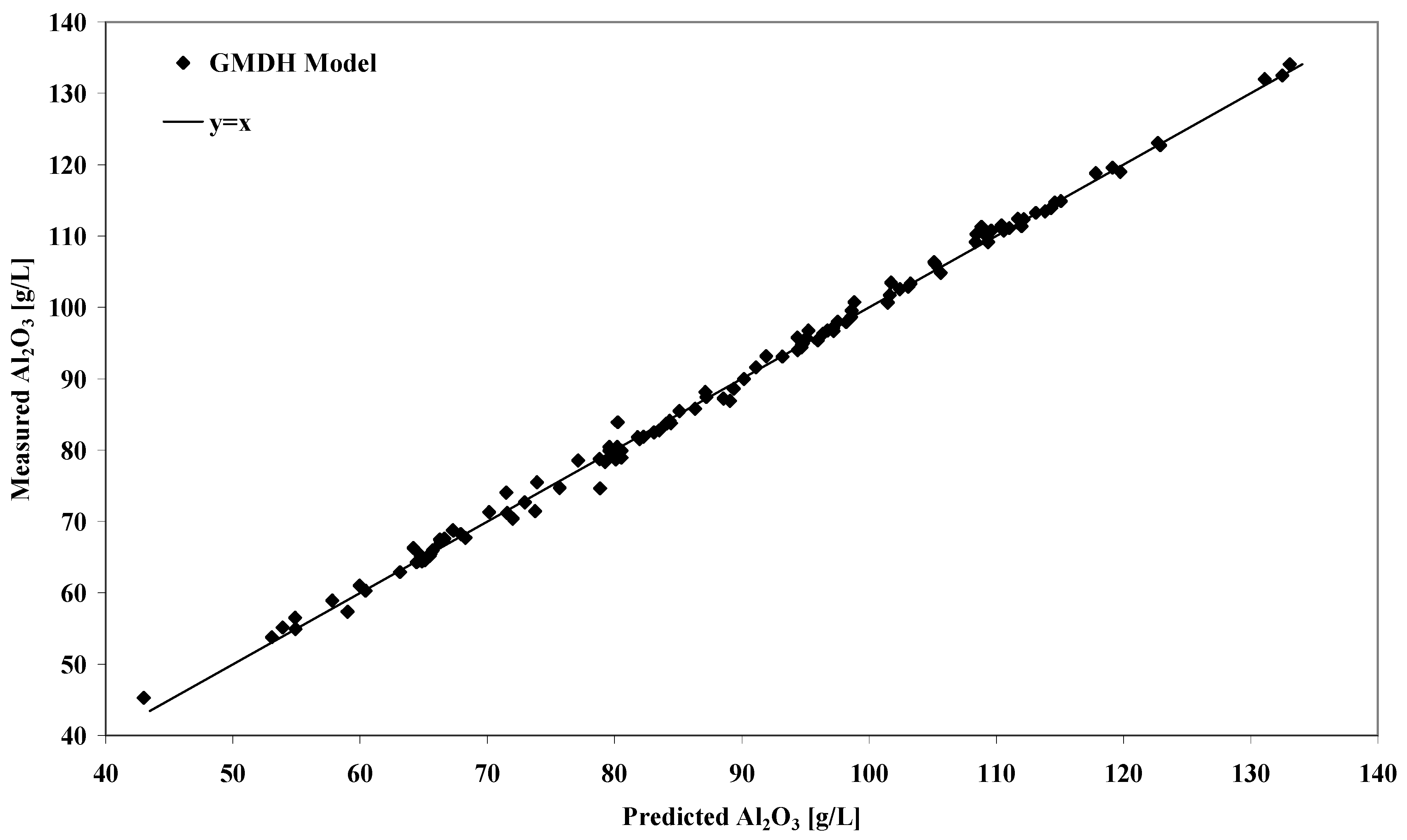
The performance of the GMDH solubility model can be appreciated by inspection of
Figure 1. The linear regression plot of experimental versus modelled equilibrium gibbsite solubility shows that for the entire range of measured data, the model behaves very well. For the 124 solubility measurements covering the ranges outlined in
Table 1, the GMDH model reproduced the experimental values with a
Figure 1.
Plot of predicted versus experimental equilibrium gibbsite solubility concentrations for the model calibration data set.
Figure 1.
Plot of predicted versus experimental equilibrium gibbsite solubility concentrations for the model calibration data set.
Table 1.
Range of liquor constitutions used for the model calibration.Quantities expressed in g/L.
Table 1.
Range of liquor constitutions used for the model calibration.Quantities expressed in g/L.
| Variable | Temp | *C | Na2CO3 | NaCl | Na2SO4 | NaF | **TOC |
|---|
| Range | 55-95 °C | 110 – 160 | 0 – 70 | 0 – 13 | 0 – 4 | 0-7 | 0 – 10 |
mean unsigned error (MUE) of 0.78 g/L Al
2O
3. The corresponding mean signed error (MSE) was -0.17 g/L Al
2O
3 with a standard deviation from the MSE of 1.05 g/L Al
2O
3. The performance of the model can therefore be closely compared with RH’s thermodynamic model which was accurate within a typical error of 1.2 g/L Al
2O
3 at the 95% confidence level [
3].
The GMDH network failed to identify fluoride concentration as a significant variable of the system. This represents a bit of a curiosity. Fluoride is a group 7 element with a high electronegativity and thus, a high propensity of ion formation in an inorganic solvent. If fluoride ions are formed, they should reduce the available solvent for gibbsite dissolution. On the other hand, the binding of F- to Al3+ is unusually strong. It is likely that a considerable fraction of the available fluoride ions are occupied in the form of (OH)3AlF– and associated tetrahedral Al3+ complexes as opposed to free F– ions in solution. Adhering to this argument would explain why fluoride concentration has negligible overall effect on gibbsite solubility.
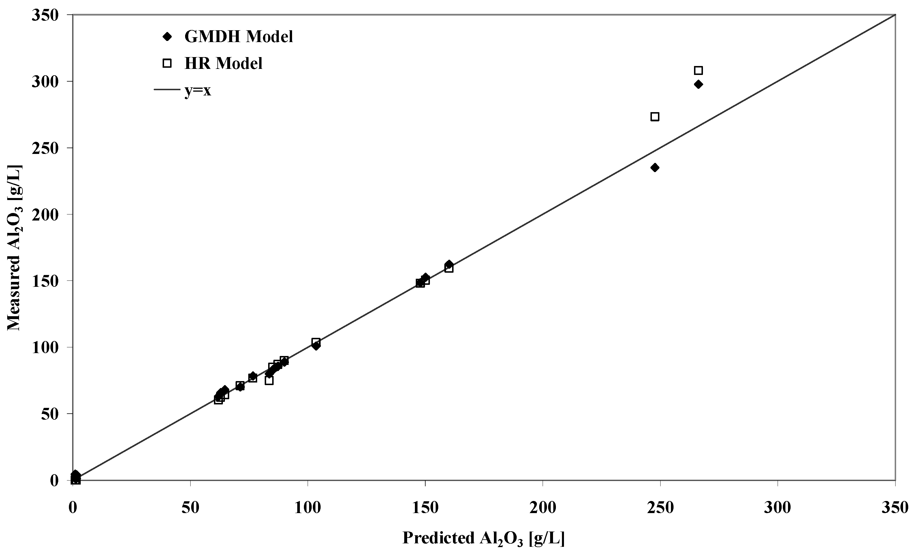
Predicting solubility for conditions outside the range of calibration provides a good test of the reported GMDH model.
Table 2 lists a range of predicted gibbsite solubilities against some previously published results for Worsely liquors fitting this criterion. Despite the possible problems outlined above relating to solution phase speciation, the GMDH model performs very well compared to the experimental results and the RH model predicted values. The strong correlation between the predicted and experimental solubilities is also shown in
Figure 2. It should pointed out that the latter model was calibrated for Worsely liquors so a superior performance should be expected in any case. The analytical quality of the measurements at high and low caustic may be questionable which possibly explains the large deviations at these extremes.
Conclusions
We have demonstrated the successful application of the Group Method of Data Handling to the problem of modelling gibbsite solubility in Bayer process liquors. Using a set of experimentally determined solubility data as input, the GMDH algorithm was able to automatically create a algebraic description of the relationship between equilibrium gibbsite solubility concentration and temperature, caustic concentration as well as impurity concentrations in liquor. This was accomplished with virtually no user intervention. The performance of the final reported model compares favourably with the most sophisticated phenomenological model presented to date which was developed based on the principles of thermodynamics.
Table 2.
Equilibrated liquor conditions and measured gibbsite equilibrium solubilities taken from Ref. 3 compared to predicted values from the GMDH model and Rosenberg and Healy’s thermodynamic model. The associated errors are listed in the final two columns. Concentrations appearing in Italics represent values outside the calibration range (C is caustic expressed as g/L Na2O).
| Equilibrated Liquor Analysis | | Predicted Conc’s |
|---|
| Temp °C | C (g/L) | Na2CO3 (g/L) | NaCl (g/L) | Na2SO4 (g/L) | TOC (g/L) | Measured (g/L) | GMDH (g/L) | HR (g/L) |
|---|
| 80 | 2.4 | 10.0 | 0.0 | 0.0 | 0.0 | 1.6 | 4.10 | 0.09 |
| 60 | 2.5 | 10.0 | 0.0 | 0.0 | 0.0 | 1.0 | 4.53 | 0.05 |
| 80 | 2.5 | 1.1 | 0.0 | 0.0 | 0.0 | 1.5 | 1.33 | 0.02 |
| 60 | 2.7 | 0.3 | 0.0 | 0.0 | 0.0 | 1.2 | 1.07 | 0.01 |
| 175 | 103.6 | 37.2 | 18.79 | 32.82 | 24.96 | 147.9 | 148.5 | 147.9 |
| 175 | 105.0 | 38.3 | 19.97 | 33.25 | 26.19 | 150.1 | 152.6 | 150.3 |
| 85 | 111.0 | 39.4 | 20.1 | 35.1 | 26.7 | 85.2 | 83.2 | 84.9 |
| 85 | 112.5 | 39.9 | 21.3 | 35.46 | 27.94 | 87.4 | 85.7 | 87.1 |
| 65 | 112.7 | 41.4 | 20.1 | 35.87 | 27.28 | 62 | 63.2 | 60.2 |
| 65 | 114.5 | 42.1 | 21.5 | 36.32 | 28.61 | 62.9 | 65.7 | 62.3 |
| 85 | 114.5 | 41.2 | 22.56 | 36.37 | 28.72 | 90.1 | 88.8 | 89.9 |
| 65 | 116.1 | 43.2 | 22.7 | 37.11 | 29.3 | 64.7 | 68.0 | 64.2 |
| 149 | 118.6 | 52.5 | 16.9 | 43.8 | 19.5 | 160.2 | 162.4 | 159.6 |
| 85 | 124.8 | 44.6 | 22.99 | 38.45 | 30.33 | 103.5 | 100.9 | 103.4 |
| 65 | 125.4 | 48.3 | 16.4 | 43.5 | 22.7 | 71.3 | 70.2 | 71.2 |
| 65 | 127.7 | 47.0 | 23.5 | 39.55 | 31.2 | 76.7 | 78.3 | 76.7 |
| 65 | 140.4 | 48.5 | 21.37 | 23.07 | 0.17 | 83.6 | 79.9 | 75.0 |
| 80 | 235.3 | 38.6 | 42.2 | 13.2 | 40.8 | 266.3 | 297.8 | 308.0 |
| 60 | 238.1 | 36.6 | 45.2 | 13.3 | 43.5 | 247.7 | 235.0 | 273.2 |
Figure 2.
Plot of predicted versus experimental equilibrium gibbsite solubility concentrations for liquors conditions outside the range of model calibration.
Figure 2.
Plot of predicted versus experimental equilibrium gibbsite solubility concentrations for liquors conditions outside the range of model calibration.
The predictive behaviour of the model appears to allow for solubility determinations outside of the range of calibration. One very useful feature of the present approach is that the calibration range can easily be extended when new data becomes available. Importantly, the method does not rely on a particular model remaining valid throughout a particular range of data. For example, it is probable that at high caustic concentrations different ion-pairing behaviour occurs in the Bayer liquor than at lower concentrations. A thermodynamic model would have difficulty in describing this type of transition and would require that activity coefficients account for this as a function of caustic concentration. As long as the behavioural transition was smooth, the GMDH algorithm would have the flexibility to adapt itself to include these effects assuming the appropriate experimental data was available.
This manuscript presents a single example of the possibilities offered by GMDH in the field of Industrial Chemistry. There are many situations when a symbolic mathematical model relating input data to some output data is sought where GMDH offers a potential solution. Other obvious Industrial Chemistry and Chemical Engineering applications include, for example, plant process modelling, quantitative structure-activity relationships (QSAR) and quantitative structure-property relationships (QSPR) to name a few.


