Introduction
The interface of computers and chemistry is characterized, among others, by the challenge of predictive toxicology. Quantitative Structure-Activity Relationships (QSAR) are models that attempt to relate chemical structure to biological endpoints such as toxicity. Assuming a common biophysical mechanism, differences in chemical structure for a set of known compounds are mapped to changes in toxicity. The QSAR is then employed to extrapolate to new compounds, on the basis of a tacit assumption which can be expressed in terms of the following equation
where the response R is the magnitude of measured pharmacological/toxicological effect produced by a molecule under
in vitro or
in vivo conditions and p represents either an empirical property or a theoretical parameter for the total molecular structure or relevant substructural fragment(s) [
1]. This paradigm leads to the belief that a proper choice of p will give a precise prediction of R for bioactive molecules. Variable p frequently represents 1) a physical property of molecules or physicochemical substituent constants associated with various functional groups, 2) quantum chemical parameters calculated by different
ab initio or semiempirical methods, or 3) topological indices defined on chemical graphs of molecules using mathematical techniques [
2,
3,
4,
5,
6].
Advantages and disadvantages of empirical and semiempirical QSAR studies are well known. One can argue about difficulties and oversimplifications as well as about advantages and opportunities of structure-activity studies. Questions have been raised about defining relative activities, about separating therapeutic and adverse effects, about obtaining a different outcome for the same drug in different species. Notwithstanding the validity of such concerns and the lack of understanding of underlying mechanisms due to the complexity of biological systems, empirical schemes offer a useful tool to help to filter out from a collection of candidate structures less desirable ones, even if they may not point the most desirable ones [
7]. The graph theoretical approach to be employed here appears capable of resolving some of the above concerns.
A growing area of research in toxicology is the prediction of adverse effects of chemicals by means of QSAR. Indeed, more than one million new compounds are registered per year with the Chemical Abstracts Service. Only few of these chemicals have the experimental data needed for risk assessment. Under these conditions, QSAR estimations can play a key role to fill the gaps and provide information on which compounds may be hazardous and hence essential to be tested. In aquatic toxicology, the QSAR models are generally designed for chemicals presenting the same mode of toxic action [
8].Their proper use provides good simulation results. Problems arise when the mechanism of toxicity of a chemical is not clearly identified. Indeed, in that case, the inappropriate application of a specific QSAR model can lead to a dramatic error in the toxicity estimation [
9]. In order to overcome this drawback, several attempts have been made for proposing methodologies capable to predict modes of toxic action of chemicals in order to select the suitable QSAR models [
10,
11].
In a recent paper, Cronin
et al. [
12] developed a QSAR model based upon the logarithm of the octanol-water partition coefficient and energy of the lowest unoccupied molecular orbital to study the toxicity of aliphatic compounds to the marine bacterium
Vibrio fischeri (
V. fischeri). The aim of this study is to assess the toxicity due to
V. fischeri by means of a particular set of variable topological descriptors, the so called correlation weights of local graph invariants in order to improve previous results.
Toxicity Data
Among the bacterial toxicity essays, the
V. fischeri luminescence inhibition assay is among the more popular. The assay is static in design and offers the possibility of inexpensive assessment of acute toxicity of marine pollutants. Despite the commonplace use of the
V. fischeri assay, the systematic evaluation of electrophilic toxicants with it has yet to be explored fully [
13]. The effects of pollutants on light emission of bioluminescent bacteria was formerly referred to as
Photobacterium phosphoreum and the endpoint is the effective concentration inducing a 50% reduction of bacterial luminescence in a given time of exposure [
14]. The toxicity of aliphatic compounds to the 50% population growth inhibition generally are expressed in mg/l and therefore are converted into log 1/C(mmol/l) for modeling purposes.
The variety of classes of aliphatic compounds is rather representative and it comprises haloalcohols, halonitriles, haloesters, and diones. The complete molecular set is given in
Table 1 together with experimental data and CAS Number. Each of these classes of compounds is thought to elicit toxicity of an electro(nucleo)philic mechanism. This molecular set is identical to that one selected by Cronin
et al. [
12] and this particular choice was made to make a suitable comparison between our results and previous data.
Table 1.
Toxicity data for compounds considered in this study.
Table 1.
Toxicity data for compounds considered in this study.
| Name | CAS Number | log(IGC50-1) |
|---|
| Haloalcohols | | |
| 2-Chloroethanol * | 107-07-3 | -1.42 |
| 2,2,2-Trichloroethanol * | 115-20-8 | -0.46 |
| 1-Chloro-2-propanol * | 127-00-4 | -1.49 |
| 1-Bromo-2-propanol * | 19686-73-8 | -1.19 |
| 6-Chloro-1-hexanol * | 2009-83-8 | -0.27 |
| 8-Chloro-1-octanol ^ | 23144-52-7 | 0.49 |
| 3-Bromo-2,2-dimethyl-1-propanol * | 40894-00-6 | -0.46 |
| 6-Bromo-1-hexanol ^ | 4286-55-9 | 0.01 |
| 8-Bromo-1-octanol ^ | 50816-19-8 | 1.04 |
| 2-Bromoethanol ^ | 540-51-2 | -0.85 |
| 3-Chloro-1-propanol * | 627-30-5 | -1.40 |
| 2,2,2-Tribromoethanol * | 75-80-9 | 0.11 |
| 4-Chloro-1-butanol ^ | 928-51-8 | -0.76 |
| 1,3-Dichloro-2-propanol * | 96-23-1 | -0.79 |
| 3-Chloro-1,2-propanediol * | 96-24-2 | -1.63 |
| Halonitriles | | |
| Chloroacetonitrile * | 107-14-2 | 0.85 |
| 2-Chloropropionitrile ^ | 1617-17-01 | -0.86 |
| 2-Bromopropionitrile * | 19481-82-4 | 0.63 |
| 7-Bromoheptanonitrile ^ | 20965-27-9 | 0.51 |
| 7-Chloroheptanonitrile ^ | 22819-91-6 | 0.29 |
| 3-Bromopropionitrile ^ | 2417-90-5 | -0.50 |
| Dibromoacetonitrile * | 3252-43-5 | 2.40 |
| 4-Bromobutyronitrile * | N/A | -0.47 |
| 5-Bromovaleronitrile ^ | 5414-21-1 | -0.21 |
| 3-Chloropropionitrile * | 542-76-7 | -1.00 |
| 4-Chlorobutyronitrile * | 628-20-6 | -0.93 |
| Bromoesters | | |
| Ethyl-5-bromovalerate ^ | 14660-52-7 | 0.22 |
| 5-Bromopentylacetate * | 15848-22-3 | 0.29 |
| Ethyl-6-bromohexanoate ^ | 25542-62-5 | 0.59 |
| Ethyl-4-bromobutyrate * | 2969-81-5 | -0.03 |
| Ethyl-2-bromopropionate * | 535-11-5 | 1.06 |
| Ethyl-3-bromopropionate * | 539-74-2 | 0.13 |
| Methyl-5-bromovalerate * | 5454-83-1 | -0.08 |
| Ethyl-2-bromoisobutyrate * | 600-00-0 | 0.15 |
| Ethyl-2-bromovalerate * | 615-83-8 | 0.70 |
| Ethyl-2-bromohexanoate * | 615-96-3 | 0.86 |
| DL-methyl-2-bromobutyrate * | 69043-96-5 | 1.02 |
| Diones | | |
| 2,5-Hexanedione * | 110-13-4 | -1.40 |
| 2,4-Pentanedione * | 123-54-6 | -0.27 |
| 2,4-Octanedione * | 14090-87-0 | 0.13 |
| 2,3-Hexanedione * | 3848-24-6 | -0.21 |
| 2,3-Butanedione * | 431-03-8 | -0.23 |
| 3,4-Hexanedione * | 4437-51-8 | -0.01 |
| 2,3-Pentanedione * | 600-14-6 | -0.16 |
| 2,4-Nonanedione * | 6175-23-1 | 0.51 |
| 3,5-Heptanedione * | 724-54-6 | -0.38 |
| 2,3-Heptanedione ^ | 96-04-8 | 0.04 |
| Alkanones | | |
| Acetone * | 67-64-1 | -2.20 |
| 2-Butanone* | 79-93-1 | -1.75 |
| 2-Pentanone ^ | 107-87-9 | -1.22 |
| 2-Decanone * | 693-54-9 | 0.58 |
| 2-Undecanone * | 112-12-9 | 1.50 |
| 2-Tridecanone ^ | 593-08-8 | 2.12 |
| Alkanals | | |
| Butyraldehyde * | 123-72-8 | -0.38 |
| Valeraldehyde * | 110-62-3 | -0.02 |
| Heptaldehyde * | 111-71-7 | 0.00 |
| Octylaldehyde ^ | 124-13-0 | 0.45 |
| Undecylaldehyde * | 112-44-7 | 1.69 |
| Dodecylaldehyde ^ | 112-54-9 | 1.76 |
| Alkenals | | |
| 2-Butenal * | 123-73-9 | 0.70 |
| 2-Pentenal ^ | 1576-87-0 | 0.66 |
| 2-Hexenal * | 6728-26-3 | 0.76 |
| 2-Heptenal * | 18829-55-5 | 1.05 |
| 2-Octenal ^ | 2548-87-0 | 1.20 |
| 2-Nonenal ^ | 18829-56-6 | 1.60 |
| 2-Decenal ^ | 3913-81-3 | 1.85 |
Topological Descriptors
Because the pool of molecular descriptors has increased dramatically during the last decade, the problem of selecting optimal molecular descriptors is a current topic of interest to many researchers [
15]. There are two main procedures to choose optimal molecular descriptors: a) to evaluate thousands of molecular descriptors to find out the best ones and b) to select a few adjustable descriptors and to optimize their variable part. Topological indices are characterized by fixed numerical values, which is independent of the property under consideration. Hence, they can be computed once the bonding pattern or the geometry in the case of 3D structural indices of a molecule are known. However, if we extend the conception of molecular descriptor as a “variable” or “flexible” function depending on some variable part, then we can optimized them for every property considered during the regression analysis. This feature was proposed some time ago [
16,
17] as a novel approach for the characterization of heteroatoms in chemical structures. The search for optimized molecular descriptors has been outline in QSAR [
18,
19,
20,
21], but apparently hay not yet received due attention. The first task when considering optimization of molecular descriptors is to find a generalized form for the descriptor that allows introduction of variables to be optimized.
The optimization of correlation weights of local invariants (OCWLI) is a sort of variable descriptor which has proven to be valuable when applied in QSAR/QSPR analysis [
22,
23,
24,
25]. These studies have been based on local graph invariants of labeled hydrogen-filled graphs (LHFG). The Morgan extended connectivity indices of increasing order have been examined as local LHFG. Another set of local graph invariants were also examined: the path numbers and valence shells proposed originally by Randic [
26]. Paths and walks represent the most elementary graph theoretical concepts. The path of length k, p
k, is defined as a sequence of k consecutive edges of a structure such that no vertex and no edge is repeated in the sequence. The concept is neighbor shells is similar to the concept of paths. The difference is that instead of counting for each atom the number of neighbors at increasing length, one adds the valences of neighbors at increasing separation.
In the present study we resort to OCWLI models based on
- a)
Morgan extended connectivity indices of increasing orders (EC0, EC1, EC2) [
22,
23,
24,
25].
- b)
Path numbers of length 2 and 3 (p
2, p
3) [
26].
- c)
Valence shells of range 2 and 3 (s
2, s
3) [
26].
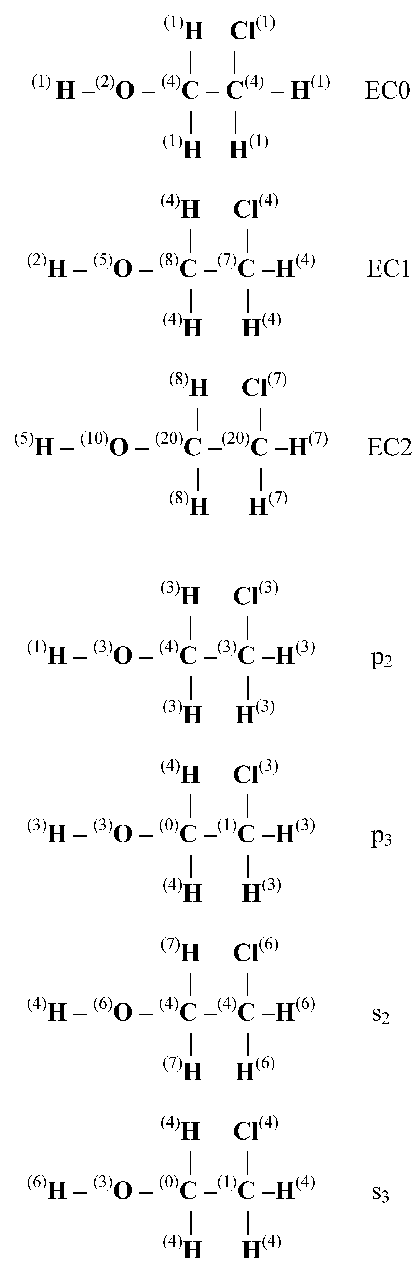
In
Figure 1 we display the numerical values of these invariants for 2-chloro-ethanol.
Figure 1.
Numerical values of LHFG invariants of 2-chloroethanol.
Figure 1.
Numerical values of LHFG invariants of 2-chloroethanol.
Computational Methods
A LHFG is the basis of the present QSAR study. The molecular descriptor is calculated as
where a
k is the chemical element having the k-th vertex of the LHFG, CW(a
k) is the correlation weight of a
k, LI
k is the Morgan extended connectivity index of zero, first and second orders (EC0, EC1, and EC2, respectively) or number path of length 2 and 3 (p
2 and p
3, respectively) starting at the k-th vertex, or valence shell of ranges 2 and 3 (s
2 and s
3, respectively) and CW(LI
k) is the correlation weight of the LI
k. The index n denotes the number of vertices in LHFG.
Evidently, the value of descriptor in Eq.(2) is a function depending on the CW’s. The value of the correlation coefficient between descriptor of Eq.(2) and the activity of interest (in this case log(IGC
50‑1)) is a function of the above-mentioned CW’s. Then, the numerical algorithm is described as follows:
- a)
Resorting to the Monte Carlo method [
18] the values of the CW’s are calculated to yield the largest possible value of the correlation coefficient for a relationship like (1) for the property under consideration and descriptor given by (2). The initial values of the CW’s are taken equal to one.
- b)
Using a least squares method, the following relation is obtained
where a and b are numerical coefficients derived from the fitting procedure and q stands for any of the invariants ECt (t = 0, 1, or 2), p
q, or s
q (q = 1 or 2).
- c)
Finally, the predictive capability of Eq.(3) may be validated from the compounds belonging to the test set.
Computer calculations were carried out with toxicity data taken from Ref. 1 (see
Table 1) and the original molecular set comprising 66 compounds was divided into a training set consisting of 45 molecules and a test set comprising the remaining 21 molecules. We have test several ways for dividing the structures into a training and test set, but final results do not depend significantly on the way to perform such choice, so that we report data for just one of them.
We have analysed linear, quadratic and cubic fitting equations since many correlations, particularly when involving molecules of different size, need not be exclusively linear [
27]. But even if we have molecules of the same or similar size, a quadratic or cubic regression may result in a better description of the relationship than a simple linear model. Construction of linear regression models containing non-linear terms is most often prompted when the data is clearly not well fitted by a linear model, but where regularity in the data suggests that some other model will fit. Non-linear dependency of biological properties on molecular or/and topological parameters became apparent early in the development of QSAR models and a first approach to the solution of these problems involved fitting a parabola in log P [
28].
Results and Discussion
In
Table 2 we have summarized the results of the statistical characteristics of log(IGC
50-1) linear model for training and validation tests obtained by means of the OCWLI based on the previously mentioned LHFG invariants for three different probes. This first step calculation was performed in order to choose the best LHFG invariant/s.
Table 2.
Statistical characteristics of linear OCWLI models of log(IGC50-1) derived from LHFG invariants correlation weighting.
Table 2.
Statistical characteristics of linear OCWLI models of log(IGC50-1) derived from LHFG invariants correlation weighting.
| Invariant | Probe | Training Set (n = 45) | Test Set (n = 21) |
|---|
| | | r2 | s | F | r2 | s | F |
|---|
| EC0 | 1 | 0.6093 | 0.610 | 67 | 0.7212 | 0.558 | 49 |
| 2 | 0.6080 | 0.611 | 67 | 0.7214 | 0.556 | 49 |
| 3 | 0.6079 | 0.611 | 67 | 0.7351 | 0.544 | 53 |
| EC1 | 1 | 0.7517 | 0.486 | 130 | 0.8449 | 0.416 | 104 |
| 2 | 0.7521 | 0.486 | 130 | 0.8452 | 0.418 | 104 |
| 3 | 0.7511 | 0.487 | 130 | 0.8421 | 0.419 | 101 |
| EC2 | 1 | 0.9384 | 0.242 | 655 | 0.8070 | 0.575 | 79 |
| 2 | 0.9406 | 0.238 | 681 | 0.8012 | 0.587 | 77 |
| 3 | 0.9378 | 0.243 | 648 | 0.8041 | 0.575 | 78 |
| p2 | 1 | 0.7253 | 0.511 | 114 | 0.7512 | 0.481 | 57 |
| 2 | 0.6119 | 0.608 | 68 | 0.8272 | 0.472 | 91 |
| 3 | 0.7284 | 0.508 | 115 | 0.7567 | 0.475 | 59 |
| p3 | 1 | 0.7566 | 0.481 | 134 | 0.8132 | 0.422 | 83 |
| 2 | 0.7565 | 0.481 | 134 | 0.8136 | 0.422 | 83 |
| 3 | 0.7567 | 0.481 | 134 | 0.8138 | 0.422 | 83 |
| s2 | 1 | 0.8299 | 0.402 | 210 | 0.8902 | 0.339 | 154 |
| 2 | 0.8303 | 0.402 | 210 | 0.8923 | 0.333 | 157 |
| 3 | 0.8297 | 0.402 | 210 | 0.8903 | 0.334 | 154 |
| s3 | 1 | 0.8231 | 0.410 | 200 | 0.8597 | 0.372 | 116 |
| 2 | 0.8234 | 0.410 | 200 | 0.8587 | 0.377 | 115 |
| 3 | 0.8222 | 0.411 | 199 | 0.8549 | 0.380 | 112 |
A close inspection of numerical data shows that s
2 yields the best prediction.
Table 3 contains numerical values of the correlation weights to calculate the
.
Table 3.
Correlation weights of the LHFG invariants for calculating in the first probe of OCWLI.
Table 3.
Correlation weights of the LHFG invariants for calculating in the first probe of OCWLI.
| LHFG Invariants | Correlation Weights |
|---|
| Chemical elements (ak) | |
| C | 4.185 |
| H | -0.550 |
| Cl | 0.050 |
| O | 1.260 |
| Br | 2.720 |
| N | -0.656 |
| Valence Shell of Second range (s2k) | |
| 0001 | 4.269 |
| 0003 | 2.254 |
| 0004 | 1.674 |
| 0005 | 0.650 |
| 0006 | 0.950 |
| 0007 | 1.117 |
| 0008 | 0.850 |
| 0009 | 0.347 |
| 0010 | 0.662 |
| 0011 | 0.667 |
| 0012 | 0.781 |
| 0013 | 0.850 |
In
Table 4 we present statistical results of linear, quadratic, and cubic fitting equations for training and test sets, respectively, and we also display statistical data for the whole set of 66 molecules.
Table 4.
Statistical results corresponding to linear, quadratic, and cubic regression equations for training and test sets, respectively.
Table 4.
Statistical results corresponding to linear, quadratic, and cubic regression equations for training and test sets, respectively.
| Equation | r2 | s | F |
|---|
| Training set (n = 45) | | | |
| Linear | 0.8299 | 0.4069 | 209.8 |
| Quadratic | 0.8359 | 0.4044 | 106.9 |
| Cubic | 0.8474 | 0.3947 | 75.9 |
| Validation set (n = 21) | | | |
| Linear | 0.8901 | 0.3240 | 154.0 |
| Quadratic | 0.8904 | 0.3325 | 73.1 |
| Cubic | 0.8935 | 0.3372 | 47.6 |
| Complete set (n = 66) | | | |
| Linear | 0.8539 | 0.3802 | 373.9 |
| Quadratic | 0.8573 | 0.3787 | 189.2 |
| Cubic | 0.8627 | 0.3744 | 129.8 |
The analysis of numerical data presented in
Table 4 for training and test sets shows that quite satisfactory results are obtained for predicting toxicity activity. In fact, statistical parameters for the test set are better than those obtained for training set. If one takes into consideration that the first results are genuinely predictive, then it follows plainly the previous assertion. Besides, the relatively high values for regression coefficients make quite reliable the respective predictions for toxicity data of the present molecular set.
The employment of higher polynomial regression equations improves fitting equations, although the amelioration is not very spectacular. However, it seems desirable to resort to this alternative calculation procedure in order to obtain good enough results.
Perhaps the suitable quality criteria to judge present results can be set up through the comparison with other similar theoretical predictions for this molecular set. Cronin
et al reported results on QSAR calculations using selected molecular descriptors to model hydrophobic and electrophilic interactions via log P and E
LUMO parameters, respectively [
12]. In fact, statistical parameters for the whole molecular set (
i.e. 66 molecules) are clearly inferior (n = 66, r
2 = 0.814, s = 0.527, F = 143) with respect to present results (n = 66, r
2 = 0.8627, s = 0.3744 , F = 130, cubic equation,
Table 4).
An alternative manner to organize calculations is to treat each molecular subset separately, as done by Cronin
et al. [
12]. That is to say, the alternative would consist in computing fitting equations for each set of haloalcohols, halonitriles, bromoesters, diones, alkanones, alkanals, and alkenals, respectively. In this case, predictions would improve significantly, as shown in that paper (see equations 1-9 in Ref. 12). We have not resorted to this possibility since the number of molecules within each molecular subset is rather scanty (15, 11, 11, 10, 6, 6, and 7 molecules, respectively), so that final results wouldn’t be statistically significant.
Conclusions
We have shown that OCWLI is a quite suitable tool to model toxicity data for a representative set of aliphatic compounds encompassing a variety of mechanisms of toxic action to Vibrio Fischeri. In fact, fitting equations yield satisfactory predictions for the whole molecular set. In order to judge suitably the degree of accuracy and predictive capabilities of the present model it must be taken into account that we have not removed any outliers to improve final results. Among the molecular descriptors chosen in the present study, the best OCWLI model of toxicity is that one base on the Randic valence shells of second range (i.e. s2). Despite different intimate mechanisms occurring between different chemical compounds comprising the present molecular set, we have gotten a highly predictive, global QSAR.
Another relevant point derived from our calculations is the convenience to employ higher polynomial regression equations to obtain better quantitative predictions. Since it is relatively easy and quite direct to pass from linear to higher order equations, this extra effort does not seem to be very demanding.
Present one parameter QSAR approach to the prediction of toxicity appears to have wide potentiality to a number of species, at separate trophic levels, such as fathead minnow (Pimephales promelas) and Tetrahymena pyriformis. At present, research on this issue is being carried out at our laboratories and results will be published elsewhere in the forthcoming future.

