1 Introduction
Charge transfer (CT) in ion-H
2 collisions is usually described with methods based on the sudden approximation [
1], which is generaly applied for molecular rotation. At low energies, quantal calculations are carried out employing the infinite order sudden approximation (IOSA) (see e.g. [
2]). At higher energies, semiclassical methods are used and the sudden approximation can also be applied for molecular vibration; at sufficiently high energy, the simple Franck-Condon approach is appropriate (see reviews of refs. [
3] and [
4]). A semiclassical treatment with rectilinear trajectories and the sudden approximation for rotation and vibration (SEIKON) has been used in several publications [
5,
6,
7,
8], and the low-
v limit of this approach has been studied in a recent work [
9]. In practice, these calculations require the evaluation of the potential energy surfaces and non-adiabatic couplings for a large set of relative orientations of the H
2 internuclear axis with respect to the ion position vector,
R; this is one reason of the relatively few calculations carried out for ion-molecule collisions.
In recent years, several experiments [
10,
11] have studied the dissociation of molecules after collision with ions as a function of the molecular orientation. Nevertheless, the main results of ion-molecule beam experiments are orientation-averaged cross sections (OACS); in fact, these are the only results available for single electron capture processes in ion-H
2 collisions. The calculation of OACS requires an extensive calculation of molecular data, as well as a cumbersome 2D interpo-lation of potential energy surfaces and dynamical couplings. For H
2 collisions with multicharged ions, CT takes place via non-adiabatic transitions at relatively large internuclear distances, where anisotropy effects are unimportant and, a simplified isotropic approximation is appropriate. In this approximation, energies and couplings are taken to be independent of the orientation of the H
2 internuclear axis. The situation is different for singly charged ions-H
2 collisions; in this case, transitions leading to CT occur at short
R. We consider in this paper H
++H
2 collisions, which are the benchmark of these reactions, and are otherwise important in tokamak divertor plasmas (see [
12,
13] and references cited therein). Early semiclassical calculations of ref. [
14] reported a sizeable anisotropy effect on H
++H
2 CT cross sections, but the validity of this conclusion is limited by the Franck-Condon approximation employed to evaluate the vibronic dynamical couplings.
In ref. [
7] it was shown that anisotropy effects on dinamical couplings are less important for H
++H
2 than for Li
++H
2 at energies
E > 0
.1 keV; results for Li
++H
2 collisions [
7] pointed out large differences between cross sections calculated using the isotropic approximation for different orientations, and between them and the OACS. However, it was also shown that an average of isotropic results yields cross sections in good agreement with the OACS. This finding, which implies a significant simplification of the computation, has not been checked for other systems. Moreover, the isotropic approximation is the basis of IOSA treatments, where calculations for fixed molecular orientation are carried out, followed by an average of the ensuing cross sections; this is the method employed in IOSA treatments of CT in H
++H
2 [
15,
13].
As concluded in ref. [
9], for H
++H
2 at
E < 0
.1 keV, a calculation beyond the sudden vibrational approximation is required. The first aim of the present work is to study anisotropy effects in this energy range. We perform an eikonal vibronic close-coupling calculation, similar to that employed in [
9], using the diatomics in molecules (DIM) potentials [
16] because, as in refs. [
17,
14,
15,
18,
13], it allows the evaluation of energies and interactions along each trajectory without using 2D interpolation, which is very useful when many orientations are considered. Although the DIM aproximation limits the precission of our results, the aim of the present paper is to study anisotropy effects rather than obtaining very precise cross sections.
The paper is organized as follows: In
section 2 we explain the semiclassical vibronic close-coupling method employed, the use of DIM wavefunctions, and the calculation of OACS. In
section 3 we present our main results, and discuss the use of simplified methods to evaluate OACS. Our conclusions are summarized in
section 4. Atomic units are used unless otherwise stated.
3 Results
The Hamiltonian matrix elements in the vibronic basis can be expressed as:
where
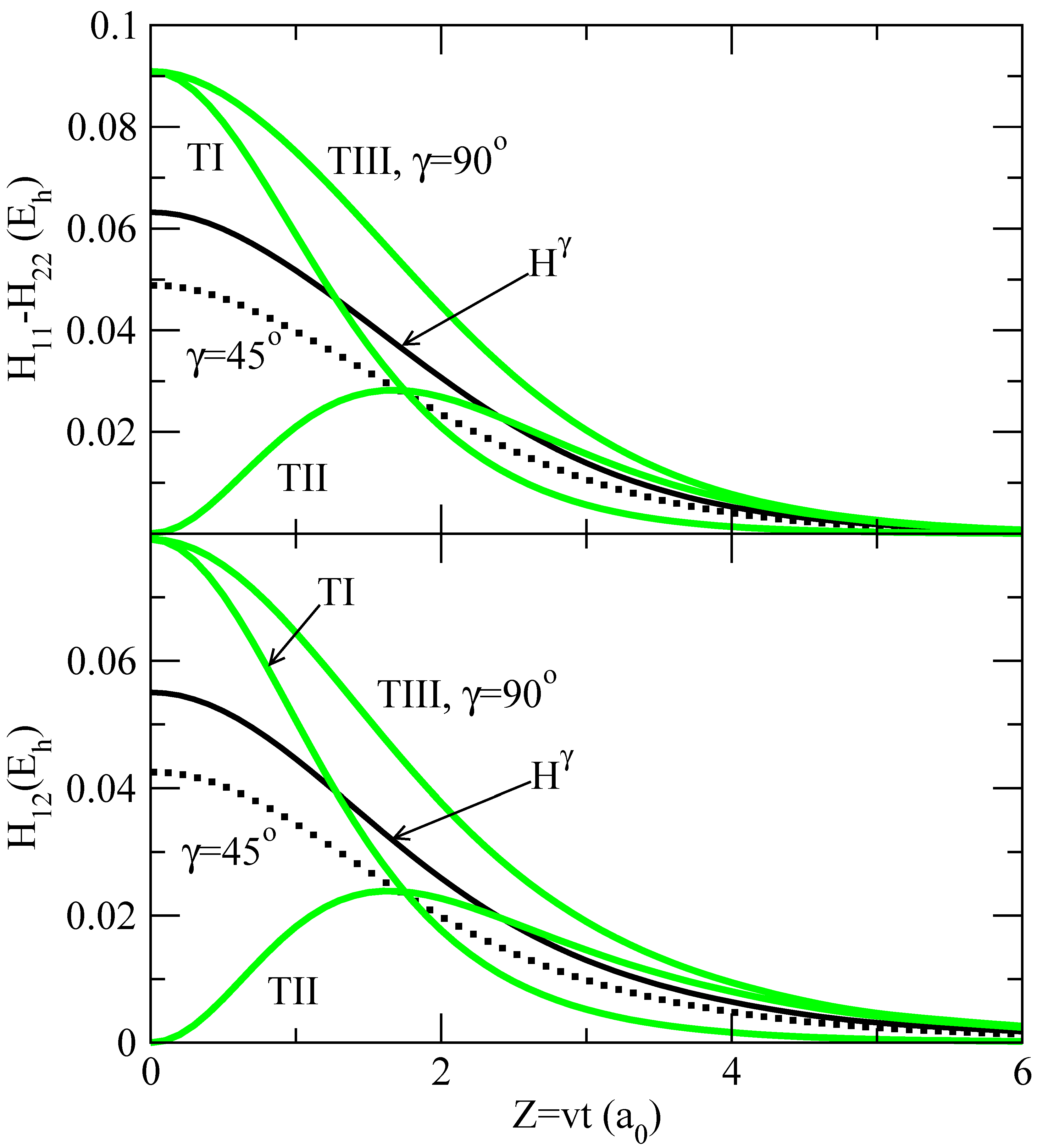
The orientation dependence of the couplings of eq. (13) is therefore a consequence of the dependence of the electronic matrix elements
Hjk of eq. (27), which is illustrated in
figure 2. There, we have plotted the values of
H22 − H11 and
H12 along a representative trajectory with
b = 1
.75 a
0, and for
t > 0. In the top panel of
figure 2, we show the values of the differences: [
H22 − H11](
R,γ = 90°) and [
H22 − H11](
R,γ = 45°), while the bottom panel contains
H12(
R,γ = 90°) and
H12(
R,γ = 45°). In both cases, to make the illustration more clear, we have subtracted from these couplings the corresponding values for
γ = 0. It can be noted that the dependence of the matrix elements
Hjk on
γ is almost linear. We have also included in
figure 2 the orientation averaged couplings
As a consequence of the quasi-linear dependence of
Hij on
γ, these average values are close to the matrix elements evaluated at
γ = 57.3° ≃ 60°, obtained for a linear function
Hij (
γ).
In
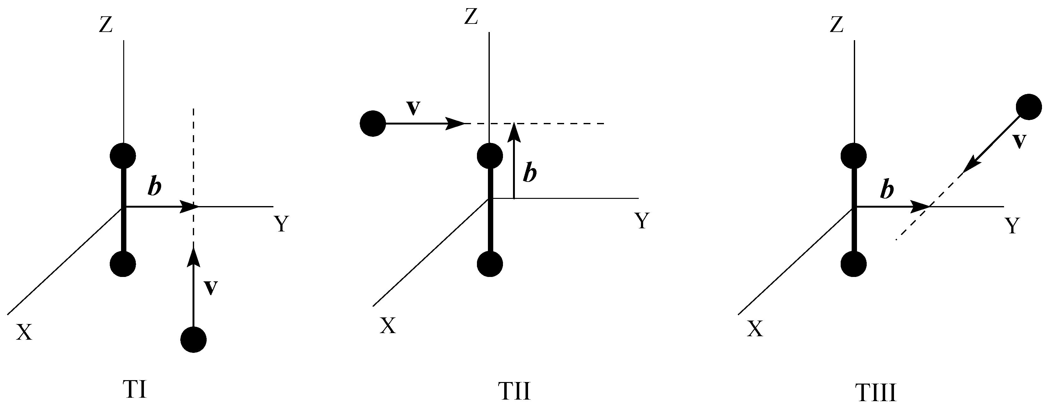
fig. 2, we also include the values of the matrix elements as functions of
Z =
vt for trajectories I, II and III. From the definition of trajectory III (see also
fig. 1), the angle
γ ≡ 90° along this trajectory, which leads to couplings identical to the isotropic ones for this value of
γ. Couplings along trajectory I join smoothly the isotropic values for
γ = 90° at
t = 0 with those for
γ = 0° at
t → ∞, while the inverse situation holds for trajectory II: the values for
γ = 0° are reached at
t = 0 and those for
γ = 90° for
t → ∞. From
fig. 2, we can also note that the orientation dependence of the couplings is very small at large internuclear distances; as a rule, we can neglect the anisotropy for
Z > 4 a
0 (
R > 4
.4 a
0)
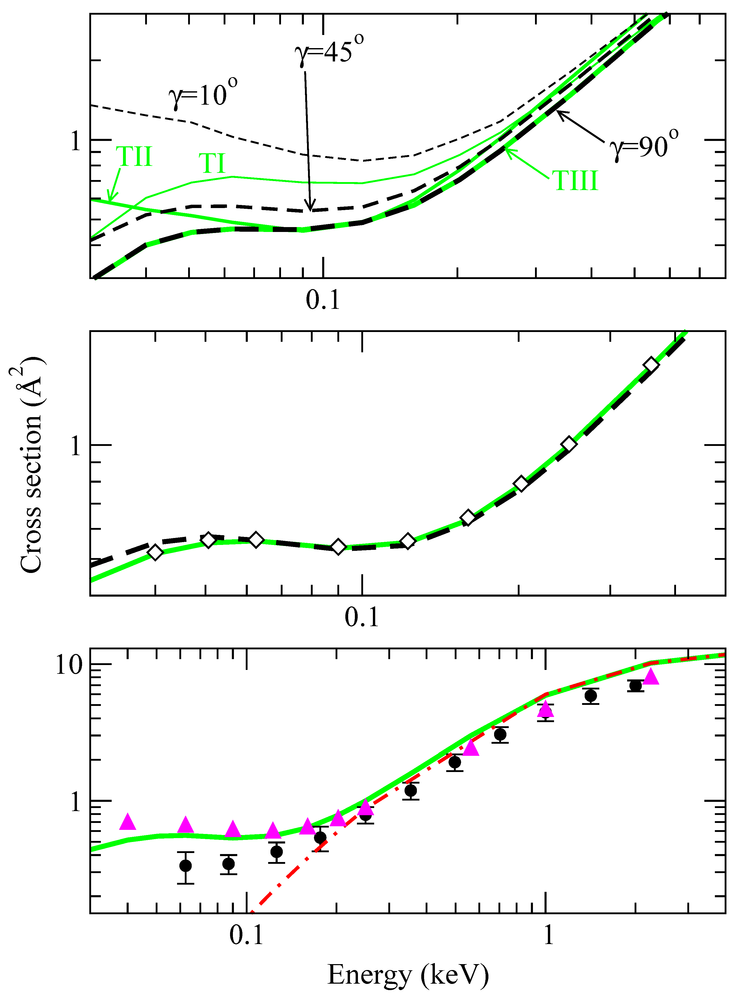
Integration of the system of differential tial equations (13) in the isotropic approximation yields the CT cross sections
(
v,γ0) (see the top panel in
fig. 3); these cross sections do not appreciably depend on
γ0 for
E > 0
.2 keV (differences are of about 10%), in agreement with the conclusions of ref. [
7], but the dependence increases as
E decreases:
(
v, γ0 = 10°) is a factor of 5 larger than
(
v, γ0 = 90°) at
E ≃ 40 eV. We have also included in
fig. 3 the values of
, which exhibit smaller differences than the isotropic ones (at most a factor of 2 between
σII and
σIII at
E = 0
.05 keV). As a first result of the present calculation, the anisotropy of the couplings leads to a significant orientation dependence of total CT cross sections.
Figure 2.
Hamiltonian matrix elements Hij(R, γ) as functions of Z(= vt = ) for several values of γ and with γ(t) for trajectories I, II and III. The full lines labelled as Hγ are the average couplings from eq. (28). Top panel: values of [H22 − H11](R, γ) − [H22 − H11](R,γ = 0). Bottom panel: values of H12(R, γ) − H12(R, γ = 0).
The OACS obtained using eq. (21) and the simplified methods of eqs. (24) are plotted in the middle panel of
fig. 3. It can be noted that the results of averaging over trajectories (eq. (21)) or averaging the isotropic cross sections (eq. (24)) are practically indistinguishable, and the small differences at low
v are probably due to the simple six-trajectory expression used to perform the trajectory average. There is a very good agreement between the OACS and the isotropic result with
γ0 = 45°, which is repeated in the middle panel (with diamonds) for clarity. This indicates that the calculation of
(
v,γ0) provides a good approximation to
when an intermediate
γ0 is employed, such that the coupling matrix
H fulfills
H(
R, γ0) ≃
(
R) (see eq. (28)). This supports our
ab initio results of ref. [
9], obtained with
γ0 = 45°.
In the bottom panel of
fig. 3, we compare the present OACS with the experimental values of ref. [
21]. We have also included in this figure the SEIKON values obtained with DIM potentials and fixed
γ0 = 45° and the vibronic close coupling result calculated with
ab initio energies and couplings and fixed orientation
γ0 = 45°. By comparing the present averaged results, which are practically identical to the isotropic ones obtaned at
γ0 = 45°, with the
ab initio ones, we obtain that the errors introduced in the total cross section by the DIM approximation are smaller than 25%. The comparison with the SEIKON calculation confirms the result of ref. [
7] of a small orientation dependence in the energy range where the SEIKON method is valid.
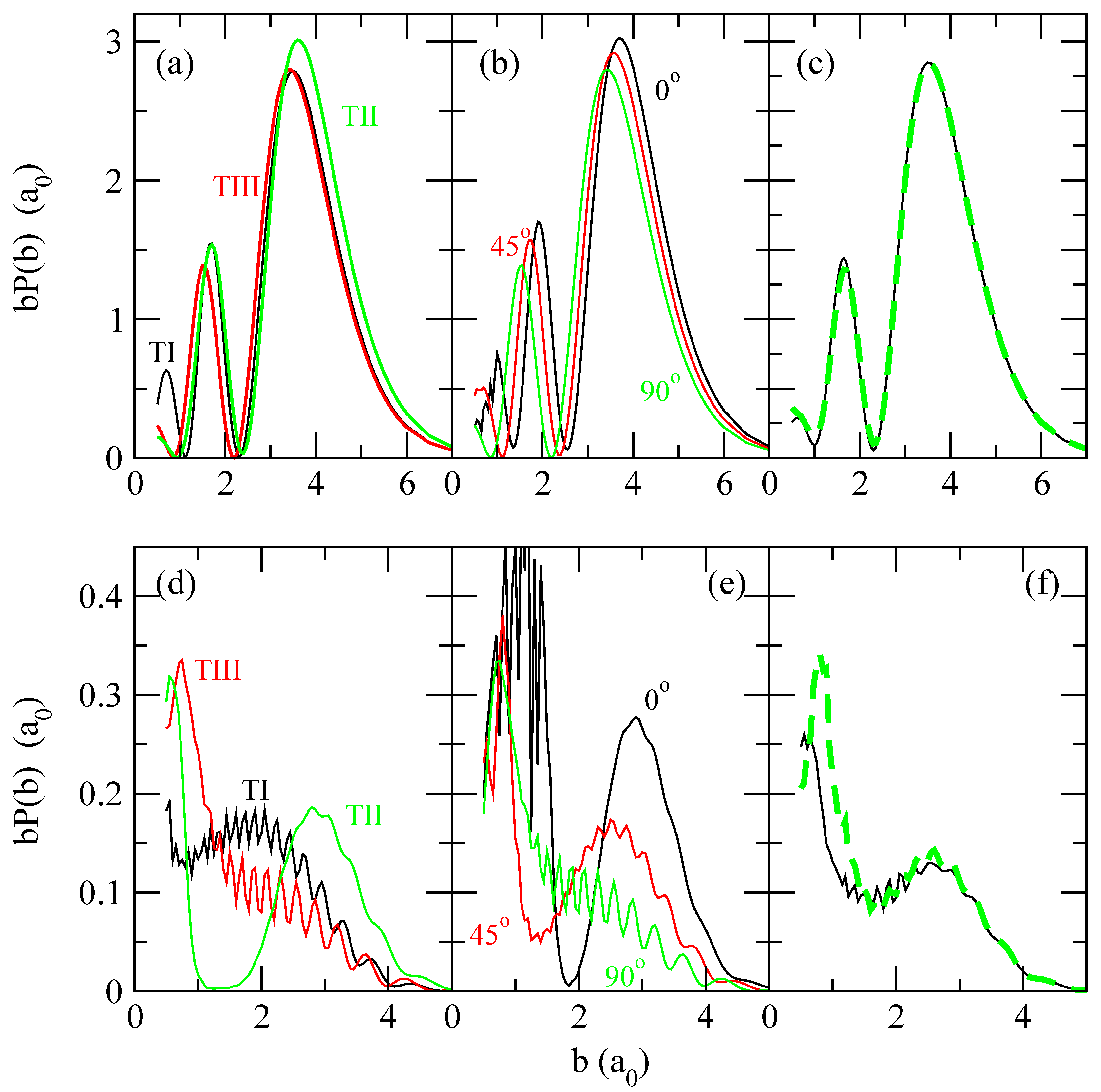
To analyze the results of
fig. 3, we have plotted in
fig. 4 the values of transition probabilities
bPct(
b) and b
(
b) for two impact energies (4 keV and 62.5 eV). At
E = 4 keV, the shapes of all curves in
fig. 3 are very similar in all calculations, showing a broad maximum for
b > 3 a
0, where the couplings are practically independent of
γ (see
fig. 2). When
v decreases, the importance of trajectories with small
b increases leading to a larger anisotropy of the transition probabilities. The comparison of
bPct(
b) of trajectory II with those of trajectories I and III at
b > 2.0 a
0 and
E = 62.5 eV shows a shift of the former to larger
b. To explain this shift (see also ref. [
22]), we assume that, at relatively large
b, the interaction matrix elements are dominated by the interaction of the incident H
+ ion with the nearest H atom of H
2, and a given distance from H
+ to the nearest H nucleus is reached at larger
b in trajectory II than in I and III (see
fig. 1). At low
b, the interaction between the incident ion and both H atoms are equally important, yielding different shapes of the three curves in
fig. 3(d). By comparing the transition probabilities for trajectories I and II in
fig. 3(d) with those calculated using the isotropic approximation (
fig. 3(e)), and other intermediate values of
γ0 not shown in the figure, it can be seen that the former calculation cannot be simplified by taking a constant value of
γ along these trajectories, while, as mentioned before, for trajectory III
γ ≡ π/2. However, a good agreement is found between the averages shown in the third panel of
fig. 4, which explains the good agreement between the OACS of
fig. 3 as due to a compensation of differences between the isotropic calculations. The possibility of using a single isotropic calculation to evaluate orientation averaged transition probabilities is checked
Figure 3.
Charge transfer cross sections calculated using different approximations. Top panel: comparison between cross sections obtained for three characteristic trajectories (grey lines,
,
and
with those obtained with the isotropic approximation at three angles (dashed lines,
(
γ0 = 10°),
(
γ0 = 45°) and
(
γ0 = 90°)), as labeled in the figure. Middle panel: comparison between cross sections averaged over trajectories,
σct (eq. (21), grey solid line), with those averaged over isotropic results,
(eq. (24), dashed line), and with the isotropic result at
γ0 = 45° (◇). Bottom panel: comparison between the trajectory average of the middle panel (grey solid line) with an isotropic calculation at
γ0 = 45° using
ab initio couplings and potentials (solid triangles), a SEIKON calculation with DIM couplings and potentials at
γ0 = 45° (dashed-dotted line) and the experimental results of [
21]. Note the different scales in the panels.
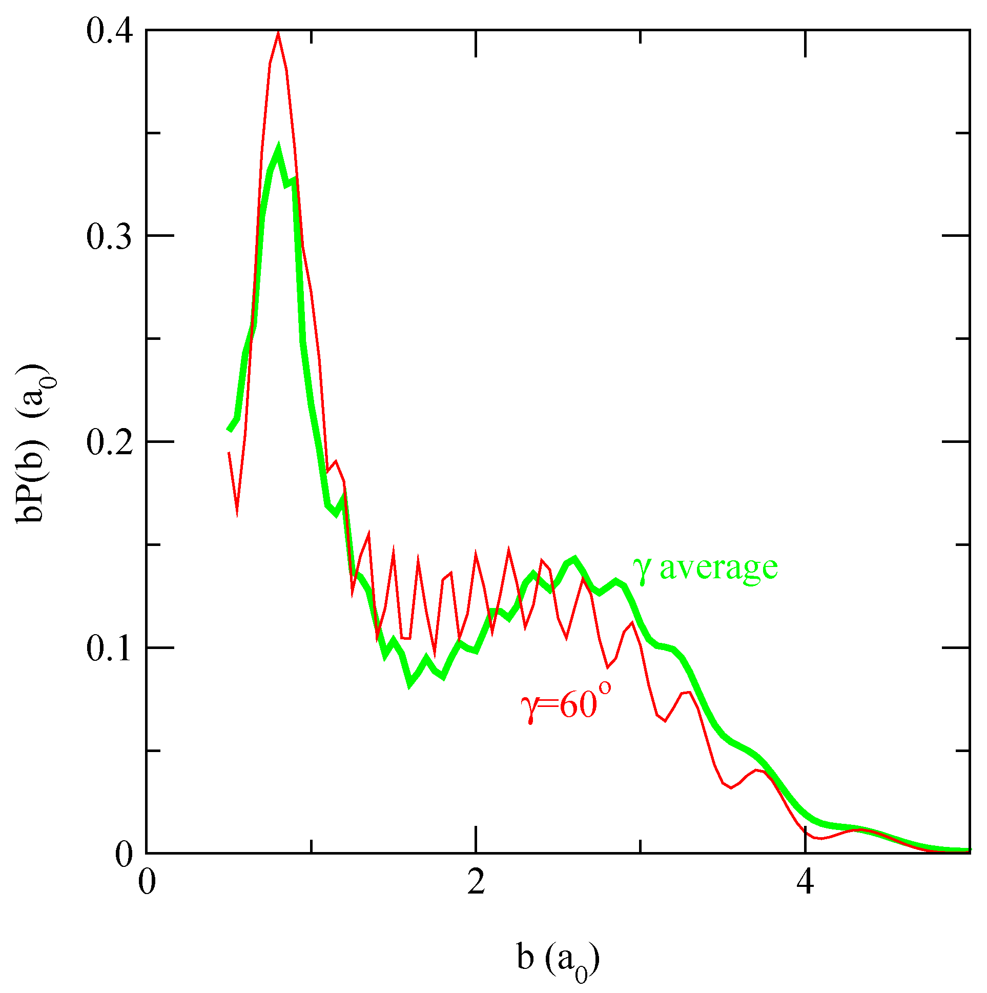
in
fig. 5. We find that
b(
b;
γ0 = 60°), which is very close to the probability obtained with the average interaction matrix, approximately reproduces the shape of the orientation averaged transition probabilities.
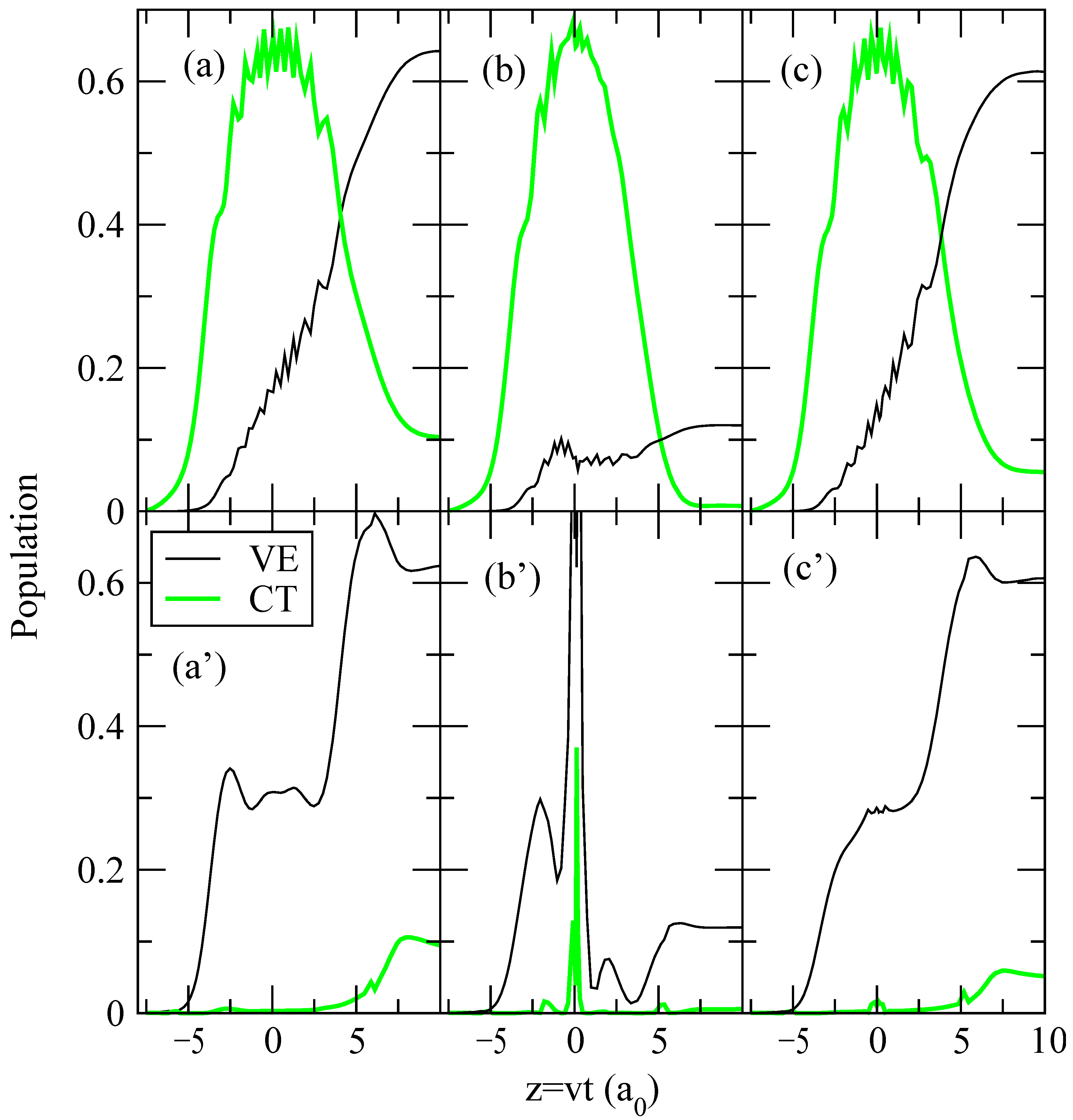
A more detailed information on the origin of the differences between transition probabilities for trajectories I, II and III is obtained from the “collision histories”, which are the time evolution of the populations |
ajν|
2 of the vibronic states (see eq. (12)). To relate these populations with the adiabatic CT mechanism at low
v, described in [
9], the collision histories for
b = 1.75 a
0 and
E = 62.5 eV are plotted in
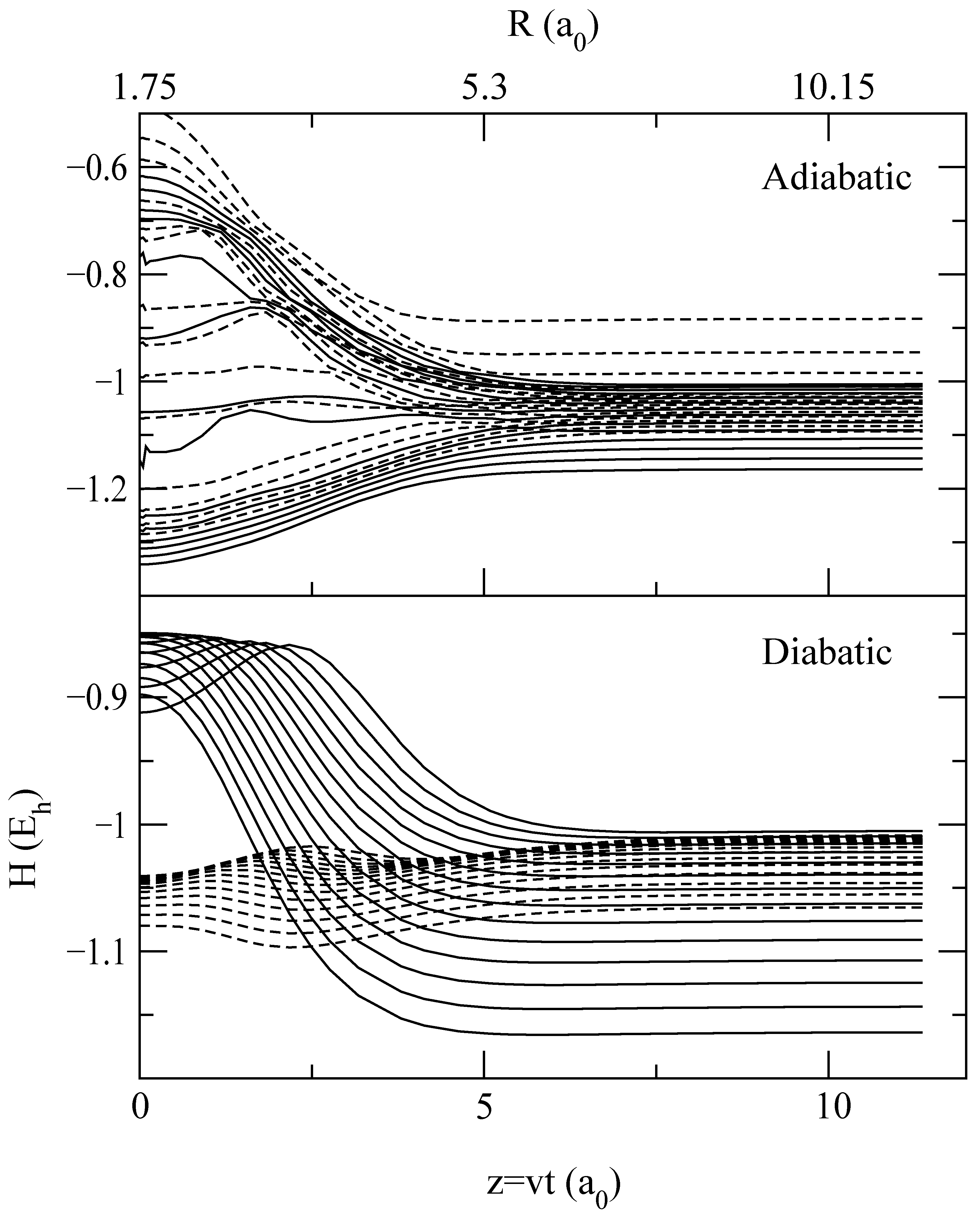
fig. 6 in diabatic and adiabatic bases (see eq. (16)), and to help to understand them, the energy correlation diagrams in both bases are shown in
fig. 7 and
fig. 8 for trajectories I and II respectively. In this respect, it is interesting to note the large differences between adiabatic and diabatic correlation diagrams. This indicates that the interaction matrix elements in the latter are very strong, which makes difficult to understand the mechanism in this basis; e.g. the crossings are not traversed quasi diabatically.
The mechanism for trajectories I and III, in the diabatic representation, involves strong transitions from the entrance channel to the charge transfer ones for
t < 0 through the series of crossings. This gives rise to the oscillations shown in the total charge transfer population of
fig. 6. For
t > 0, the population is transferred back from the charge transfer states to the entrance channel and the excited vibrational states of H
2. The mechanism in the adiabatic basis is rather different: the first steps, at
t < 0, are transitions from the entrance channel to the first excitation channels at
R < 5 a
0, where the relevant energy surfaces approach. In this basis, CT takes place at
t > 0 through transitions from excited vibrational states of H
2 to the charge transfer ones, because they are quasi degenerate; this is the mechanism described in [
9] and first suggested in the trajectory surface hopping study of ref. [
23].
The mechanism for trajectory II (
figure 6(b,b’)) looks very different of those for the other trajectories. However, the differences are mainly due to the shift effect to larger
b values of
bPct(
b) mentioned above: for the particular value of
b (1.75 a
0) of
fig. 6, and using the adiabatic representation, the transitions near
Z = 0 in trajectory II take place in a series of narrow avoided crossings, which are reached in trajectories I and III at lower
b. A common characteristic of the illustrations shown in
fig. 6 is that the non-adiabatic transitions take place over a wide time interval, which implies a wide range of values
γ, in trajectories I and II, leading to the inaccuracy of using a simplified treatment with couplings calculated for a single
γ to evaluate the corresponding transition probabilities.
Figure 4.
Charge transfer transition probabilities for E = 4 keV (panels (a,b,c)) and E = 62.5 eV (panels (d,e,f)). Panels (a) and (d): bPct(b) for trajectories I, II y III, as indicated in the figure. Panels (b) and (e): b(b; γ0 = 60°) for γ0 = 0°, 45°, 90°, as indicated in the figure. Panels (c) and (f): Average of transition probabilities obtained with the isotropic approximation for several values of γ0 (dashed-thick lines) b(b) (eq. (25)); average of transition probabilities obtained for trajectories I, II and III (solid-thin line) bPct(b) (eq. (20)).
Figure 5.
Comparison between the charge transfer transition probabilities averaged over γ
0 of
Figure 4, panel (f), (grey thick line) with a single isotopic result at γ
0 = 60° (thin line) at E = 62.5 eV.
Figure 5.
Comparison between the charge transfer transition probabilities averaged over γ
0 of
Figure 4, panel (f), (grey thick line) with a single isotopic result at γ
0 = 60° (thin line) at E = 62.5 eV.
4 Conclusions
The calculations of the present work focus on the effect of the anisotropy of the interaction potential on charge transfer cross sections in H
++H
2(X
1,
ν = 0) collisions, as a benchmark case of ion-diatomic molecule collisions. In the calculation we have employed commonly-used DIM electronic wave functions. At high impact energies,
E > 200 eV, this process takes place [
9] through direct transitions from the entrance channel to the CT ones, which are accurately described by means of a sudden vibrational approach. We have shown that, at these energies, total CT cross sections arise as a consequence of transitions at relatively large impact parameters, and therefore large H
++H
2 distances, where coupling matrix elements are practically independent of the angle
γ between vectors
R and
ρ. For
E < 200 eV, a resonant mechanism becomes important; this involves transitions from excited H
2 vibrational states, populated at short
R, to quasi-degenerate CT channels. Since this latter mechanism involves transitions at short
R, anisotropy effects become more important at low
v. In order to describe the resonant mechanism, it is indispensable [
9] to use a vibronic close-coupling basis, and our method is based on this formalism.
A first set of results of the present calculation includes cross sections calculated for trajectories
Figure 6.
Collision histories of vibrational excitation (VE) and charge transfer (CT) channels for trajectories I (a,a’), II (b,b’) and III (c,c’). Collision energy is E = 62.5 eV and impact parameter b = 1.75 a0. Panels (a,b,c) contains results in the diabatic basis, while panels (a’,b’,c’) are in the adiabatic basis.
Figure 7.
Energies of vibronic adiabatic (top panel) and diabatic (bottom panel) states as functions of the nuclear coordinate Z = vt for the trajectory I with b = 1.75 a0. Solid lines correspond to elastic and H2 vibrational excitation channels and dashed lines to charge transfer channels.
Figure 7.
Energies of vibronic adiabatic (top panel) and diabatic (bottom panel) states as functions of the nuclear coordinate Z = vt for the trajectory I with b = 1.75 a0. Solid lines correspond to elastic and H2 vibrational excitation channels and dashed lines to charge transfer channels.
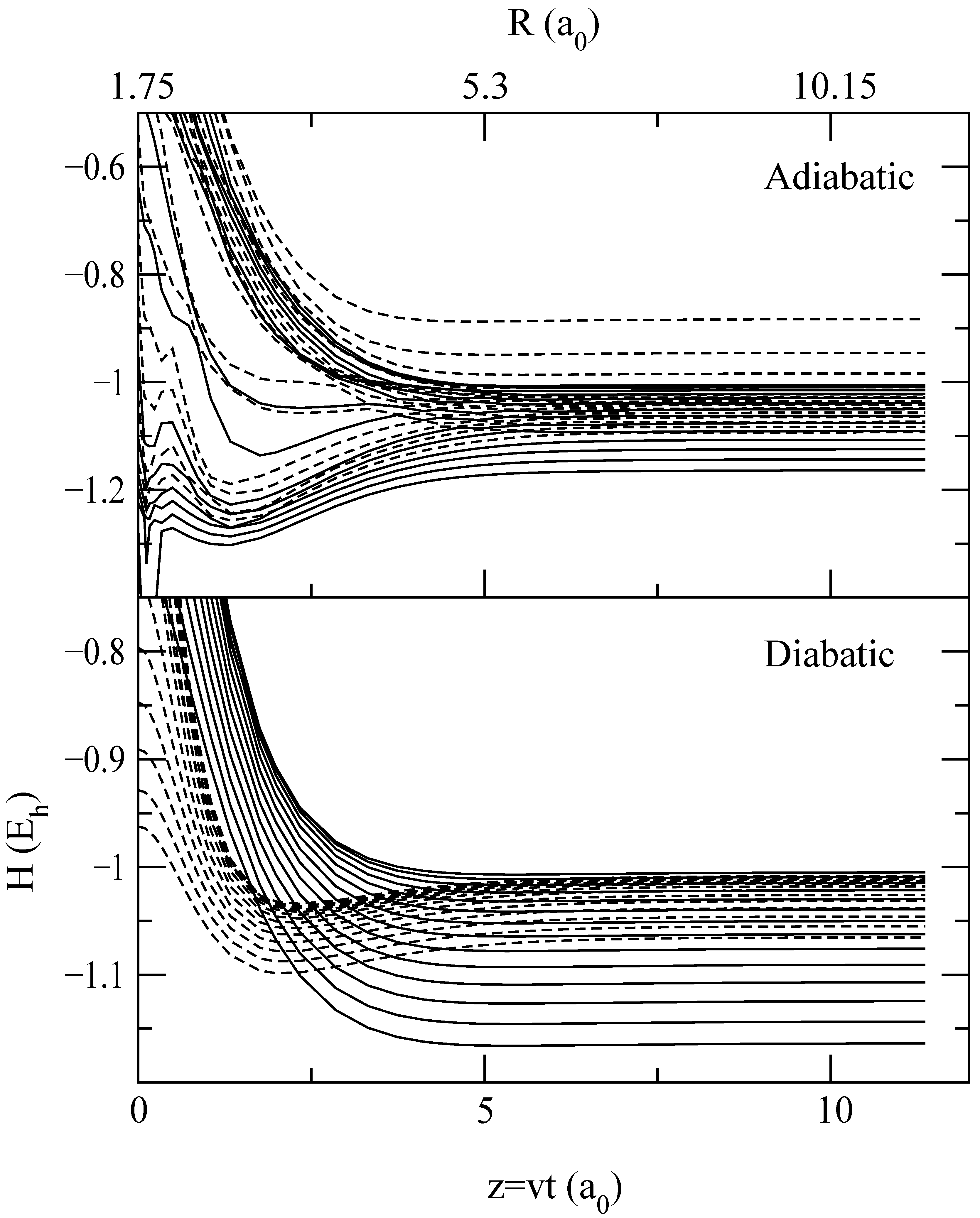
Figure 8.
Same as
fig. 7, but for trajectory II
Figure 8.
Same as
fig. 7, but for trajectory II
where the H
2 orientations with respect to the ion velocity are kept fixed , but
γ changes during the collisions. In particular, we have considered the three trajectories of
fig. 1; these calculations are directly relevant to possible orientation dependent experiments such as those reported in refs. [
10,
11]. Our results at energies
E < 200 eV show that, for this system, CT transition probabilities and cross sections cannot be obtained by assuming that transitions take place at a single value of
γ, but an interval of angles are important, and this is the origin of the differences found between the calculated cross sections for the three trajectories. Besides, although this orientation dependence is a consequence of the anisotropy of the electronic Hamiltonian matrix elements, its influence on the final results is conditioned by the mechanism of the process in the vibronic basis. This is clear from the mechanisms discussed in
fig. 6, with transitions taking place in the crossing regions of
fig. 7, which do not have a counterpart in the electronic Hamiltonian matrix elements of
fig. 2.
The second point considered in this work refers to the calculation of OACS, which are the most common output of experiments. Since the evaluation of OACS requires the calculation of potential energy surfaces and couplings as functions of the three parameters R, ρ and γ, involving in general a considerable computational effort, it is useful to check on approximate methods to evaluate OACS. In this respect, we have considered an isotropic approximation where γ(t) is taken equal to a constant γ0. Such an isotropic calculation of CT cross sections has been carried out for γ0 = 45° with both DIM and ab initio couplings, yielding errors much smaller than the variation of DIM cross sections with γ0, which support the usefulness of the DIM method to study anisotropy effects. Our main conclusions on this second point are: 1) The CT cross sections averaged over trajectories are practically identical to the average over γ0 of cross sections from isotropic calculations. 2) The average of cross sections agrees with the cross section calculated with a Hamiltonian matrix averaged over γ that corresponds to a value of γ0 ≃ 60°. 3) Small differences are found between CT cross sections from isotropic calculations with γ0 in the range 4°–60°. These results are encouraging in order to simplify the calculation, but further work is required, since the agreement between cross sections seems to be due to cancellations in the average procedure of differences between transition probabilities for different γ0 or different trajectory orientations. However, it is expected that the CT reaction in H++H2 presents comparatively larger anisotropy than collisions involving multicharged ions, where transitions occur at large R, and because the special CT resonant mechanism at low v increases the importance of transitions at short R in CT cross sections.
