Electricity Consumption Forecasting Scheme via Improved LSSVM with Maximum Correntropy Criterion


School of Automation and Information Engineering, Xi’an University of Technology, Xi’an 710048, China
*
Author to whom correspondence should be addressed.
†
Current address: Department of Electrical Engineering, Xi’an University of Technology, Xi’an 710048, China.
‡
These authors contributed equally to this work.
Entropy 2018, 20(2), 112; https://doi.org/10.3390/e20020112
Submission received: 15 November 2017
/
Revised: 11 January 2018
/
Accepted: 5 February 2018
/
Published: 8 February 2018
(This article belongs to the Special Issue Entropy in Signal Analysis)
Abstract
:In recent years, with the deepening of China’s electricity sales side reform and electricity market opening up gradually, the forecasting of electricity consumption (FoEC) becomes an extremely important technique for the electricity market. At present, how to forecast the electricity accurately and make an evaluation of results scientifically are still key research topics. In this paper, we propose a novel prediction scheme based on the least-square support vector machine (LSSVM) model with a maximum correntropy criterion (MCC) to forecast the electricity consumption (EC). Firstly, the electricity characteristics of various industries are analyzed to determine the factors that mainly affect the changes in electricity, such as the gross domestic product (GDP), temperature, and so on. Secondly, according to the statistics of the status quo of the small sample data, the LSSVM model is employed as the prediction model. In order to optimize the parameters of the LSSVM model, we further use the local similarity function MCC as the evaluation criterion. Thirdly, we employ the K-fold cross-validation and grid searching methods to improve the learning ability. In the experiments, we have used the EC data of Shaanxi Province in China to evaluate the proposed prediction scheme, and the results show that the proposed prediction scheme outperforms the method based on the traditional LSSVM model.
1. Introduction
With rapid socioeconomic development and the improvement in living standards of residents, the liberalization of the sales side has become an important part of the electricity reform. Electricity selling enterprises have formed a new trading platform and profit model based on the power supply and distribution service. However, the user’s electricity consumption (EC) is easily affected by many factors and shows clear volatility. Therefore, it is necessary for electricity selling companies to make reasonable electricity forecasting systems. For the current bilateral bidding system, electricity selling enterprises buying more or less electricity will face unnecessary economic losses; thus the accuracy requests of electricity demand forecasting are increasingly high.
At present, the methods for electricity consumption prediction (ECPM) can essentially be classified into two types: the traditional prediction method and the intelligent prediction method. In [1], a correction was introduced to correct the coefficients of the Non-homogenous discrete exponential Grey Model (NGM) model, and the raw data was processed with the buffer operator. Finally, a gray prediction model with optimized coefficients was established. However, this model does not consider some of the effects of other factors for electricity. Xue et al. [2] proposed a method of quantifying stochastic change, and its quantized value as a predictive model was used for influencing factors of monthly EC. In addition, the impact of stochastic changes on the monthly sales of electricity was considered reasonable, and thus the model prediction accuracy was effectively improved. An improved support vector regression algorithm was proposed by using the seasonal index adjustment strategy to fine-tune the model prediction error and optimize the key parameters on the basis of the fruit fly algorithm in [3]. A short-term prediction model of building energy consumption based on artificial neural networks (ANNs) and a Bayesian regularization algorithm was developed in [4], and the influence of the parameters such as the delay and the number of hidden neurons was discussed carefully. In addition to the conventional factors such as temperature, the heat island effect as an unconventional factor has also been considered in [5,6,7,8] to improve the accuracy of the prediction. Although these methods above perform well, the following problems should be considered further: (1) Good prediction results mostly depend on a large amount of historical electricity data; however, most users cannot provide enough data; (2) The assumption of the prediction error with a Gaussian distribution is usually used in most of the intelligent algorithms, but it is inconsistent with the diversity of true prediction errors; (3) The prediction results are easily influenced by the type and characteristics of the data.
In order to address these problems, the least-square support vector machine (LSSVM)-based prediction model [9] is introduced to solve the problem of too few data samples effectively. At the same time, the mean square error (MSE) is used as a risk function in the LSSVM model to evaluate the performance obtained by the corresponding parameters [10]. However, the applicability of the MSE to train a mapper (any model mapping an input–output relation, such as neural networks, SVMs, etc.) is optimal only if the probability distribution function of the prediction errors is Gaussian [11,12]. In order to deal with the non-Gaussian and nonlinear problems in engineering applications, a novel criterion, namely, the maximum correntropy criterion (MCC), was introduced in [12,13], and its properties are discussed in [14,15]. Because the prediction errors under the small-sample electricity data have non-Gaussian statistical characteristics, the LSSVM prediction mechanism using the MCC is developed in this paper. Furthermore, the optimization method of grid optimization and the K-fold cross-validation method are used to optimize the key parameters of the model, which can ensure the universality of the parameters. Finally, we use the proposed prediction mechanism to predict the EC of large industries in Shaanxi Province, Xi’an City and an educational institution in Xi’an for evaluating its performance.
2. Review of the LSSVM and MCC
2.1. Least Square Support Vector Machine
SVM theory is the combination of structural risk minimization and VC dimension theory [16], which are usually utilized for data analysis, pattern recognition, and fitting functions [17,18]. It is superior to other models when dealing with small-sample datasets, nonlinear problems and high-dimensional models. In this section, the LSSVM model is reviewed firstly.
We give a sample set as
The essence of the regression problem is to search a function f corresponding to the sample space, which can map the data from a low-dimensional input space to a high-dimensional output space. The function f is a linear function of the variable .
The original optimization problem is
Now we define a loss function as
where . The LSSVM can be derived by the following risk function:
where is a penalty.
Then, we can solve the original optimization problem by minimizing Equation (4) as
Now, using Equation (5) and the Lagrange multiplier method, we have
where denotes the Lagrange multiplier.
Further, we compute the gradient with respect to each parameter and set it equal to zero, yielding
Now, eliminating and e in Equation (7), we obtain
where the element of the matrix is , which denotes the identify matrix and is the vector of Lagrange multipliers.
After obtaining the variables b and by solving the above Equation (8), we can obtain the regression function as
In the formula, is a kernel function satisfying the Mercer condition [19,20], which can map the feature quantities in the original space into the high-dimensional space. In LSSVM, the commonly used kernel functions include the linear kernel function, the polynomial kernel function, the Gaussian kernel function, the multi-layer perceptron kernel function and so on. Among these, the Gaussian kernel function with its relatively simple structure is famous for its generalization ability and generality [19], and it is defined as
The selection of the kernel function is an important issue for the SVM. For the process of forecasting electricity, the data is usually stored in a low-dimensional vector space, which may lead to a difficulty in extracting hidden information from the data. After continuous reasoning of mathematics, a feasible method for the classification of low-dimensional vector sets is to map the low-dimensional-space vector number set to a high-dimensional space, although the computation complexity will be increased. In order to simplify the calculation steps, the kernel function was introduced for SVMs to solve the mapping problem. SVMs map the sample space to a high-dimensional space by nonlinear mapping, which transforms the nonlinear separable problem in the original sample into a linear separable problem in high-dimensional space, which is called dimension increase and linearization.
2.2. Maximum Correntropy Criterion
Considering the non-Gaussian distributions feature of the EC, a suitable risk function minimizing the information content of the error distribution instead of minimizing the MSE should be better employed to guide the parameter optimization process, then improving the electricity prediction accuracy efficiently. The MCC as a measure of the information content in information theoretic learning was developed by principe with his team to deal with error distributions with non-Gaussian characteristics, and it has been widely used in pattern classification, feature selection, dimension reduction and adaptive filtering [21,22,23,24,25]. The MCC indicates the similarity between the predicted output and the real sample in the correntropy sense; it shows good robustness for nonlinear and non-Gaussian data processing, such as determining whether electricity is suitable for the prediction of time series non-stationary and time-varying predictions [26]. The correntropy between two arbitrary random variables X and Y is defined by
where is the error, denotes the kernel function with the kernel width , and represents the mathematical expectation. In practice, the joint distribution of X and Y is usually unknown, and only a finite number of samples of these are available as ; this leads to the following sample estimator of correntropy using the Parzen window estimate [12] as follows:
where is a Gaussian kernel function, and we know that the value of Equation (12) is always positive and obtains its maximum when .
As mentioned above, the correntropy uses the high-order moment of the signal, which can be represented by the Taylor series expansion of the Gaussian kernel function:
Remark: As one can see, when using the Gaussian kernel function, correntropy contains all even-order sums of random variables X and Y [12,14]. By using the above index, the MCC contains the high-order moment between the real value and the predicted value, and it is mostly guided by the local similarity of the data. For the EC forecasting problem, if the overall similarity is only considered while the local similarity is ignored, it is possible to meet the requirements of the local and global error caused by a large and unacceptable error. Therefore, the introduction of the MCC, producing local similarity between real data and forecast data as an evaluation index, is more reasonable than the MSE, which gives global similarity.
3. FoEC via LSSVM with MCC
On the basis of the theory’s foundation reviewed in Section 2, we design the FoEC method via the LSSVM model with the MCC in this section. For the proposed FoEC, the details of the steps are described as follows:
- Step 1:
- Data preprocessing: Includes the processing of error data and data normalization.
- Step 2:
- Dataset constructing: The normalized data samples are divided into training and testing samples, which are used to train the LSSVM model and evaluate the performance of the trained model, respectively.
- Step 3:
- Parameter optimization: The parameters of the LSSVM model with the MCC are optimized by the grid search method.
- Step 4:
- Prediction: After training the LSSVM, the prediction accuracy and the generalization performance are demonstrated by the testing data.
- Step 5:
- Prediction result analysis: Applies certain evaluation criteria for performing evaluation tasks and analyzing the various elements that affect the result of such a forecast.
We now give the detailed analysis of the prediction procedures in the following subsections.
3.1. Data Preprocessing
The collection and the preprocessing of historical data are very important for the prediction scheme. However, some missing or unreasonable and even wrong data are usually contained in the original dataset, which is often obtained by a statistical machine and artificial classification. Accordingly, we should perform analysis and preprocessing of the original data to eliminate the influence of the abnormal data in order to improve the accuracy of the prediction scheme.
- (1)
- Error data and missing data processing.
On the basis of the analysis of the distribution of the EC data, we use the data at the same time point in the last year to replace the error data or the missing data.
For the error data and the missing data in a dataset, these can be replaced by that of the same period of the last year’s electricity and the last or the next month’s electricity of the same year.
- (2)
- Normalization processing.
In our proposed prediction scheme, four variables are considered as the factors affecting the electric power consumption with different dimension. Therefore, the data should be normalized by a suitable method first. In this work, we use the following formula to normalize the data:
where denotes the electricity data before normalization, and and are the maximum and minimum data in the dataset, respectively; stands for normalized data.
We can easily obtain the anti-normalization data by the following formula:
3.2. Selection of Influence Factors
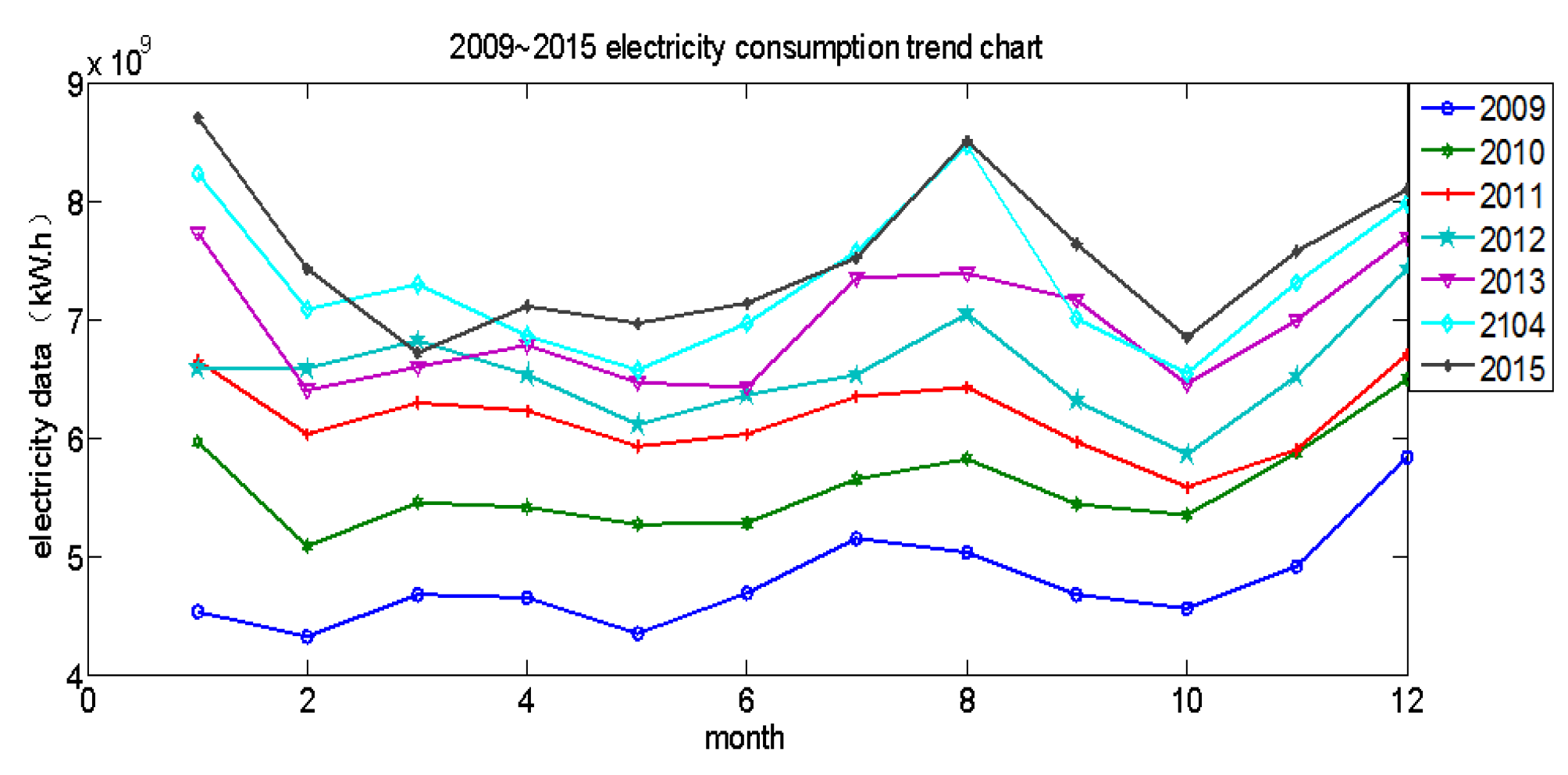
In this work, we mainly focus on predicting the EC of Shaanxi Province, China by using the proposed model. We have collected the EC data each month from 2009 to 2015 in Shaanxi Province. The trend of the EC is given in Figure 1. One can observe that although the EC fluctuated among the different years, the trend of the EC for every year was essentially identical. This primary result indicates that the EC has a certain regularity, and it is predictable.
The main factors affecting EC are the economy, climate, electricity structure, electricity and so on. After analyzing the existing data, from the point of view that it can best reflect the change in EC, this paper chooses historical EC data, gross domestic product (GDP), and the regional temperature for a total of three features supplemented by holidays to correct.
- (1)
- The quantity of electricity data.
According to the historical electricity data analysis above, we can roughly observe the development trend of the electricity demand. Consequently, it provides a profitable tool for extracting rules from that experience and knowledge to estimate the overall distribution trend in the future.
Electricity data always contains hidden information; from these historical data can be summed up the law of changes in demand for electricity; researchers on the basis of these laws can estimate the future trend of the overall distribution of the EC. In order to describe the trend of EC more clearly, this section uses the original quantity of electricity data, which is not normalized.
The historical EC is shown in Figure 1. Horizontally, there is a significant fluctuation in the amount of electricity for the 12 months of the year. First, we calculate the standard deviation of the data by the following Equation (16), and the degree of fluctuation as the proportion of the standard deviation and average value are defined. The maximum fluctuation using Equation (16) of the above data is 23.4%. Longitudinally, the amount of electricity consumed increases to different degrees every year, with an average increase of 5.21%.
where N denotes the number of the month, is the monthly electricity, and is the average annual EC.
- (2)
- Regional temperature.
For the current residential or industrial EC, there is a relationship between the temperature and the EC [27], as shown in Figure 2. In the season with a high temperature, the user’s power consumption will be greatly increased as a result of the input of refrigeration facilities such as air conditioners, and in the season with low temperature, the warmth will still consume a large amount of electric energy. Therefore, this paper also sets the temperature as an important factor affecting the EC.
- (3)
- GDP.
Economic factors, such as the development of industry and commerce, have an influence on the power system, because the rapid development of industry and commerce necessarily leads to an increase in electricity demand. In this paper, we use the GDP, which is the most representative in the field of economy, to represent economic factors.
- (4)
- Number of holidays and types of holidays.
Holidays have significant impacts on the electricity demand. In general, holiday production will be significantly reduced and electricity demand will decrease accordingly. However, the demand of electricity may increase in the Spring Festival and on the National Day because of residential electricity use substantially increasing. Accordingly, we should conduct an analysis of the characteristics of the local electricity demand to confirm the change in its trend (i.e., increasing or decreasing). Finally, after predicting the user’s EC using the proposed scheme, the prediction result may also be corrected according to the holidays.
3.3. Parameter Optimization
When the LSSVM model is used find to the quantity of electricity, the kernel parameters and the regularization parameter have a very important effect for the prediction accuracy; thus they need to be optimized firstly. The grid optimization method and K-fold cross-validation are combined to optimize the parameters in this paper. The reasons and principle introduction are as follows:
Using this combination algorithm is simple and direct for searching the parameters of LSSVM, and the searching speed compared with the test-set parameters may be faster.
The main mechanism of the combination algorithm combination?algorithm is to divide the parameters in a predetermined range into a certain number of grids and then make the model traverse all the parameters in the grid to determine the parameters of the model performance.
Just as for the traditional LSSVM model, two parameters in the proposed ECPM need to be optimized. During the optimization process, we used the training samples to train the LSSVM model, while the MCC instead of the MSE was employed to evaluate the optimal performance obtained by the certain parameters in the set of parameters and .
In order to perform the parameter optimization, the MCC is introduced as a risk function. When the training sample does not satisfy the Gaussian distribution, it can also find the appropriate parameters, which is very helpful to improve the accuracy of the prediction of the quantity of electricity. The MCC can be expressed by Equation (17):
where is the value of the kernel width optimized by the mesh optimization method.
By Equation (17), we conclude that the larger the value of the MCC, the greater the similarity of the data between the predictive value and the real value. To this end, we select the parameters that make the MCC the maximum as the optimal parameter of the prediction model. The flow chart of the parameter optimization is shown in Figure 3.
3.4. Performance Evaluation Function (PEF)
The whole quantity forecast should also include the evaluation of the forecast results. From the rigor of the study, using a single error indicator to evaluate the results of the prediction is not reliable. As a result, we choose the mean relative error (MRE), correlation coefficient (R), and the maximum prediction error () as the error statistical index to evaluate the performance of the proposed prediction scheme, and the definitions of these are as follows:
where N stands for 12 months, is the forecasting electricity for every month, is the true electricity of every month, and is the average annual EC.
4. Prediction Results and Analysis
In this section, we have performed an experiment using Matlab2013 and the LSSVM toolkit to evaluate the prediction performance of the proposed model. Experimental data is from the national grid company of Shaanxi Province from 2009 to 2015 with a period of 1 month. The prediction accuracy of the electric quantity is influenced by many factors, including historical data, GDP growth, meteorological factors and so on.
In the forecasting of the electricity, all kinds of factors that affect the demand of electricity are analyzed. In order to find out how the factors affect the electricity demand forecasting, we obtained forecasting results by only considering electricity data first, and then obtained further prediction results that considered other factors. Two prediction datasets were used to perform the contrast analysis.
For only using the historical electricity data to make predictions, the data samples needed to be divided into prediction samples and training samples. The length of the training samples had to also be divided naturally. In the setting of the experiment, we used the data of 2009–2014 as the training sample. The training data samples were divided into four groups; in other words, we could train four times by using 6 years worth of data, as shown in Equation (21), by using the first 2 years of electricity data to predict the data of the third year, through increasing the number of training times to make up for the reduction in the data dimension.
4.1. Prediction Results of Large Industry in Shaanxi Province
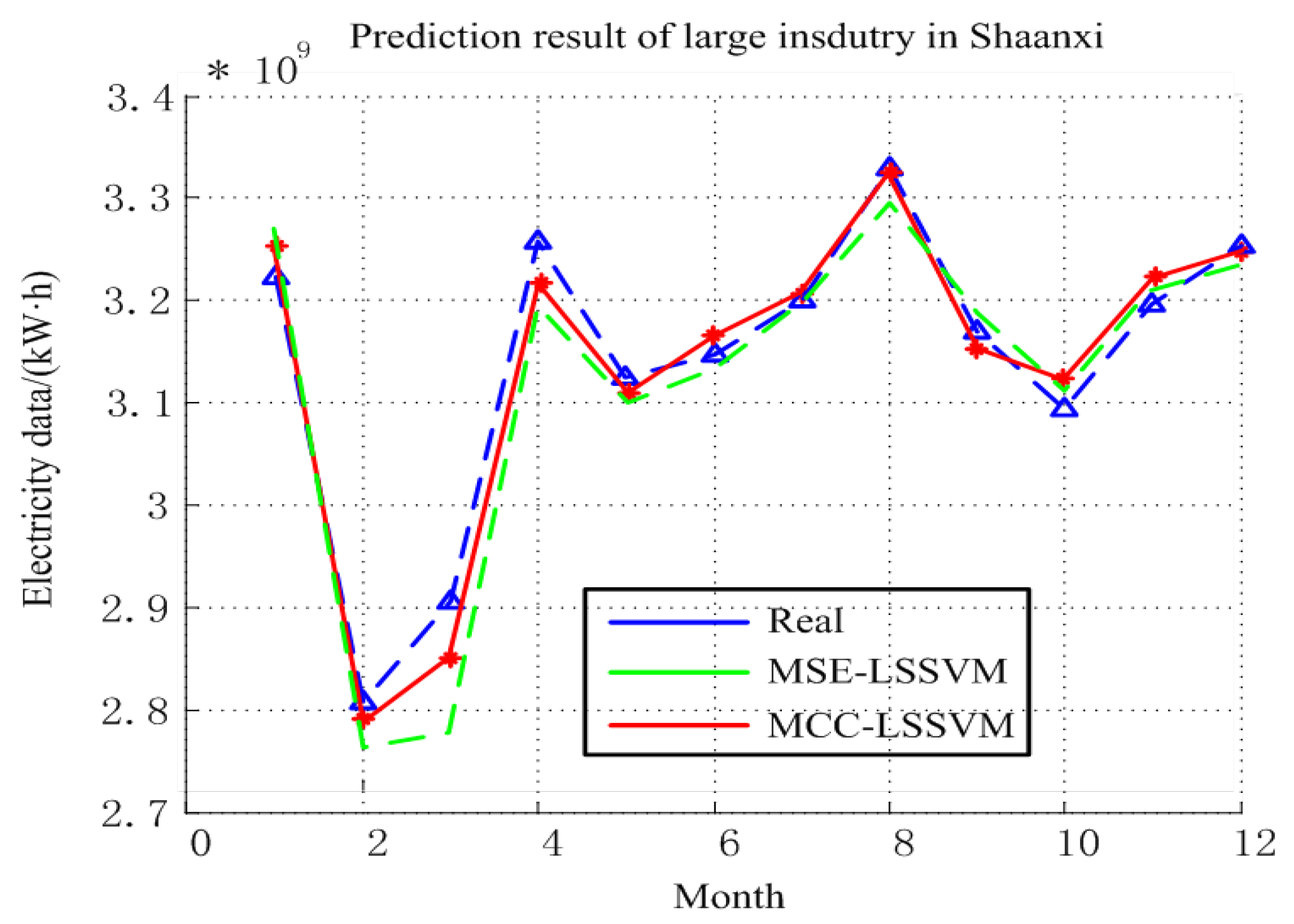
In this section, we forecast the electricity of a large industry in Shaanxi Province that is closely related to people’s lives, to research the impact of different industries on the EC using MCC–LSSVM and MSE–LSSVM. The data comes from the electricity data of the large industrial power consumption in Shaanxi Province.
The prediction results for the large industry in Shaanxi Province are shown in Figure 4, and Table 1 and Table 2. From Table 1 and Table 2, we can clearly see that the prediction error using MCC–LSSVM was 0.9% and using MSE–LSSVM was 3.12% throughout the year. We can conclude that the prediction effect of the proposed model for large industrial EC is desirable, and the reasons for this result are as follows: First, Shaanxi Province belongs to the inland city, its industrial development is relatively stable, and EC data is neat. Second, the development of the large industry and the growth of the GDP are closely related; the correlation between the two is very high, and thus the GDP factors as a result of the impact of large industrial power factors can achieve better results.
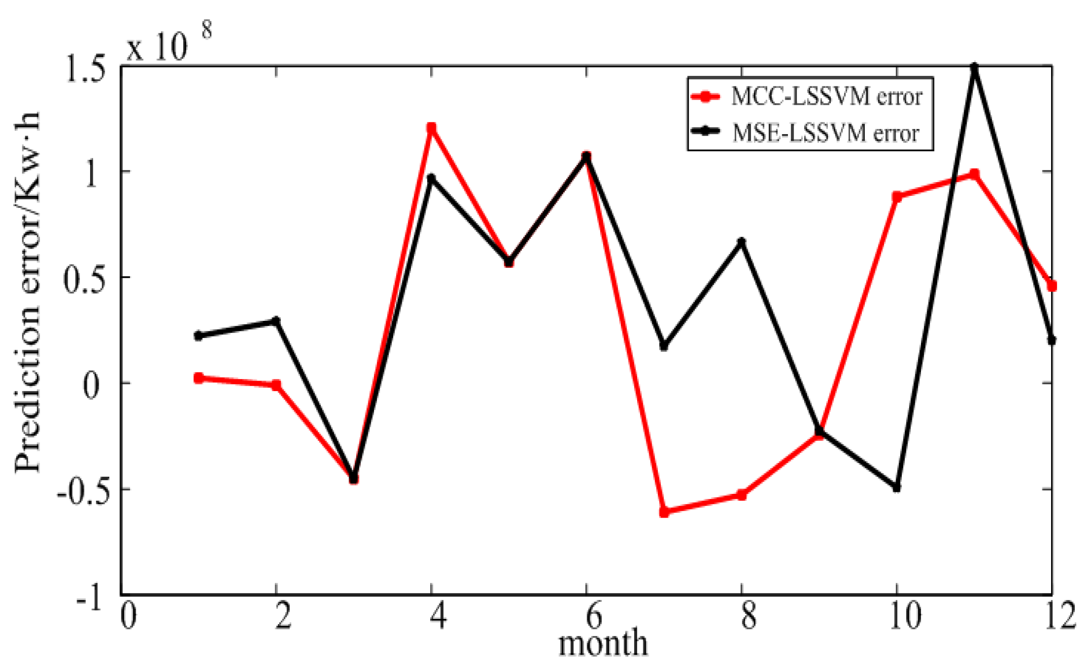
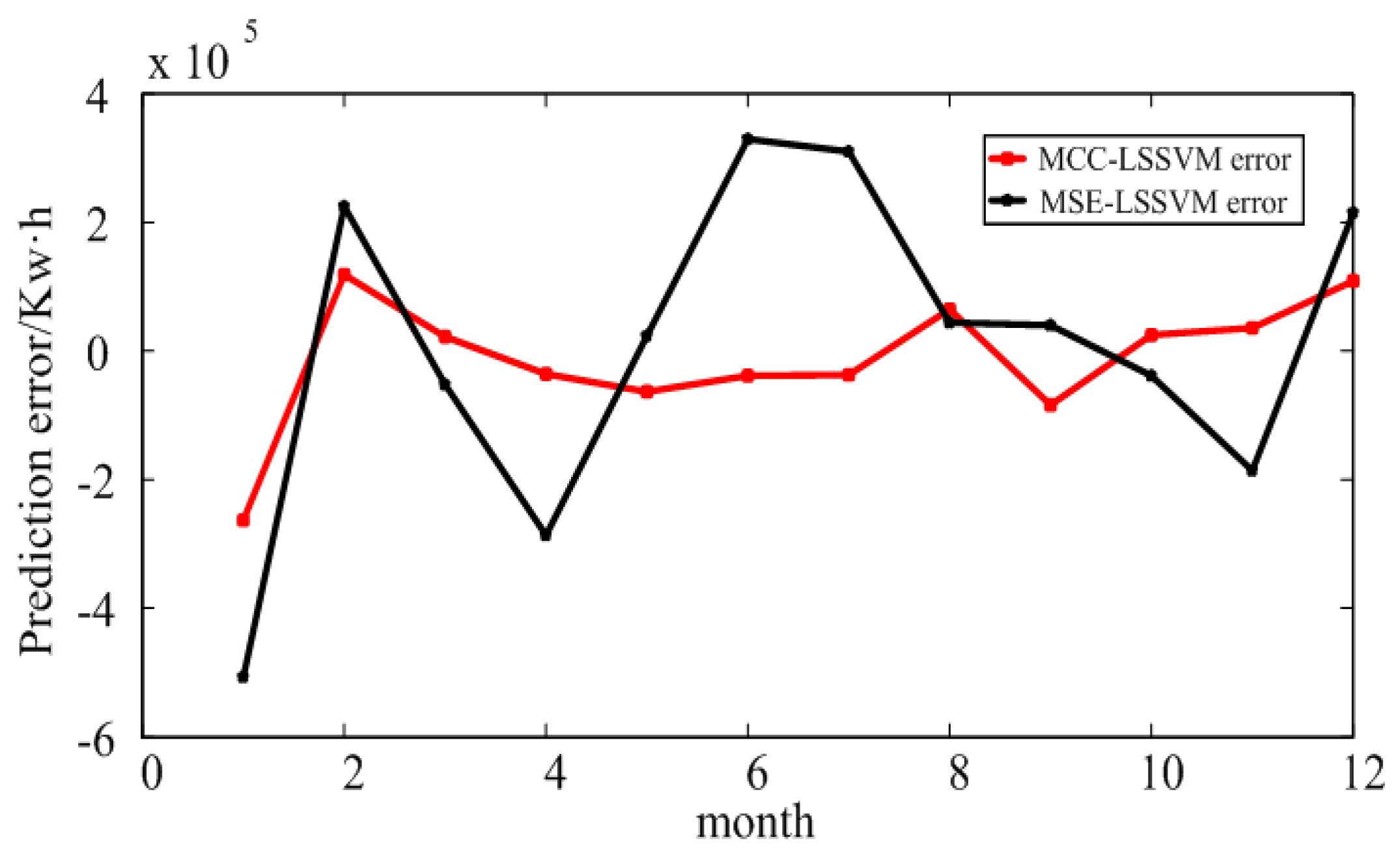
From Figure 5, one can see that the MCC–LSSVM model and MSE–LSSVM model effectively predict the regional EC. However, when using the MSE model, an error outlier appeared in March; the MCC–LSSVM model effectively suppressed the occurrence of this error outlier.
4.2. Prediction Result for Xi’an
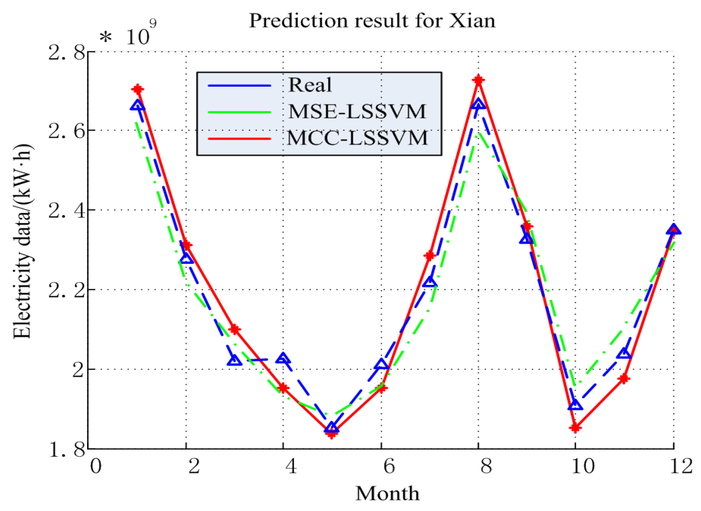
In order to verify the reliability of the proposed MCC–LSSVM model, we forecast the EC in Xi’an City, Shaanxi Province.
The MCC–LSSVM and MSE–LSSVM model prediction results and error of the power consumption in 2015 are shown in Figure 6 and Figure 7. The detailed results are given in Table 3 and Table 4. From Figure 6, one can see that the prediction result of Xi’an City was worse than for the large industry in Shaanxi Province. By Equation (18), using the MCC–LSSVM model, we obtained the annual average relative error for Xi’an of 2.77%, and the MSE–LSSVM model produced 3.23%. We explain the above results by the following two points: First, the Shaanxi Province electricity structure is more optimal, such that the power consumption data of Shaanxi Province is by contrast neater. Second, we chose the GDP as an influence factor in this experiment. As is known to all, the GDP is mainly contributed to by the manufacturing by machines; however, Xi’an is a service industry-based city. Therefore, the correlation between the GDP factor and Xi’an’s electric power development is not very strong.
4.3. Prediction Results of Electricity Consumption in an Educational Institution in Xi’an
The electricity prediction results and error in an educational institution are shown in Figure 8 and Figure 9, and Table 5 and Table 6. According to these results, one can conclude that the MCC–LSSVM model describes the change trend of the history of the electricity more accurately than the MSE–LSSVM model, and it makes an accurate prediction of the future EC. Using the above two models to predict the EC in an educational institution, we found that the prediction error of the MCC–LSSVM model was 3.98%, and the prediction error of the MSE–LSSVM model was 6.41%. At the same time, the MCC–LSSVM model effectively avoided the situation in which local errors were too large in June and July.
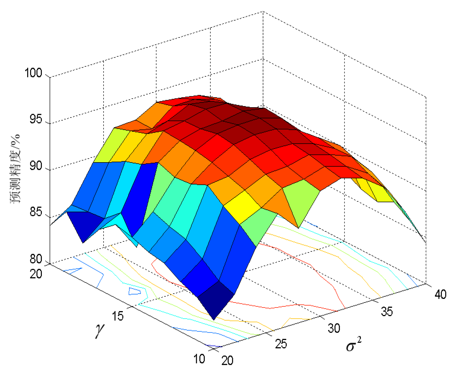
At the same time, the two key parameters of the MCC–LSSVM model are and . In the previous article, the selection of and had a great impact on the prediction accuracy. As can be seen from Figure 10, in the [10 15] interval of and for in the [20 31] interval, the increase in and increases the prediction accuracy accordingly. When and are out of the above ranges, increasing the value of these two parameters will cause varying degrees of loss in the accuracy of the prediction.
5. Conclusions
Aiming to address the current situation of the non-Gaussian characteristics in the prediction of EC, the MCC as the risk function of the LSSVM, which can effectively avoid the local error, is introduced in this paper. Furthermore, the grid optimization method and K-fold cross-validation method with shorter computational times and relatively faster search speeds are utilized to search two key parameters of the proposed model. The prediction mechanism has been evaluated for a large industry in Shaanxi Province, Xi’an City and an educational institution in Xi’an. The results show that the proposed prediction mechanism has a certain guiding value for the electricity side in formulating the electricity purchase plan and the user pricing.
Acknowledgments
This work was supported by the Nature Science Basic research program of Shaanxi Province (2014JM7255 and 2017JM6033), the Local Service Industrialization Special Plan of Shaanxi Education Department (2013JC24) and the science and technology project of China Huaneng Group (HNKJ13-H20-03).
Author Contributions
All authors wrote, reviewed and approved the manuscript. Xinyu Qiu and Wentao Ma performed the experiments. Xinyu Qiu analyzed the data.
Conflicts of Interest
The authors declare no conflict of interest.
References
- Lu, B.; Zhao, S.; Tian, Y.; Yang, Y.; Li, B.; Chen, X.; Sun, L. Mid-long term electricity consumption forecasting based on improved NGM (1,1,k) gray model. power Syst. Prot. Control 2015, 43, 98–103. [Google Scholar]
- Xue, B.; Cheng, C.; Ou, S.; Liu, A.; Wang, S. A linear regression model for forecasting monthly electricity sales considering comfortable temperature range and sudden variable. power Syst. Prot. Control 2017, 45, 15–20. [Google Scholar]
- Cao, G.; Wu, L. Support vector regression with fruit fly optimization algorithm for seasonal electricity consumption forecasting. Energy 2016, 115, 734–745. [Google Scholar] [CrossRef]
- Chae, Y.T.; Horesh, R.; Hwang, Y.; Lee, Y.M. Artificial neural network model for forecasting sub-hourly electricity usage in commercial buildings. Energy Build. 2016, 111, 184–194. [Google Scholar] [CrossRef]
- Cabral, J.D.A.; Legey, L.F.L.; de Freitas Cabral, M. Electricity consumption forecasting in Brazil: A spatial econometrics approach. Energy 2017, 126, 124–131. [Google Scholar] [CrossRef]
- Gunay, M.E. Forecasting annual gross electricity demand by artificial neural networks using predicted values of socio-economic indicators and climatic conditions: Case of Turkey. Energy Policy 2016, 90, 92–101. [Google Scholar] [CrossRef]
- Amber, K.P.; Aslam, M.W.; Hussain, S.K. Electricity consumption forecasting models for administration buildings of the UK higher education sector. Energy Build. 2015, 90, 127–136. [Google Scholar] [CrossRef]
- Santamouris, M.; Cartalis, C.; Synnefa, A.; Kolokotsa, D. On the impact of urban heat island and global warming on the power demand and electricity consumption of buildings—A review. Energy Build. 2015, 98, 119–124. [Google Scholar] [CrossRef]
- Zhu, X.; Han, Z. Research on LS-SVM Wind Speed Prediction Method Based on PSO. Proc. CSEE 2016, 36, 6337–6342. [Google Scholar]
- Bessa, R.J.; Miranda, V.; Gama, J. Entropy and correntropy against minimum square error in offline and online three-day ahead wind power forecasting. IEEE Trans. Power Syst. 2009, 24, 1657–1666. [Google Scholar] [CrossRef]
- Chen, B.D.; Xing, L.; Zhao, H.; Zheng, N.; Principe, J.C. Generalized Correntropy for Robust Adaptive Filtering. IEEE Trans. Signal Proc. 2016, 64, 3376–3387. [Google Scholar] [CrossRef]
- Liu, W.F.; Pokharel, P.P.; Principe, J.C. Correntropy: Properties and applications in non-Gaussian signal processing. IEEE Trans. Signal Proc. 2007, 55, 5286–5298. [Google Scholar] [CrossRef]
- Chen, B.D.; Xing, L.; Liang, J.; Zheng, N.; Principe, J.C. Steady-State Mean-Square Error Analysis for Adaptive Filtering under the Maximum Correntropy Criterion. IEEE Signal Proc. Lett. 2014, 21, 880–884. [Google Scholar]
- Chen, B.D.; Principe, J.C. Maximum correntropy estimation is a smoothed MAP estimation. IEEE Signal Proc. Lett. 2012, 19, 491–494. [Google Scholar] [CrossRef]
- Chen, B.D.; Wang, J.; Zhao, H.; Zheng, N.; Príncipe, J.C. Convergence of a Fixed-Point Algorithm under Maximum Correntropy Criterion. IEEE Signal Proc. Lett. 2015, 22, 1723–1727. [Google Scholar] [CrossRef]
- Vapnik, V.N.; Chervonenkis, A.Y. On the uniform convergence of relative frequencies of events to their probabilities. In Measures of Complexity; Springer: Cham, Switzerland, 2015; pp. 11–30. [Google Scholar]
- Chen, X.; Yang, J.; Liang, J.; Ye, Q. Recursive robust least squares support vector regression based on maximum correntropy criterion. Neurocomputing 2012, 97, 63–73. [Google Scholar] [CrossRef]
- Nie, H.; Liu, G.; Liu, X.; Wang, Y. Hybrid of ARIMA and SVMs for Short-Term Load Forecasting. Energy Procedia 2012, 16, 1455–1460. [Google Scholar] [CrossRef]
- Sidorov, D. Integral dynamical models. Singularities, signals and control. World Sci. 2014, 87, 9–12. [Google Scholar]
- Chen, B.D.; Liang, J.; Zheng, N.; Principe, J.C. Kernel least mean square with adaptive kernel size. Neurocomputing 2016, 191, 95–106. [Google Scholar] [CrossRef]
- He, R.; Zheng, W.-S.; Hu, B.-G. Maximum Correntropy Criterion for Robust Face Recognition. IEEE Trans. Pattern Anal. Mach. Intell. 2011, 33, 1561–1576. [Google Scholar] [PubMed]
- Ma, W.T.; Qua, H.; Gui, G.; Chen, B. Maximum correntropy criterion based sparse adaptive filtering algorithms for robust channel estimation under non-Gaussian environments. J. Frankl. Inst. 2015, 352, 2708–2727. [Google Scholar] [CrossRef]
- Chen, B.D.; Liu, X.; Zhao, H.; Principe, J.C. Maximum Correntropy Kalman Filter. Automatica 2017, 76, 70–77. [Google Scholar] [CrossRef]
- Izanloo, R.; Fakoorian, S.A.; Yazdi, H.S.; Simon, D. Kalman filtering based on the maximum correntropy criterion in the presence of non-Gaussian noise. Inf. Sci. Syst. 2016, 64, 500–505. [Google Scholar]
- Chen, B.D.; Xing, L.; Xu, B.; Zhao, H.; Zheng, N.; Príncipe, J.C. Kernel Risk-Sensitive Loss: Definition, Properties and Application to Robust Adaptive Filtering. IEEE Trans. Signal Proc. 2017, 65, 2888–2901. [Google Scholar] [CrossRef]
- Azadeh, A.; Ghaderi, S.F.; Sohrabkhani, S. Annual electricity consumption forecasting by neural network in high energy consuming industrial sectors. Energy Convers. Manag. 2008, 49, 2272–2278. [Google Scholar] [CrossRef]
- Zhang, Y.; Han, X.; Yang, Y.; Zhang, L.; Miao, X. A novel analysis and forecast method of electricity business expanding based on seasonal adjustment. In Proceedings of the 2016 IEEE PES Asia-Pacific Power and Energy Engineering Conference (APPEEC), Xi’an, China, 25–28 October 2016; pp. 707–711. [Google Scholar]
Figure 1.
2009–2015 electricity consumption trend chart.

Figure 2.
Scatter diagram of monthly average temperature and monthly electricity consumption.
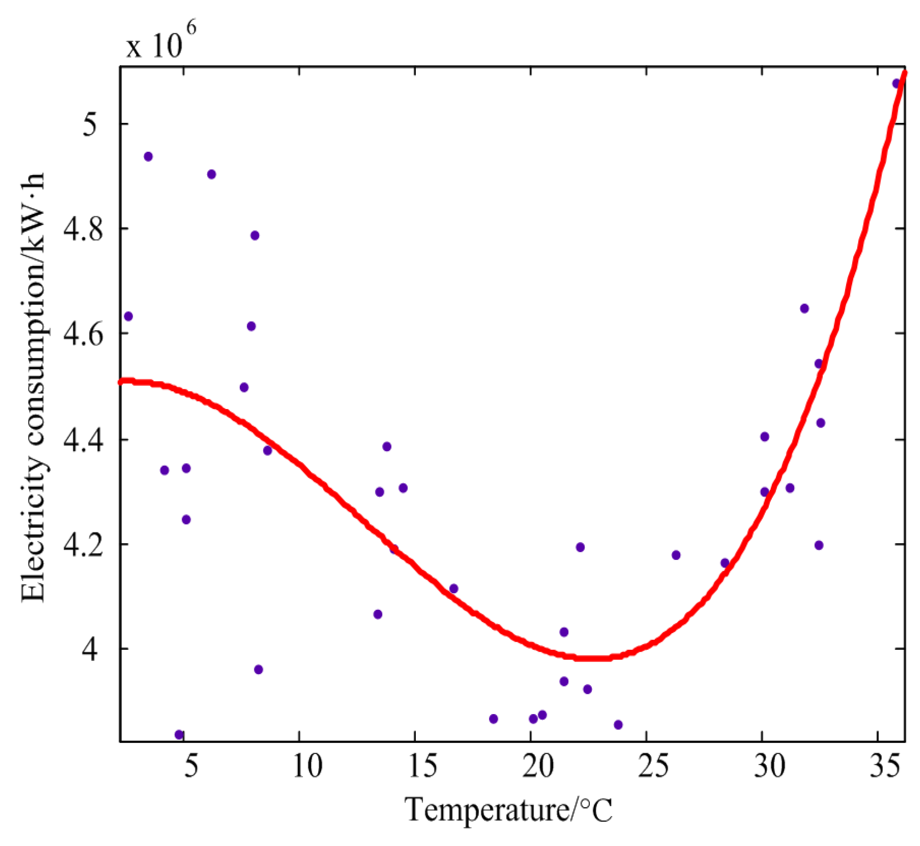
Figure 3.
Parameter optimization flow chart.
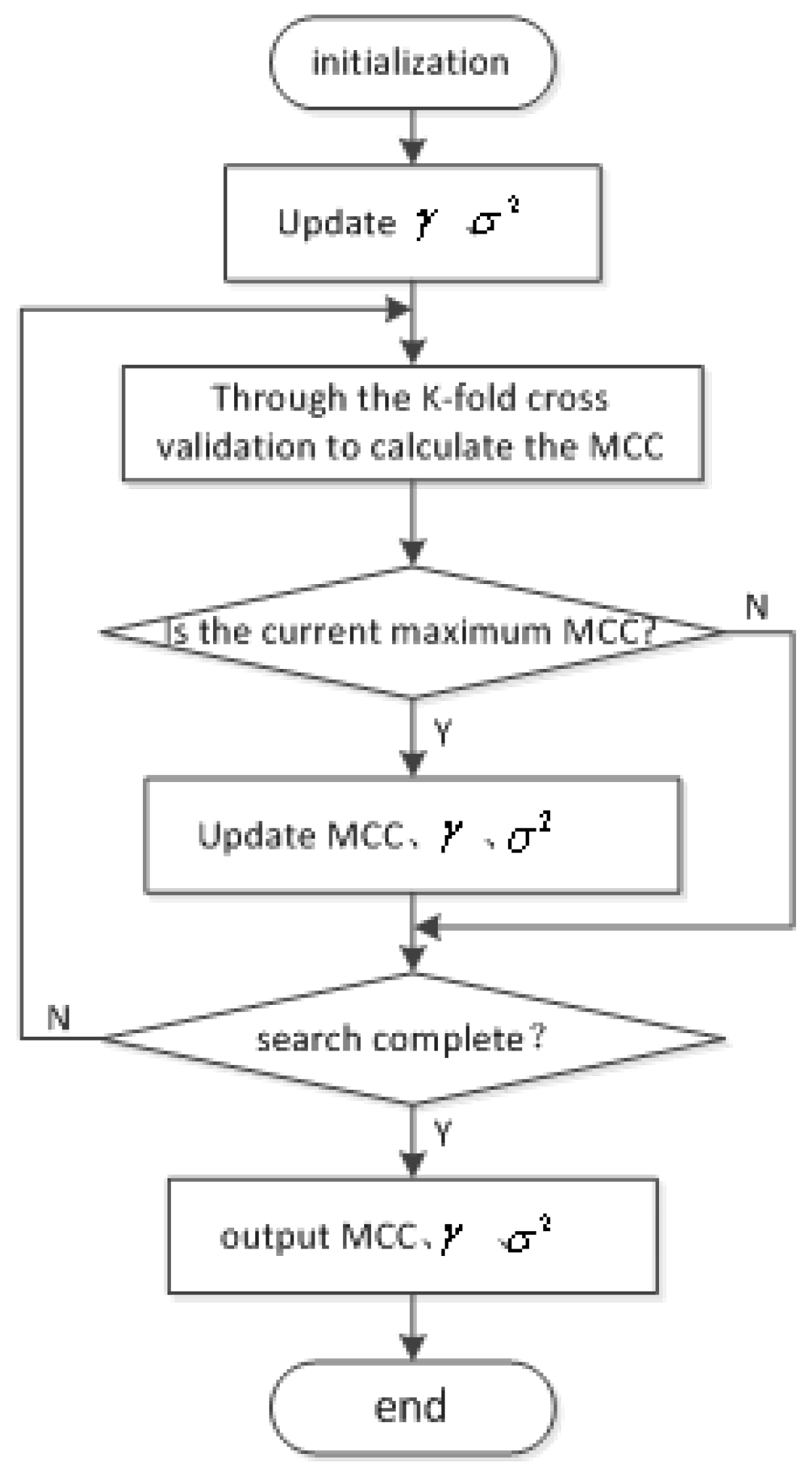
Figure 4.
Prediction results for large industry in Shaanxi Province.

Figure 5.
Prediction error for large industry in Shaanxi Province.
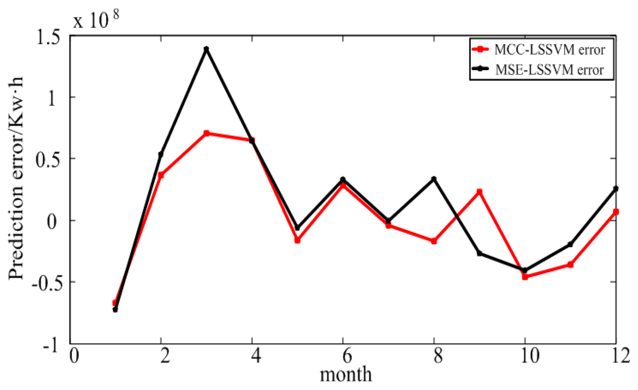
Figure 6.
Prediction result for Xi’an.

Figure 7.
Prediction error for Xi’an.

Figure 8.
Prediction results of electricity consumption in an educational institution in Xi’an.
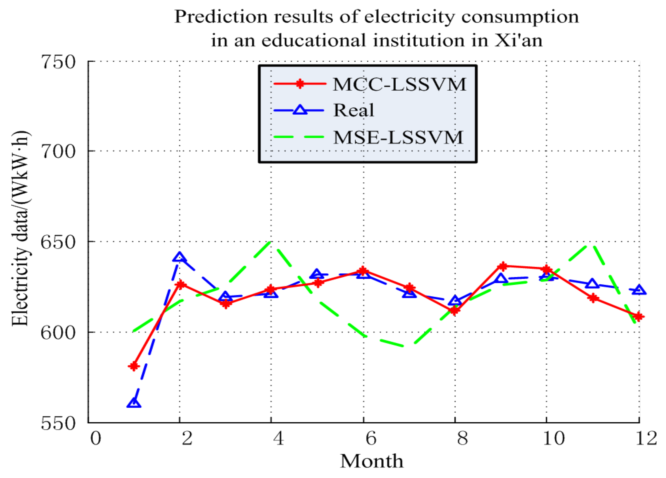
Figure 9.
Prediction error of electricity consumption in an educational institution in Xi’an.

Figure 10.
Three-dimensional map of prediction accuracy, varying with parameters and .


Table 1.
Prediction results for large industry in Shaanxi Province.
| Month | Real/kWh | MCC–LSSVM/kWh | MSE–LSSVM/kWh |
|---|---|---|---|
| 1 | 3222141989 | 3289063235 | 3294523968 |
| 2 | 2807359588 | 2770660550 | 2753838956 |
| 3 | 2905625349 | 2835276855 | 2766953282 |
| 4 | 3258028408 | 3193065850 | 3193625474 |
| 5 | 3123940121 | 3140143741 | 3130143486 |
| 6 | 3146763568 | 3118571548 | 3113648647 |
| 7 | 3200783187 | 3204753934 | 3201236988 |
| 8 | 3330358001 | 3347137347 | 3297138647 |
| 9 | 3169671810 | 3146624356 | 3196624769 |
| 10 | 3094490648 | 3140563342 | 3134963398 |
| 11 | 3197240745 | 3233100710 | 3216824659 |
| 12 | 3253492846 | 3246565684 | 3227682398 |
Table 2.
Evaluation index.
| Evaluation Index | MRE (%) | /kWh | R |
|---|---|---|---|
| MCC–LSSVM | 0.9 | 73256684 | 0.9235 |
| MSE–LSSVM | 3.12 | 140348494 | 0.8952 |
Table 3.
Prediction result for Xi’an.
| Month | Real/kWh | MCC–LSSVM/kWh | MSE–LSSVM/kWh |
|---|---|---|---|
| 1 | 2664166276 | 2661798254 | 2641798254 |
| 2 | 2275553927 | 2276537980 | 2246537980 |
| 3 | 2021181824 | 2066396013 | 2066396013 |
| 4 | 2025719576 | 1904917602 | 1928943561 |
| 5 | 1850231091 | 1792863625 | 1792863625 |
| 6 | 2011974726 | 1904917602 | 1872354896 |
| 7 | 2215976398 | 2276963182 | 2192662853 |
| 8 | 2664937423 | 2717665734 | 2596348624 |
| 9 | 2326022304 | 2350413608 | 2348629858 |
| 10 | 1906840712 | 1818905227 | 1956189345 |
| 11 | 2038734324 | 1940165576 | 1889654236 |
| 12 | 2350000000 | 2303946621 | 2329946654 |
Table 4.
Evaluation index.
| Evaluation Index | MRE (%) | /kWh | R |
|---|---|---|---|
| MCC–LSSVM | 2.77 | 120801974 | 0.9534 |
| MSE–LSSVM | 3.23 | 145653478 | 0.9316 |
Table 5.
Prediction results of electricity consumption in an educational institution in Xi’an.
| Month | Real/kWh | MCC–LSSVM/kWh | MSE–LSSVM/kWh |
|---|---|---|---|
| 1 | 5526468 | 5789523 | 6034028 |
| 2 | 6435286 | 6317452 | 6211205 |
| 3 | 6215832 | 6194268 | 6268253 |
| 4 | 6231532 | 6267145 | 6518210 |
| 5 | 6231102 | 6294423 | 6207253 |
| 6 | 6315468 | 6354652 | 5986242 |
| 7 | 6221536 | 6258553 | 5912131 |
| 8 | 6189358 | 6124125 | 6145128 |
| 9 | 6294825 | 6378632 | 6255368 |
| 10 | 6314653 | 6290058 | 6353895 |
| 11 | 6277436 | 6219389 | 6503896 |
| 12 | 6231862 | 6123568 | 6017658 |
Table 6.
Evaluation index.
| Evaluation Index | MRE (%) | /kWh | R |
|---|---|---|---|
| MCC–LSSVM | 3.98 | 2635648 | 0.9619 |
| MSE–LSSVM | 6.41 | 3296821 | 0.9106 |
© 2018 by the authors. Licensee MDPI, Basel, Switzerland. This article is an open access article distributed under the terms and conditions of the Creative Commons Attribution (CC BY) license (http://creativecommons.org/licenses/by/4.0/).
Share and Cite
MDPI and ACS Style
Duan, J.; Qiu, X.; Ma, W.; Tian, X.; Shang, D. Electricity Consumption Forecasting Scheme via Improved LSSVM with Maximum Correntropy Criterion. Entropy 2018, 20, 112. https://doi.org/10.3390/e20020112
AMA Style
Duan J, Qiu X, Ma W, Tian X, Shang D. Electricity Consumption Forecasting Scheme via Improved LSSVM with Maximum Correntropy Criterion. Entropy. 2018; 20(2):112. https://doi.org/10.3390/e20020112
Chicago/Turabian StyleDuan, Jiandong, Xinyu Qiu, Wentao Ma, Xuan Tian, and Di Shang. 2018. "Electricity Consumption Forecasting Scheme via Improved LSSVM with Maximum Correntropy Criterion" Entropy 20, no. 2: 112. https://doi.org/10.3390/e20020112
Note that from the first issue of 2016, this journal uses article numbers instead of page numbers. See further details here.