Sparse Trajectory Prediction Based on Multiple Entropy Measures

Abstract

Trajectory prediction is an important problem that has a large number of applications. A common approach to trajectory prediction is based on historical trajectories. However, existing techniques suffer from the “data sparsity problem”. The available historical trajectories are far from enough to cover all possible query trajectories. We propose the sparsity trajectory prediction algorithm based on multiple entropy measures (STP-ME) to address the data sparsity problem. Firstly, the moving region is iteratively divided into a two-dimensional plane grid graph, and each trajectory is represented as a grid sequence with temporal information. Secondly, trajectory entropy is used to evaluate trajectory’s regularity, the L-Z entropy estimator is implemented to calculate trajectory entropy, and a new trajectory space is generated through trajectory synthesis. We define location entropy and time entropy to measure the popularity of locations and timeslots respectively. Finally, a second-order Markov model that contains a temporal dimension is adopted to perform sparse trajectory prediction. The experiments show that when trip completed percentage increases towards 90%, the coverage of the baseline algorithm decreases to almost 25%, while the STP-ME algorithm successfully copes with it as expected with only an unnoticeable drop in coverage, and can constantly answer almost 100% of query trajectories. It is found that the STP-ME algorithm improves the prediction accuracy generally by as much as 8%, 3%, and 4%, compared to the baseline algorithm, the second-order Markov model (2-MM), and sub-trajectory synthesis (SubSyn) algorithm, respectively. At the same time, the prediction time of STP-ME algorithm is negligible (10 $\mathsf{\mu }\mathrm{s}$), greatly outperforming the baseline algorithm (100 $\mathrm{ms}$).

1. Introduction

As the usage of Global Positioning System (GPS) and smart mobile devices (SMD) becomes a part of our daily lives, we benefit increasingly from various types of location-based services (LBSs), such as route finding and location-based social networking. A number of new location-based applications require trajectory prediction, for example, to recommend sightseeing places, and to send targeted advertisements based on destination. Trajectory prediction has become one of the focuses for research and applications within the area of LBSs. Numerous studies have demonstrated that there is a high potential predictability in people mobility [1,2]. Lian et al. [3] put forward a collaborative exploration and periodically returning model (CEPR) exploiting a novel problem, exploration prediction (EP), which forecasts whether people will seek unvisited locations to visit. Yao et al. [4] proposed an algorithm to predict human mobility in tensors of high-dimensional location context data. Using the tensor decomposition method, Yao et al. extracted human mobility patterns with multiple expressions and then synthesized the future mobility events based on mobility patterns. Alahi et al. [5] proposed a long short-term memory (LSTM) model which can learn general human movement and predict their future trajectories. Qiao et al. [6] proposed a three-in-one Trajectory-Prediction (TP) model in road-constrained transportation networks called TraPlan. TraPlan contains three essential techniques: (1) constrained network R-tree (CNR-tree), which is a two-tiered dynamic index structure of moving objects based on transportation networks; (2) a region-of-interest (RoI) discovery algorithm, which is employed to partition a large number of trajectory points into distinct clusters; and (3) a Trajectory-Prediction (TP) approach based on frequent trajectory patterns (FTP) tree, called FTP-mining, which is proposed to discover FTPs to infer future locations of objects within RoIs. The Markov chain (MC) model has been adopted by a number of works on predicting human mobility [7,8] to incorporate some amount of memory. Second-order MC has the best accuracies, up to 95%, for predicting human mobility, and higher order MC (>2) is not necessarily more accurate, but is often less precise. Abdel-Fatao et al. [9] demonstrated that the temporal information of a trajectory provides more accurate results for predicting the destination of the trajectory. However, the above methods suffer from the “data sparsity problem”, so that many irregular patterns are contained in the huge trajectory space or only a small portion of query trajectories can match completely with the existing trajectories.

To address the data sparsity problem of trajectory prediction, Xue et al. [10,11] proposed a novel method based on the sub-trajectory synthesis (SubSyn) algorithm. The SubSyn algorithm first decomposes historical trajectories into sub-trajectories comprising two adjacent locations and builds the first-order Markov transition model, then connects the sub-trajectories into “synthesized” trajectories for destination prediction. However, the above method has some drawbacks: (1) the trajectory space is so large that the time taken by sub-trajectory synthesis is very long; (2) the prediction accuracy may be reduced because of some abnormal trajectories which influence the reliability of “synthesized” trajectories in the trajectory space; and (3) the temporal dimension and popularity of locations are ignored. For the above drawbacks, this paper proposes a sparse trajectory prediction method based on entropy estimation and a second-order Markov model. Firstly, we conduct a spatial iterative grid partition for the moving region of trajectories, and then the trajectory can be represented as a sequence of grid cells with temporal information. Secondly, we use an L-Z entropy estimator [12,13] to evaluate trajectory regularity [2] and implement it to compute the L-Z entropy of a trajectory sequences. Thirdly, we conduct trajectory synthesis based on the trajectory L-Z entropy and put synthesized trajectories into a new trajectory space. The trajectory synthesis can not only resolve the sparse problem of trajectory data, but also make the new trajectory space smaller and more credible. Fourthly, we define location entropy and time entropy to measure the popularity of locations and times, respectively. Finally, we combine location entropy and time entropy with the second-order Markov model for destination prediction under the new trajectory space.

The remainder of this paper is organized as follows: in Section 2, we introduce the spatial iterative grid partition and representations of trajectory sequences with time; in Section 3, the trajectory synthesis based on the L-Z entropy estimator is introduced; in Section 4, we define the location entropy and time entropy, and also provide an introduction of a sparsity trajectory prediction algorithm based on entropy estimation and the second-order Markov model; in Section 5, we show the experiments and results to demonstrate the effectiveness of the algorithm; and in Section 6 is the conclusion.

2. Trajectory Sequence with Time Based on Spatial Iterative Grid Partition

A common approach to a moving region spatial partition is uniform grid partitioning with a fixed size. Actually, when people browse maps on the Internet, the view of the map is different from different scales. The same size of the map includes different amounts of geographical elements from different scales, which is caused by map accuracy. The fewer geographical elements that the same sized rectangular region of map includes, the higher the geographical precision of the geographical elements represented by the map. Similarly, for the same size sample space, the more meticulous sample space partition would make the trajectory sequence much closer to the original trajectory. It is easy to divide the related GPS points into different grids by a uniform grid partition with the same size. It may separate GPS point classes into error grids. Figure 1 shows that the four GPS points are very close on the spatial location. However, they are divided into different grids because of the uniform grid partition. Thus, the connection between them is separated and it may affect the results of trajectory mining greatly.

2.1. Spatial Iterative Grid Partition

We proposed a spatial iterative grid partition (SIGP) to solve the above problem. As illustrated in Figure 2, moving regions with dense GPS point coverage will be partitioned into more grids with each grid having iteratively smaller areas by SIGP. This improves the precision of the grid to double with each iterative grid partition. Due to the continual spatial iterative grid partition for moving regions with dense GPS point coverage, the size of each grid cell will reach a suitable value and all grids include even geographical elements.

Uniform partition divides the space into a two-dimensional grid through only one partition. A trajectory can be represented as a sequence of cells according to the sequence of GPS points in the trajectory. In SIGP, the space is partitioned in multiple times. We repeat the partition process recursively until a desired grid granularity is reached. SIGP yields a more balanced number of points in each cell than a uniform grid. This leads to better prediction accuracy.

The spatial iterative grid partition algorithm is shown as follows:

Algorithm 1. Spatial Iterative Grid Partition (SIGP)
Input: D(GPS points dataset of historical trajectory), d (initial partition parameter), n(GPS point threshold of each grid)
Output: G (iterative partition grid set)
1.	Partition the moving region to $d\times d$ grid cells with the same size $\{g_{0,i}|0\le i\le (d\times d)\}$ // Divide the initial space of moving object into $d\times d$ grid cells
2.	for each grid $g_{0,i}$ in $\{g_{0,i}|0\le i\le (d\times d)\}$
3.	num = $count(g_{0,i})$         // Count the points located in each grid cell
4.	if num $\ge$ n then          // These grid cells need further dividing
5.	Excecute $Iterate-Partion(G,g_{0,i},n)$  // Call the iteration algorithm
6.	else
7.	G.push($g_{0,i}$)           //Put into the result set G
8.	end
9.	end

In Algorithm 1, each dimension of the moving region is divided into d fragments so that the moving region is divided into $d\times d$ same size grid cells. The width and height of each grid cell is $W_{0i}$ and $H_{0i}$. Parameter n is the partitioning condition for every grid cell. If the grid contains more than n GPS points, it should be divided into four grid cells again. Otherwise, the grid cell is considered as “local sparsity”. The parameter n reflects the locality of moving region partitioned by the SIGP algorithm. For the grid cell containing more than n GPS points, we use the Algorithm 2 Iterate-Partition to partition the grid cell. The process of the Algorithm Iterate-Partition is recursive to reflect the hierarchical partition characteristic of SIGP algorithm.

Algorithm 2. Iterate-Partition
Input: $G$ (iterative partition grid set), $g_i$ (grid need to be divided)； n(GPS point threshold of each grid)
Output: $G$ (iterative partition grid set)
1.	Divide $g_i$ into  four  grid cells $\{g_{i+1,j}|0\le j\le 3,H_{i+1,j}=H_{i,j}/2,W_{i+1,j}=W_{i,j}/2\}$
2.	Count the points in $g_{i+1,j}$ as $count(g_{i+1,j})$
3.	if $count(g_{i+1,j})\ge n$ then
4.	$Iterate-Partion(G,g_{i+1,j},n)$
5.	else
6.	add $g_{i+1,j}$ into $G$
7.	return $G$
8.	end

2.2. Trajectory Description Based on SIGP and Time

Nowadays, trajectory data are collected as GPS points with timestamps. These original GPS points cannot be used for trajectory prediction and they require serialization.

Firstly, we decompose each day into non-overlapping timeslots $T=\{t_1,t_2,t_3,\cdots ,t_N\}$.

Each original trajectory can be presented by a sequence of n points, each with a timestamp. Formally:

$$tra={\{(t_k,lo{n}_k,la{t}_k)|t_k<t_{k+1}\}}_{k=1}^N$$

(1)

where $t_k$, $lo{n}_k$, $la{t}_k$ denote the $kth$ GPS point’s time, longitude, and latitude.

The map is constructed as a two-dimensional grid graph which consists of $G$ by SIGP. All coordinate points are chronologically mapped to the grid graph so that a trajectory can be represented as a sequence of grid cells according to the sequence of locations of the trajectory. Formally:

$$tra={\{(t_k,g_k)|t_k\in T\}}_{k=1}^N$$

(2)

where $g_k$ is the grid in the grid graph of trajectory sequence at timeslot $t_k$.

For the same timeslots $t_i=t_j$, if consecutive grids $g_i=g_j$, $g_i$, and $g_j$ are combined into one grid cell. Similarly, we combine all the neighboring and same grid cells of trajectory sequence:

$$tra={\{(t_k,g_k)|t_k\ne t_{k+1},g_k\ne g_{k+1}\}}_{k=1}^M,M<N$$

(3)

3. Trajectory Synthesis Based on L-Z Entropy Estimation

The main idea of trajectory synthesis based on L-Z entropy estimation is an L-Z entropy estimator, which is used to evaluate trajectory’s regularity and calculate the entropy value of trajectory sequence. A new trajectory space with stronger regularity is generated by doing trajectory synthesis based on L-Z entropy.

3.1. Trajectory Entropy

Entropy can be used to quantify uncertainty, complexity, randomness, and regularity [14]. In recent decades, entropy has come to be applied very broadly [15]. We use trajectory entropy to evaluate the trajectory’s regularity. We implement the L-Z entropy estimation on the basis of Lempel–Ziv complexity [12] and use it to compute the entropy of trajectory sequence.

Trajectories are treated as time series data and trajectory entropy is introduced as a measure of regularity of sequential data in time series analysis. For a trajectory sequence $tra={\{(t_k,g_k)\}}_{k=1}^M$, the L-Z entropy can be computed by Equation (4):

$$E(tra)={(\frac{1}{M}{\displaystyle \sum _{k=2}^M\frac{{\mathsf{\Lambda }}_k}{{\log }_2(k)}})}^{-1}$$

(4)

where $M$ is the number of grid cells of trajectory $tra$; ${\mathsf{\Lambda }}_k$ is defined as the length of the shortest sub-trajectory starting at position $k$ that did not occur in the trajectory ${\{(t_k,g_k)\}}_{k=1}^M$ previously. It has been proven that $E(tra)$ converges to the actual entropy when $m$ approaches infinity [2,16]. The smaller the entropy is, the stronger the trajectory’s regularity is, and vice versa.

3.2. Trajectory Synthesis Based on Entropy Estimation

It is obvious that there are some abnormal trajectories which affect prediction accuracy in the trajectory space. To enhance the regularity of the trajectory space, we do trajectory synthesis based on trajectory entropy and put synthesized trajectories into the trajectory space. Firstly, the map is constructed as a finer grid to create less overlap between the trajectories. For each trajectory $tr{a}_i$, the entropy $e_i$ of $tr{a}_i$ is computed. Thus, the trajectory space can be obtained and the trajectories are sorted by entropy value ${\{(tr{a}_i,e_i)|e_i\le e_{i+1}\}}_{i=1}^n$. Then m (the trajectory selection parameter we can set) trajectories, which have comparatively low entropy values, are chosen (higher regularity) as the new trajectory space. For every trajectory of the new trajectory space, if there are cross-nodes with other trajectories, divide them into sub-trajectories by these cross-nodes. Then we compute the sub-trajectories’ entropy by L-Z entropy estimation. The sub-trajectories are sorted by the sequence of nodes of the trajectory that is going to be synthesized. We keep the sub-trajectories that have lower entropy if there is overlapping among them (those sub-trajectories of the trajectory that is going to be synthesized). Finally, the remainder sub-trajectories with lower entropy are synthesized. The trajectory synthesis algorithm is shown as Algorithm 3.

Algorithm 3. Trajectory Synthesis Algorithm Based on Entropy Estimation (TS-EE)
Input: $Tra={\left\{tr{a}_i\right\}}_{i=1}^n$ (historical trajectory space), m(trajectory selection parameter)
Output: $SynTra$ (synthesized trajectory space)
1.	$Sub\_Tra=\varnothing$               //Store sub_trajectories
2.	foreach $tr{a}_i$ in $Tra$
3.	$e_i=E(tr{a}_i)$ as $(tr{a}_i,e_i)$
4.	$Tra={\{(tr{a}_i,e_i)|e_i\le e_{i+1}\}}_{i=1}^n$     // Arrange $Tra={\{(tr{a}_i,e_i)\}}_{i=1}^n$ by entropy
5.	$SynTra={\{(tr{a}_i,e_i)|e_i\le e_{i+1}\}}_{i=1}^m$ // Choose the minimum entropy of $m$ trajectories in $Tra$
6.	foreach $tr{a}_i$ in $SynTra$
7.	foreach $tr{a}_k\ne tr{a}_i$ in $SynTra$
8.	$cross\_nodes(tr{a}_k,tr{a}_i)$     // Find all cross_nodes between $tr{a}_i$ and $tr{a}_k$
9.	$Sub\_Tra=divide(tr{a}_k,tr{a}_i)$ // Divide $tr{a}_i$ and $tr{a}_k$ into sub_trajectories by cross_nodes
10.	foreach $sub\_tr{a}_i$ in $Sub\_Tra$
11.	$E(sub\_tr{a}_i)$            // Compute entropy of $sub\_tr{a}_i$
12.	if $overlap(sub\_tr{a}_i,tr{a}_i)$ // $sub\_tr{a}_i$ corresponds to sub_trajectories of $tr{a}_i$ has overlap
13.	min{$E(sub\_tr{a}_i)$}     // Keep sub_tra with minimum entropy
14.	$remove(sub\_tr{a}_j|E(sub\_tr{a}_j)>E_{\min }(sub\_tr{a}_i))$  // Remove others from $Sub\_Tra$
15.	$syn\_tr{a}_i=$ $replace(tr{a}_i,sub\_tr{a}_i)$ // Replace sub_tras of $tr{a}_i$ with sub_tras in $Sub\_Tra$
16.	$add(syn\_tr{a}_i)$               // Add $syn\_tr{a}_i$ into $SynTra$
17.	return $SynTra$

4. Sparse Trajectory Prediction Based on Multiple Entropy Measures

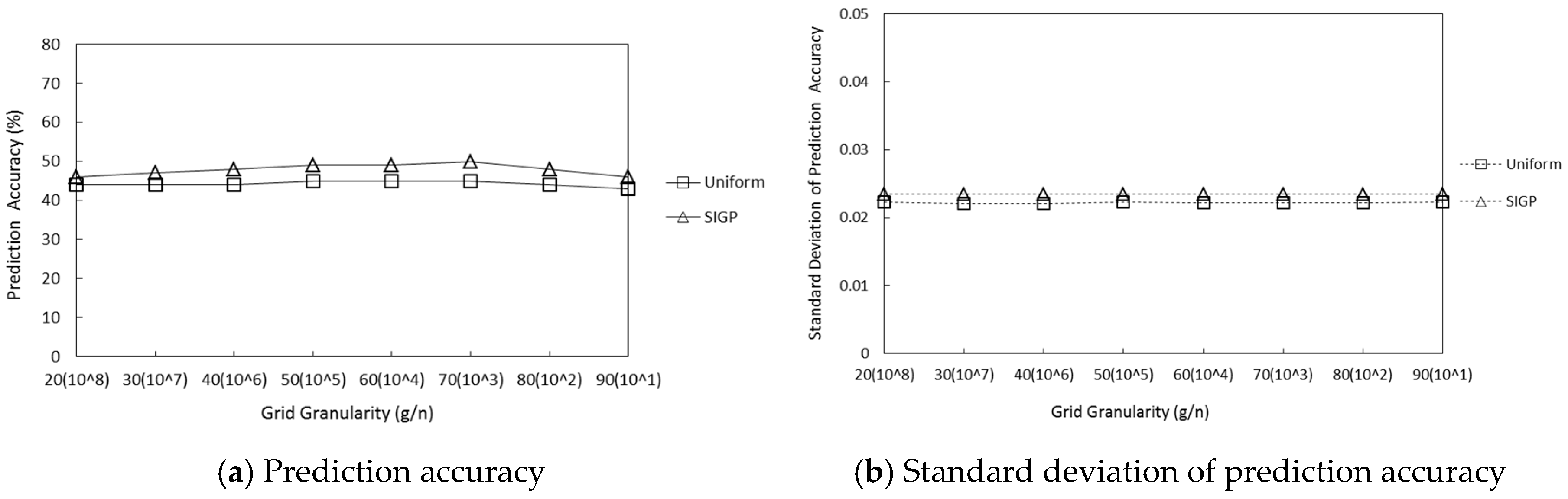
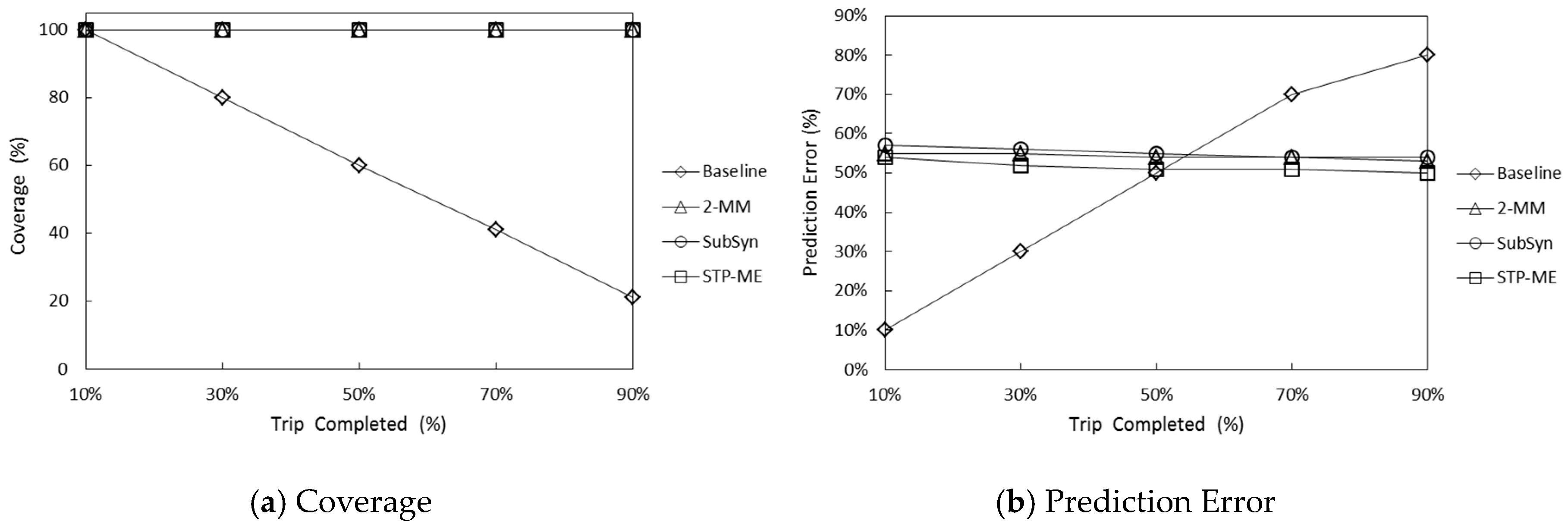
Under the smaller and more credible trajectory space generated by TS-EE, sparse trajectory prediction based on multiple entropy measures (STP-ME) combines Location entropy and time entropy with the second-order Markov model to do sparse trajectory prediction.

4.1. Location Entropy

The location entropy measures how popular a location is in terms of the people who visited it. In information theory, it is the amount of information about the users’ trajectories that visited location l. The first obvious observation is that the more visitors at l, the lower the entropy and the higher the prediction. However, the popularity of a location cannot always be described by just using the number of the visitors at the location, and this is where the entropy comes into play.

Location entropy measures the diversity of unique visitors of a location. A low value of the location entropy indicates a popular place with many visitors. Formally, the location entropy of location can be computed as:

$$E(l)=-{\displaystyle \sum _{u,V_{l,u}\ne 0}\frac{V_{l,u}}{V_l}\ln \frac{V_{l,u}}{V_l}}$$

(5)

where $V_{l,u}=\left\{\left|<u,l,t>\right|\right|\forall t\}$ denotes the set of visiting location l by user u and $V_l=\left\{\left|<u,l,t>\right|\right|\forall t,\forall u\}$ is the set of visiting at location l by all users.

4.2. Time Entropy

Time entropy measures how popular a timeslot is in terms of how many locations people visited. In information theory, it is the amount of information about the locations visited at timeslot t. The first obvious observation is that the more locations at timeslot t, the lesser the entropy and the higher the prediction. However, the popularity of a timeslot cannot always be described by just using the number of the locations at the timeslot, and this is where the entropy comes into play. The advantage of using entropy is that it measures the timeslot popularity based on the number of locations over the users who visited them.

Time entropy measures the diversity of unique visitors of different time slots. Formally, the time entropy of timeslot can be computed as:

$$E(t)=-{\displaystyle \sum _{u,L_{t,u}\ne 0}\frac{L_{t,u}}{L_t}\ln \frac{L_{t,u}}{L_t}}$$

(6)

where $L_{t,u}=\left\{\left|<u,l,t>\right|\right|\forall l\}$ denotes the number of locations visited by user u at timeslot t and $L_t=\left\{\left|<u,l,t>\right|\right|\forall l,\forall u\}$ is the number of locations visited by all users at timeslot t.

4.3. Second-Order Markov Model for Trajectory Prediction

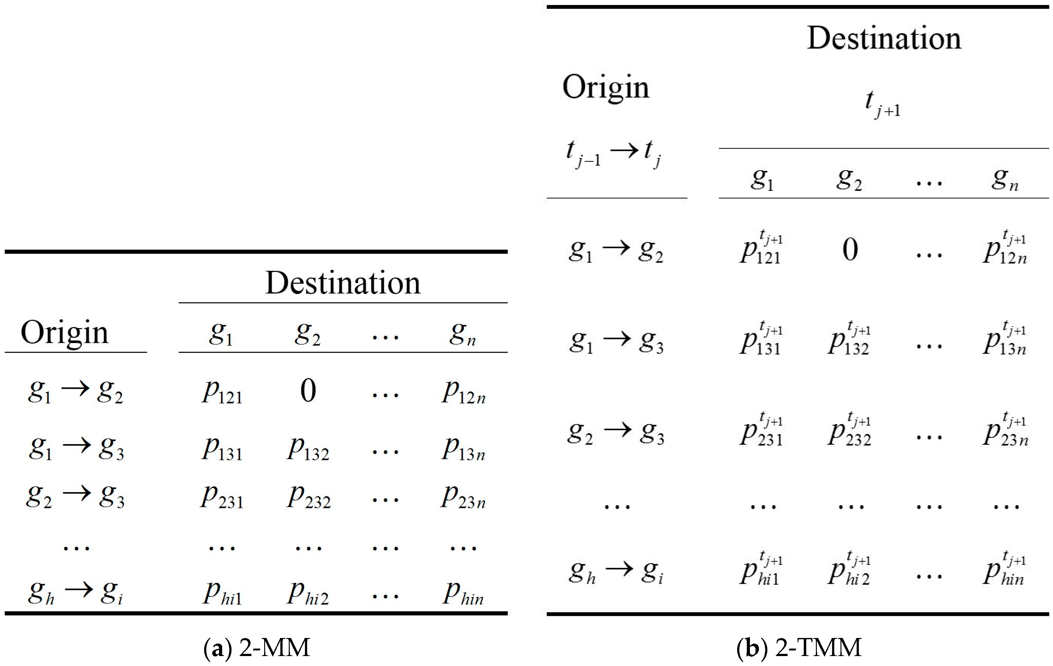
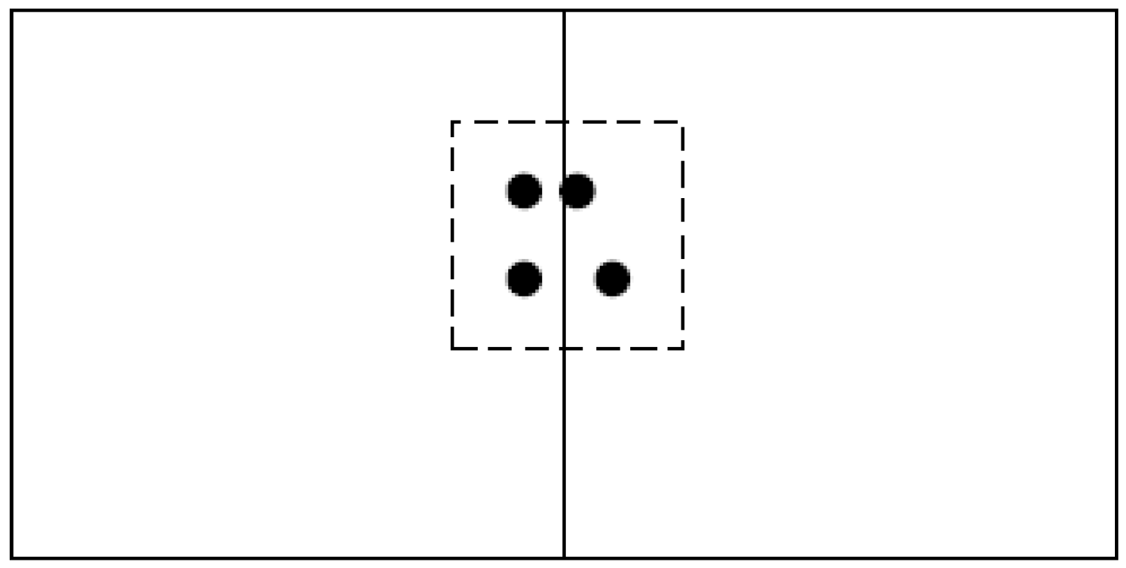
A number of studies [7,8] have established that the second-order Markov model (2-MM) has the best accuracies, up to 95%, for predicting human mobility, and that higher-order MM (>2) is not necessarily more accurate, but is often less precise. However, the 2-MM always utilizes historical geo-spatial trajectories to train a transition probability matrix and in 2-MM (see Figure 3a) the probability of each destination is computed based only on the present and immediate past grids of interest that a user visited without using temporal information. Despite being quite successful in predicting human mobility, existing works share some major drawbacks. Firstly, the majority of the existing works are time-unaware in the sense that they neglect the temporal dimension of users’ mobility (such as time of the day) in their models. Consequently, they can only tell where, but not when, a user is likely to visit a location. Neglecting the temporal dimension can have severe implications on some applications that heavily rely on temporal information for the effective function. For example, in homeland security, temporal information is vital in predicting the anticipated movement of a suspect if a potential crime is to be averted. Secondly, no existing works have focused on the popularity of locations and timeslots with considering locations users are interested in and in which timeslots users are active. Trajectory prediction accuracy would be improved by computing user’s popularity of different locations and timeslots quantitatively; for example, people are most likely to go shopping or walking in the park after work. We propose the second-order Markov model with Temporal information (2-TMM, see Figure 3b) for trajectory prediction based on location entropy and time entropy. Specifically, using Bayes rule, we find the stationary distribution of posterior probabilities of visiting locations during specified timeslots. We then build a second-order mobility transition matrix and combine location entropy and time entropy with a second-order Markov chain model for predicting most likely next location that the user will visit in the next timeslot, using the location entropy, the time entropy, the transition matrix, and the stationary posterior probability distributions.

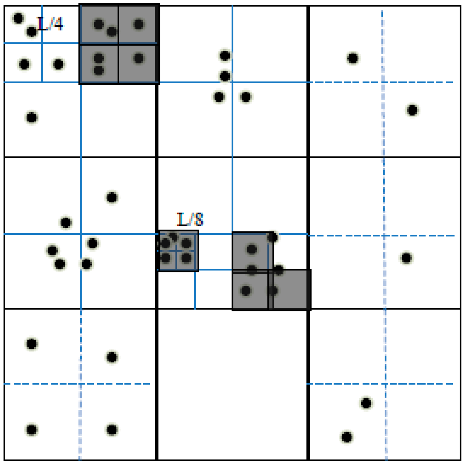
Let $G=\{g_1,g_2,g_3,\cdots ,g_n\}$ denote a finite set of grids partitioned by SIGP. Additionally, let $T=\{t_1,t_2,t_3,\cdots ,t_m\}$ be a set of predefined timeslots in a day. Thus, $tra(u)=\{(t_1,g_1),(t_2,g_2),\dots ,(t_k,g_k)\}$ denotes a finite set of historical grids with temporal information visited by user u. Assuming Table 1 represents statistics of historical visit behaviors of all users, Table 1a corresponds to trajectories’ historical visits to grids without considering temporal information, and Table 1b corresponds to trajectories’ historical visits to grids during specified timeslots, where $Frequency(g_i)={\displaystyle \sum _{t_i\in T}frequency(g_i,t_i)}$.

Definition 1. 

Given a finite set of grids with time visited by trajectories, the visit probability, denoted by $\lambda (g_i,t_j)$ of a grid $g_i\in G$, is a numerical estimate of the likelihood that users will visit grid $g_i$ during $t_j\in T$. We express a visit probability of grid $g_i$ in terms of two component probabilities coined as (i) grid feature-correlated visit probability (GVP), and (ii) temporal feature-correlated visit probability (TVP). GVP of a grid $g_i$ denoted by $P(g_i)$, is a prior probability of visit to $g_i$ expressed as a ratio of number of times trajectories visited $g_i$ to the total number of visits to all grids in the trajectories’ grid history.

Table 2a exemplifies GVP probabilities computed from Table 1a. TVP of $g_i$ during $t_j$, denoted by $P(t_j|g_i)$, is a conditional probability that a visit occurred during $t_j$ given that $g_i$ is visited by trajectories. Table 2b shows TVP probabilities obtained from Table 1b.

In line with Definition 1, we compute the visit probability of a semantic location by applying the Bayes’ rule to GVP and TVP. Accordingly, the visit probability of $g_i$ during timeslot $t_j$ is given by:

$$\lambda (g_i,t_j)=\frac{P(g_i)P(t_j|g_i)}{[P(g_i)P(t_j|g_i)]+{\displaystyle \sum _{g_n\in G,g_n\ne g_i}[P(g_n)P(t_j|g_n)]}}$$

(7)

where $0\le \lambda (g_i,t_j)\le 1$. $P(g_i)$ and $P(t_j|g_i)$ are defined in Definition 1.

Applying Equation (7) to Table 2 yields visit probabilities for grids visited during each timeslot in

Table 3. Visit probabilities.

Grid		$g_1$	$g_2$	$g_3$	…	$g_n$
$\lambda (g_i,t_j)$	$t_1$	${\lambda }_{g_1}^{t_1}$	${\lambda }_{g_2}^{t_1}$	${\lambda }_{g_3}^{t_j}$		${\lambda }_{g_n}^{t_1}$
	$t_2$	${\lambda }_{g_1}^{t_2}$	${\lambda }_{g_2}^{t_2}$	${\lambda }_{g_3}^{t_2}$		${\lambda }_{g_n}^{t_2}$
	$t_3$	${\lambda }_{g_1}^{t_3}$	${\lambda }_{g_2}^{t_3}$	${\lambda }_{g_3}^{t_3}$		${\lambda }_{g_n}^{t_3}$
					…
	$t_m$	${\lambda }_{g_1}^{t_m}$	${\lambda }_{g_2}^{t_m}$	${\lambda }_{g_3}^{t_m}$		${\lambda }_{g_n}^{t_m}$

. Each column in Table 3 is a probability vector showing a distribution of $\lambda (g_i,t_j)$ for each $g_i\in G$ during $t_j$, where ${\displaystyle \sum _{g_i\in G}\lambda (g_i,t_j)}=1$.

Definition 2. 

A second-order Markov chain model is a discrete stochastic process with limited memory in which the probability of visiting a grid $g_w$ during timeslot $t_{j+1}$ only depends on tags of two grids visited during timeslots $t_j,t_{j-1}$.

In line with Definition 2, the probability that a trajectory’s destination will be a grid $g_d$ during timeslot $t_{j+1}$ can be expressed as $P[(g_d,t_{j+1})|(g_i,t_j),(g_{i-1},t_{j-1})]$.

Definition 3. 

A transition probability $p_{hi\mathrm{d}}^j$ with respect to 2-TMM is the probability that a trajectory will move to a destination grid $g_d$ during timeslot $t_{j+1}$ given that the user has successively visited locations having tags $g_h$ and $g_i$ during timeslots $t_{j-1}$ and $t_j$, respectively.

We denote a transition from grids $g_h$ and $g_i$ during timeslots $t_{j-1}$ and $t_j$, respectively, to a destination grid $g_d$ during timeslot $t_{j+1}$ by $[g_h^{t_{j-1}},g_i^{t_j}\to g_d^{t_{j+1}}]$. The transition probability is computed as:

$$p_{hid}^j=\frac{count[g_h^{t_{j-1}},g_i^{t_j}\to g_d^{t_{j+1}}]}{{\displaystyle \sum count[g_h^{t_{j-1}},g_i^{t_j}\to g_{*}^{t_{j+1}}]{\displaystyle \sum _{g_{*}\in G}count[g_h^{t_{j-1}},g_i^{t_j}\to g_{*}^{t_{j+1}}]}}}$$

(8)

where $g_{*}$ is the tag of any location at $t_{j+1}$. We predict the destination grid $g_{pre}$ of the most likely next grid and its probability by computing right hand side of Equation (9):

$$P[(g_{pre},t_{j+1})|(g_i,t_j),(g_{i-1},t_{j-1})]=\underset{g_d\in G}{\mathrm{argmax}}\{P[(g_d,t_{j+1})|(g_i,t_j),(g_{i-1},t_{j-1})]\}$$

(9)

Let probability vectors $\lambda (t_j)$ and $\lambda (t_{j-1})$ represent distributions of visit probabilities of grids during timeslots $t_j$ and $t_{j-1}$, respectively. We represent the initial probability distribution of 2-TMM by the joint distribution of $\lambda (t_j)$ and $\lambda (t_{j-1})$ given by $\lambda (t_j{t}_{j-1})=\lambda (t_j)\lambda (t_{j-1})=\{\lambda (g_1,t_j{t}_{j-1}),\lambda (g_2,t_j{t}_{j-1}),\lambda (g_3,t_j{t}_{j-1}),\cdots ,\lambda (g_n,t_j{t}_{j-1})\}$. Given the initial probability distribution and the matrix of transition probabilities, and the location entropy and time entropy computed, the prediction destination of a target query trajectory is calculated by using:

$$P[(g_{pre},t_{j+1})|(g_i,t_j),(g_{i-1},t_{j-1})]=\underset{g_w\in G}{\mathrm{argmax}}\{{(E(g_w))}^{-1}\cdot {(E(t_{j+1}))}^{-1}\cdot {\displaystyle \sum _{g_i\in G}\lambda (g_i,t_j{t}_{j-1})\cdot }{p}_{hid}^j\}$$

(10)

5. Experimental Evaluation and Analysis of the Results

In this section, we conduct an extensive experimental study to evaluate the performance of our STP-ME algorithm. It is worth mentioning that all of the experiments were run on a commodity computer with Intel Core i5 CPU (2.3GHz) (Intel Corporation, Santa Clara, CA, USA) and 4GB RAM. We use a real-world large scale taxi trajectory dataset from the T-drive project in our experiments [17]. It contains a total of 580,000 taxi trajectories in the city of Beijing, with 15 million GPS data points from 2 February 2008 to 8 February 2008. In the follow experimental results, we select 80% trajectories in the dataset as a training dataset to infer the parameter and build the Markov model randomly, and the remainder 20% trajectories were used to estimate the coverage, prediction time, prediction error, and prediction accuracy.

5.1. The Result of Trajectory L-Z Entropy

To evaluate trajectory regularity, we divide every day into twelve periods, and then compute the average trajectory L-Z entropy for each period of time on weekend and weekday, respectively.

The results in Figure 4a clearly show that the trajectory L-Z entropies of twelve periods conform to the taxi traveling path, i.e., it is the go-to-work hours between 6:00 and 8:00, and the taxi traveling path is always regular from home to company, so the average L-Z entropy is the smallest. In Figure 4b, the standard deviation of L-Z entropy is stable. Consequently, trajectory entropy can be used to evaluate trajectory regularity.

5.2. Comparison of Various Grid Partitioning Strategies

Until now we have assumed a spatial iterative grid to represent the moving region. In this section, we investigate another grid partitioning strategy, a uniform grid partitioning. The moving region is constructed as a two-dimensional grid consisting of $g\times g$ square cells. The granularity of this representation is a cell, i.e., all the locations within a single cell are considered to be the same object. Each cell has the side length of 1 and adjacent cells have the distance of 1. The whole grid is modelled as a graph where each cell corresponds to a grid in the graph. A trajectory can be represented as a sequence of grids according to the sequence of locations of the trajectory.

The prediction accuracy of STP-ME based on spatial iterative grid partitioning and uniform grid partitioning is given in Figure 5a, where g is the grid granularity of the uniform grid partition and n is the grid partition parameter of SIGP. A suitable value of n needs to be decided for our training dataset. On one hand, a large value of n may have very low prediction accuracy because the area covered by each grid cell is too large. On the other hand, it leads to more matching query trajectories since more trajectories may fall into identical cells, hence increasing prediction accuracy. A small value of n has the advantage of higher prediction accuracy that the small cell area brings, but training data becomes even sparser because fewer locations will lie in a same cell, making the task of destination prediction more difficult. Therefore, we need to find a balanced value of n which can achieve the best prediction accuracy. The optimal grid partition parameter n for our training dataset is selected to be 10³ according to the global minimum point in Figure 5. Compared with the uniform grid, SIGP is able to achieve higher prediction accuracy with the increase of grid granularity. This is because, in a city, regions with dense trajectory coverage (e.g., Central Business District region) will be mapped to more cells with each cell having smaller areas. This improves the prediction accuracy of queries that involve these regions. The better result is given by SIGP because it achieves the most even distribution of points, which shows that SIGP has less information loss than that of the uniform grid. Figure 5b shows the standard deviation of prediction accuracy between uniform grid partition and SIGP. Standard deviation of both grid partition methods is not only small, but also stable.

5.3. The Comparison of STP-ME Algorithm with Baseline, 2-MM, and SubSyn Algorithms

To evaluate the performance of our STP-ME, we compare Prediction accuracy, prediction time, and coverage of 2-STMM with two approaches, namely, (i) the baseline algorithm coined from [7] which uses trajectory matching of historical visits; (ii) destination prediction using a second-order Markov model (2-MM) [18] to develop a second-order Markov chain model to predict the next grid that a user is likely to visit (see Figure 3a); and (iii) destination prediction by sub-trajectory synthesis (SubSyn) proposed by Xue et al. [10,11]. The prediction accuracy is computed as the ratio between the number of correctly predicted trajectories and the total number of trajectories. Prediction time is the time used to predict the destination for one query trajectory online, and the coverage counts the number of query trajectories for which some destinations are provided. We use this property to demonstrate the difference in robustness between the baseline algorithm, 2-MM, SubSyn, and our STP-ME.

Figure 6a and Figure 7a show the trend in both prediction time and prediction accuracy with respect to grid granularity. We compare the runtime performance of our STP-ME with that of the baseline algorithm, 2-MM, and SubSyn in terms of online query prediction time. Since the information is stored during the offline training stage, STP-ME requires little extra computation when answering a user’s query (10 $\mathsf{\mu }\mathrm{s}$), whereas the baseline algorithm requires too much time (100 $\mathrm{ms}$) to predict. Our STP-ME, SubSyn, and 2-MM are at least four orders of magnitudes better, constantly. The reason is that the baseline algorithm is forced to make a full sequential scan of the entire trajectory space to compute the posterior probability, whereas the other algorithms can extract most transition probability values from the visit probability distribution and a matrix of transition probabilities directly. It is worth mentioning that grid granularity has little influence on the prediction time of our STP-ME, SubSyn, and 2-MM. The predition accuracy of our STP-ME, SubSyn, and 2-MM has a slight rise with the increase of grid granularity and reaches the peak at n = 10³. The prediction accuracy of our STP-ME is about 8%, 3%, and 4% higher than that of the baseline algorithm, 2-MM, and SubSyn, respectively. For the baseline algorithm, the number of query trajectories which have sufficient destinations drops slightly as the grid granularity increases due to the fact that more trajectories in the training dataset may fall into different grids, so query trajectories are less likely to have a partial match in the trajectory space. Meanwhile, the prediction accuracy of STP-ME (48%), SubSyn (44%), and 2-MM (45%) are stable and ascend steadily. From Figure 6b, the standard deviation of prediction time on our STP-ME, SubSyn, and 2-MM is almost 0. In Figure 7b, the standard deviation of prediction accuracy obtained by our STP-ME is the smallest and stable, which means its prediction accuracy is effective and stable.

Apart from the huge advantage of STP-ME in prediction time and prediction accuracy, its coverage and prediction error are comparable with that of the baseline algorithm. Figure 8 shows the coverage and prediction error versus the percentage of the trip completed. For the baseline algorithm, the amount of query trajectories for which sufficient predicted destinations are provided decreases as the trip completed increases due to the fact that longer query trajectories (i.e., higher trip completed percentage) are less likely to have a partial match in the training dataset. Specifically, when trip completed percentage increases towards 90%, the coverage of the baseline algorithm decreases to almost 25%. Our STP-ME successfully copes with it as expected, with only an unnoticeable drop in coverage, and can constantly answer almost 100% of query trajectories. This proves that the baseline algorithm cannot handle long trajectories because the chances of finding a matching trajectory decrease when the length of a query trajectory grows. For the baseline algorithm, despite the negative influence of the coverage problem, its prediction error also increases as the trip completed percentage increases for a simple reason. When the baseline algorithm fails to find adequate predicted destinations, we use the current node in the query trajectory as the predicted destination. For STP-ME, getting closer to the true destination means that there are fewer potential destinations and, intuitively, the prediction error reduces. It is observed that STP-ME outperforms the baseline algorithm throughout the progress of a trip.

6. Conclusions

In this paper, we have proposed STP-ME to conduct sparsity trajectory prediction. STP-ME uses an L-Z entropy estimator to compute a trajectory’s L-Z entropy and provides trajectory synthesis based on a trajectory’s L-Z entropy. Lastly, by combining location entropy and time entropy, STP-ME uses a second-order Markov model to predict the destination. Experiments based on real datasets have shown that the STP-ME algorithm can predict destinations for almost all query trajectories, so it has successfully addressed the data sparsity problem. Compared with the baseline algorithm and 2-MM, STP-ME has higher prediction accuracy. At the same time, the STP-ME requires less time to predict and runs over four orders of magnitudes faster than the baseline algorithm.

References

1. Gonzalez, M.C.; Hidalgo, C.A.; Barabasi, A.L. Understanding individual human mobility patterns. Nature 2008, 453, 779–782. [Google Scholar] [CrossRef] [PubMed]
2. Song, C.; Qu, Z.; Blumm, N.; Barabási, A.-L. Limits of predictability in human mobility. Science 2010, 327, 1018–1021. [Google Scholar] [CrossRef] [PubMed]
3. Lian, D.; Xie, X.; Zheng, V.W.; Yuan, N.J.; Zhang, F.; Chen, E. CEPR: A collaborative exploration and periodically returning model for location prediction. ACM Trans. Intell. Syst. Technol. 2015, 6. [Google Scholar] [CrossRef]
4. Yao, D.; Yu, C.; Jin, H.; Ding, Q. Human mobility synthesis using matrix and tensor factorizations. Inf. Fusion 2015, 23, 25–32. [Google Scholar] [CrossRef]
5. Alahi, A.; Goel, K.; Ramanathan, V.; Robicquet, A.; Li, F.-F.; Savarese, S. Social LSTM: Human Trajectory Prediction in Crowded Spaces. Available online: http://web.stanford.edu/~alahi/downloads/CVPR16_N_LSTM.pdf (accessed on 26 August 2016).
6. Qiao, S.; Han, N.; Zhu, W.; Gutierrez, L.A. TraPlan: An Effective Three-in-One Trajectory-Prediction Model in Transportation Networks. IEEE Trans. Intell. Transp. Syst. 2015, 16, 1188–1198. [Google Scholar] [CrossRef]
7. Gambs, S.; Killijian, M.O.; Del Prado Cortez, M.N. Next place prediction using mobility Markov chains. In Proceedings of the First Workshop on Measurement, Privacy, and Mobility, Bern, Switzerland, 10–13 April 2012.
8. Smith, G.; Wieser, R.; Goulding, J.; Barrack, D. A refined limit on the predictability of human mobility. In Proceedings of the 2014 IEEE International Conference on Pervasive Computing and Communications, Budapest, Hungary, 24–28 March 2014; pp. 88–94.
9. Abdel-Fatao, H.; Li, J.; Liu, J. STMM: Semantic and Temporal-Aware Markov Chain Model for Mobility Prediction. In Data Science; Springer: Cham, Switzerland, 2015; pp. 103–111. [Google Scholar]
10. Xue, A.Y.; Zhang, R.; Zheng, Y.; Xie, X.; Huang, J.; Xu, Z. Destination prediction by sub-trajectory synthesis and privacy protection against such prediction. In Proceedings of the IEEE 29th International Conference on Data Engineering (ICDE), Brisbane, Australia, 8–12 April 2013; pp. 254–265.
11. Xue, A.Y.; Qi, J.; Xie, X.; Zhang, R.; Huang, J.; Li, Y. Solving the data sparsity problem in destination prediction. VLDB J. 2014, 24, 219–243. [Google Scholar] [CrossRef]
12. Gao, Y.; Kontoyiannis, I.; Bienenstock, E. Estimating the entropy of binary time series: Methodology, some theory and a simulation study. Entropy 2008, 10, 71–99. [Google Scholar] [CrossRef]
13. Liu, L.; Miao, S.; Cheng, M.; Gao, X. Permutation Entropy for Random Binary Sequences. Entropy 2015, 17, 8207–8216. [Google Scholar] [CrossRef]
14. Chen, B.; Wang, J.; Zhao, H.; Principe, J.C. Insights into Entropy as a Measure of Multivariate Variability. Entropy 2016, 18, 196. [Google Scholar] [CrossRef]
15. Toffoli, T. Entropy? Honest! Entropy 2016, 18, 247. [Google Scholar] [CrossRef]
16. Mclnerney, J.; Stein, S.; Rogers, A.; Jennings, N.R. Exploring Periods of Low Predictability in Daily Life Mobility. Available online: http://eprints.soton.ac.uk/339940/1/paper_extended_past2.pdf (accessed on 26 August 2016).
17. Microsoft Research: T-Drive Trajectory Data Sample. Available online: https://www.microsoft.com/en-us/research/publication/t-drive-trajectory-data-sample/ (accessed on 26 August 2016).
18. Ziebart, B.D.; Maas, A.L.; Dey, A.K.; Begnell, J.A. Navigate Like a Cabbie: Probabilistic Reasoning from Observed Context-Aware Behavior. Available online: http://www.cs.cmu.edu/~bziebart/publications/navigate-bziebart.pdf (accessed on 26 August 2016).
Figure 1. Related GPS points are divided into different grids.
Entropy 18 00327 g001
Figure 2. Spatial Iterative Grid Partition.
Entropy 18 00327 g002
Figure 3. User trajectory prediction model.
Entropy 18 00327 g003
Figure 4. Trajectory average L-Z entropy (a) and standard deviation of L-Z entropy (b) on different time of weekday and weekend.
Entropy 18 00327 g004
Figure 5. (a) Prediction accuracy of STP-ME based on spatial iterative grid partitioning and uniform grid partitioning; (b) standard deviation of prediction accuracy.
Entropy 18 00327 g005
Figure 6. (a) Prediction time of different grid granularity for Baseline, 2-MM, SubSyn and STP-ME; (b) and standard deviation of prediction time.
Entropy 18 00327 g006
Figure 7. (a) Prediction accuracy of different grid granularity for baseline, 2-MM, SubSyn and STP-ME; (b) standard deviation of prediction accuracy.
Entropy 18 00327 g007
Figure 8. (a) Coverage and (b) prediction error versus the percentage of trip completed for baseline, 2-MM, SubSyn, and STP-ME.
Entropy 18 00327 g008