Preclinical Diagnosis of Magnetic Resonance (MR) Brain Images via Discrete Wavelet Packet Transform with Tsallis Entropy and Generalized Eigenvalue Proximal Support Vector Machine (GEPSVM)

Abstract

Background

Developing an accurate computer-aided diagnosis (CAD) system of MR brain images is essential for medical interpretation and analysis. In this study, we propose a novel automatic CAD system to distinguish abnormal brains from normal brains in MRI scanning.

Methods

The proposed method simplifies the task to a binary classification problem. We used discrete wavelet packet transform (DWPT) to extract wavelet packet coefficients from MR brain images. Next, Shannon entropy (SE) and Tsallis entropy (TE) were harnessed to obtain entropy features from DWPT coefficients. Finally, generalized eigenvalue proximal support vector machine (GEPSVM), and GEPSVM with radial basis function (RBF) kernel, were employed as classifier. We tested the four proposed diagnosis methods (DWPT + SE + GEPSVM, DWPT + TE + GEPSVM, DWPT + SE + GEPSVM + RBF, and DWPT + TE + GEPSVM + RBF) on three benchmark datasets of Dataset-66, Dataset-160, and Dataset-255.

Results

The 10 repetition of K-fold stratified cross validation results showed the proposed DWPT + TE + GEPSVM + RBF method excelled not only other three proposed classifiers but also existing state-of-the-art methods in terms of classification accuracy. In addition, the DWPT + TE + GEPSVM + RBF method achieved accuracy of 100%, 100%, and 99.53% on Dataset-66, Dataset-160, and Dataset-255, respectively. For Dataset-255, the offline learning cost 8.4430s and online prediction cost merely 0.1059s.

Conclusions

We have proved the effectiveness of the proposed method, which achieved nearly 100% accuracy over three benchmark datasets.

1. Introduction

Magnetic resonance imaging (MRI) is a low-risk, fast, non-invasive imaging technique that produces high quality images of the anatomical structures of the human body (especially the brain), and provides rich information for clinical diagnosis and biomedical research [1]. Soft tissue structures are clearer and more detailed with MRI than other imaging modalities such as X-ray, CT, etc. [2]. Researchers are working not only to improve the magnetic resonance (MR) image quality, but also to develop novel methods for easier and quicker pre-clinical diagnosis from MR images [3]. In this study, we focused on preclinical diagnosis of MR brain images.

The problem arose that existing manual methods of preclinical diagnosis are tedious, time consuming, costly, and irreproducible, due to the huge amount of imaging data. This required technicians to design an automatic computer-aided diagnosis (CAD) tool [4]. In the last decade, various methods were proposed for brain MR image classification. Chaplot et al. [5] used the approximation coefficients obtained by discrete wavelet transform (DWT), and employed the self-organizing map (SOM) neural network and support vector machine (SVM). Maitra and Chatterjee [6] employed the Slantlet transform, which is an improved version of DWT. Their feature vector of each image was created by considering the magnitudes of Slantlet transform outputs corresponding to six spatial positions chosen according to a specific logic. Then, they used the common back-propagation neural network (BPNN). El-Dahshan et al. [7] extracted the approximation and detail coefficients of 3-level DWT, reduced the coefficients by principal component analysis (PCA), and used feed-forward back-propagation artificial neural network (FP-ANN) and K-nearest neighbor (KNN) classifiers. Zhang et al. [8] proposed to use DWT for feature extraction, PCA for feature reduction, and feed-forward neural network (FNN) with scaled chaotic ABC as classifier. Based on it, Zhang et al. [9] suggested to replace SCABC with a scaled-conjugate-gradient method. Ramasamy and Anandhakumar [10] used a fast-Fourier-transform based expectation-maximization Gaussian mixture model for brain tissue classification of MR images. Zhang and Wu [11] proposed the use of kernel SVM, and suggested three kernels for this purpose: homogeneous polynomial, inhomogeneous polynomial, and Gaussian radial basis. Saritha et al. [12] proposed a novel feature of wavelet-entropy (WE), employed spider-web plots (SWP) to further reduce features, and used the probabilistic neural network (PNN). Das et al. [13] proposed Ripplet transform (RT) + PCA + least square SVM (LS-SVM), and the 5 × 5 CV showed high classification accuracies. Kalbkhani et al. [14] modelled the detailed coefficients of 2-level DWT by generalized autoregressive conditional heteroscedasticity (GARCH) model, the parameters of which were considered as the primary feature vector. Their classifier was chosen as KNN and SVM. Zhang et al. [15] presented a SVM decision tree (SVMDT) diagnosis method for Alzheimer’s disease (AD) based on structural MR images.

All those methods achieved good results, nevertheless, most methods were vulnerable to following two points: (i) they commonly used DWT, which is translation-variant, namely, the wavelet coefficients behave unpredictably under translation of the input signal; and (ii) the classifiers performed well on training images, but poorly on new query images.

To address those problems, we suggest in this study three improvements: (i) we employ a discrete wavelet packet transform (DWPT) to replace DWT, (ii) we introduce two entropy methods: Shannon entropy (SE) and Tsallis entropy (TE), to extract features from the wavelet packet coefficients, and (iii) we introduce the generalized eigenvalue proximal SVM (GEPSVM) that has better generalization ability, and used a kernel technique.

The rest of this article is organized as follows: the next section presents the Materials and Methods. Experiments in Section 3 compare the proposed methods with state-of-the-art methods over three different benchmark datasets. Section 4 is devoted to discussion. Finally, Section 5 concludes the paper.

2. Materials and Methods

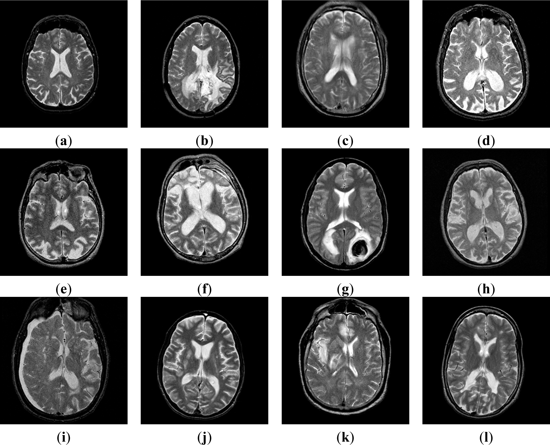
2.1. Benchmark Dataset

Three different benchmark MR image datasets, i.e., Dataset-66, Dataset-160, and Dataset-255, were used for tests in this study. All datasets consist of T2-weighted MR brain images in axial plane and 256 × 256 in-plane resolution, which were downloaded from the website of Harvard Medical School ( http://med.harvard.edu/AANLIB/). Dataset-66 and Dataset-160 were already widely used in brain MR image classification. They consist of abnormal images from seven types of diseases along with normal images. The abnormal brain MR images of the two datasets consists of the following diseases: glioma, meningioma, Alzheimer’s disease, Alzheimer’s disease plus visual agnosia, Pick’s disease, sarcoma, and Huntington’s disease. Das, Chowdhury and Kundu [13] proposed the third dataset “Dataset-255”, which contains 11 types of diseases, among which seven types of diseases are the same as the Dataset-66 and Dataset-160 mentioned before, and four new types of diseases (chronic subdural hematoma, cerebral toxoplasmosis, herpes encephalitis, and multiple sclerosis) were included. Figure 1 shows samples of brain MR images.

The cost of predicting an abnormal brain as normal is severe. It may delay the treatment of the subject. In contrast, the misclassification of a normal brain to an abnormal brain can be corrected by other auxiliary diagnosis techniques.

How to deal with a cost-sensitivity problem? The common methods introduce biases into the error-based classification methods, and they can be divided into following five kinds of solutions [16]:

• Changing the class distribution: resampling, instance reweighting, metacost;
• Boost methods: AdaBoost/Adacost, cost boosting, asymmetric boosting;
• Modifying the learning algorithms: modifying the decision tree, modifying neural networks, modifying SVMs, modifying naive Bayes classifier;
• Direct cost-sensitive learning: Laplace correction, smoothing, curtailment, Platt calibration, and Isotonic regression;
• Other methods: Cost-sensitive CBR, Cost-sensitive specification, Cost-sensitive genetic programming.

In this study, we can access original data, so we change the class distribution at the step of creating the dataset, i.e., we intentionally create three imbalanced datasets, with the aim of solving the cost-sensitivity problem. The imbalanced class distribution [17] can feed into the classifier more abnormal brains, so the classifier is biased to abnormal brains to solve the cost-sensitivity problem.

2.2. CV Setting

Following common conventions and taking advantage of ease of stratified cross validation, 5 × 6-fold stratified cross validation (CV) was used for Dataset-66, and 5 × 5-fold stratified CV was used for the other two datasets.

Table 1. Statistical characteristics and CV setting of the three datasets.

Dataset	Total		Training		Validation		K-Fold
	Normal	Abnormal	Normal	Abnormal	Normal	Abnormal
Dataset-66	18	48	15	40	3	8	6-
Dataset-160	20	140	16	112	4	28	5-
Dataset-255	35	220	28	177	7	43	5-

showed the statistical characteristics and CV settings of the three datasets. In addition, the abnormal brains were set to true and normal brains to false.

We take the Dataset-66 as example, which contains 18 normal and 48 abnormal brains. We use 6-fold stratified cross validation, and assign each fold three normal and eight abnormal brains. Hence, the validation set (one fold) contains three normal and eight abnormal brains, and the training set (the other five folds) contains 15 normal and 40 abnormal ones. Co-registration was not needed because it is not essential. The proposed technique was similar to those used for face recognition, in which some scholars used co-registration [18,19] but others did not use it [20,21]. Moreover, some past publications about abnormal brain detection did not use co-registration [5–15] but they all obtained good results, which were comparable to those obtained employing co-registration [22,23].

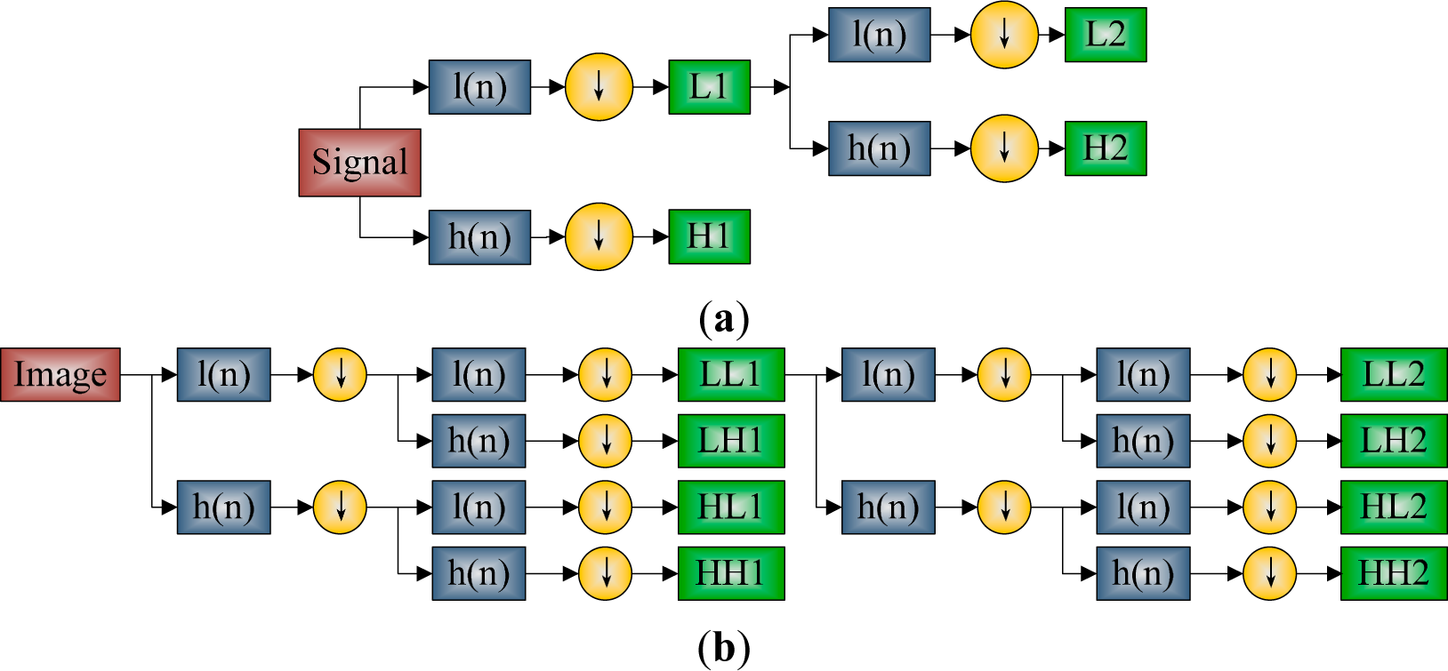
2.3. Discrete Wavelet Transform

The discrete wavelet transform (DWT) is a powerful implementation of the wavelet transform (WT) using the dyadic scales and positions. The fundamental of DWT are introduced as follows: suppose x(t) is a square-integrable function, then the continuous WT of x(t) relative to a given wavelet ψ(t) is defined as [24]:

$$C_{\psi }(f_s,f_t)={\displaystyle {\int }_{-\infty }^{\infty }x(t)\psi (t|f_s,f_t)dt}$$

(1)

where:

$$\psi (t|f_s,f_t)=\frac{1}{\sqrt{f_s}}\psi (\frac{t-f_s}{f_t})$$

(2)

Here, the wavelet ψ(t|f_s, f_t) is calculated from the mother wavelet ψ(t) by translation and dilation: f_s is the scale factor, f_t the translation factor (both real positive numbers), and C the coefficients of WT. There are several different kinds of wavelets which have gained popularity throughout the development of wavelet analysis.

Equation (1) can be discretized by restraining f_s and f_t to a discrete lattice (f_s = 2^f_t & f_s > 0) to give the DWT, which can be expressed as follows:

$$\begin{array}{l}L(n|j,k)=\mathrm{DS}[{\displaystyle {\sum }_{n}x(n)l_j^{*}(n-2^{j}k)}]\\ H(n|j,k)=\mathrm{DS}[{\displaystyle {\sum }_{n}x(n)h_j^{*}(n-2^{j}k)}]\end{array}$$

(3)

Here the coefficients L and H refer to the approximation components and the detail components, respectively. The functions l(n) and h(n) denote the low-pass filter and high-pass filter, respectively. The parameters j and k represent the values of scale and translation factors, respectively. The DS operator means the downsampling.

The above decomposition process can be iterated with successive approximations being decomposed so that one signal is broken down into various levels of resolution [25]. The whole process is called a wavelet decomposition tree. An example of 2-level 1D-DWT is shown in Figure 2a. In applying this technique to MR images, the DWT is applied separately to each dimension. Figure 2b illustrates a schematic diagram of a 2-level 2D-DWT. As a result, there are four subband (LL, LH, HH, HL) images at each scale. The subband LL is used for the next 2D-DWT. The LL subband can be regarded as the approximation component of the image, while the LH, HL, and HH subbands can be regarded as the detailed components of the image. As the level of the decomposition increased, we obtained more compact yet coarser approximation components. Thus, wavelets provide a simple hierarchical framework for interpreting the image information.

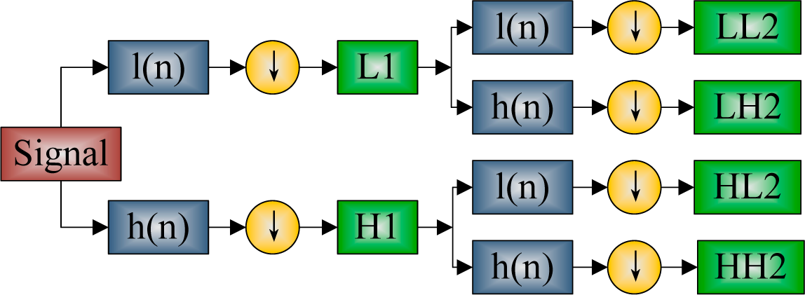
2.4. Discrete Wavelet Packet Transform

DWPT is an extension of DWT, whereby all nodes in the tree structure are allowed to split further at each level of decomposition. In the DWT, each level is calculated by passing only the previous wavelet approximation coefficients through discrete-time low and high pass quadrature mirror filters. However in the DWPT; both the detail and approximation coefficients are decomposed to create the full binary tree (Compare Figure 3 and Figure 2a). Therefore, features can be generated based on approximation and detail coefficients at different levels to obtain more information. The WPT of a signal x(t) is defined as:

$$C_p^{n,j}={\displaystyle {\int }_{-\infty }^{\infty }x(t){\psi }_n(2^{-j}t-p)\mathrm{d}t}$$

(4)

where n is the channel number, j the number of decomposition level (scale parameter), p the position parameter, S the maximum decomposition level, and C the coefficients of WPT. After decomposing signal x(t) by WPT, 2^S sequences can be produced in the S-th level. The fast decomposition equation to next level is:

$$C_k^{2n,j+1}={\displaystyle \sum _{p\in Z}h(p-2k)C_p^{n,j}}$$

(5)

$$C_k^{2n+1,j+1}={\displaystyle \sum _{p\in Z}l(p-2k)C_p^{n,j}}$$

(6)

For j levels of decomposition the DWPT produces 2^j different sets of coefficients as opposed to (3j + 1) sets for the DWT. However; due to the downsampling process the overall number of coefficients of DWPT is still the same of those of DWT; so there is no redundancy.

2.5. Shannon and Tsallis Entropy

Entropy is a statistical measure of randomness, associated with the order of irreversible processes from a traditional point of view. The entropy concept of Boltzmann/Gibbs was redefined as as a measure of uncertainty regarding the information content of a system as Shannon entropy (SE):

$$S=-{\displaystyle \sum _{i=1}^L{p}_i{\log }_2(p_i)}$$

(7)

where i represents the greylevel of reconstructed coefficient, p the probability of greylevel of i, and L the total number of greylevels.

The SE was restricted to the domain of validity of the Boltzmann–Gibbs–Shannon (BGS) statistics, which only described nature when the effective microscopic interactions and the microscopic memory were short ranged [26]. Suppose a physical system can be decomposed into two statistically independent subsystems A and B, the SE has the extensive property (additivity):

$$S(A+B)=S(A)+S(B)$$

(8)

However, for a certain class of physical systems which entail long-range interactions, long time memory, and fractal-type structures, it is necessary to use non-extensive entropy. Tsallis [27] proposed a generalization of BGS statistics, which was termed TE with its form depicted as:

$$S_q=\frac{1-{\displaystyle {\sum }_{i=1}^q{(p_i)}^q}}{q-1}$$

(9)

where the real number q denotes an entropic index that characterizes the degree of non-extensivity. Above expression will meet the SE in the limit q→1. The TE is non-extensive in such a way that for a statistical dependent system [28]. Its entropy is defined with the obey of pseudo-additivity rule:

$$S_q(A+B)=S_q(A)+S_q(B)+(1-q)\times S_q(A)\times S_q(B)$$

(10)

Three different entropies can be defined with regard to different values of q [29]. For q < 1, the TE becomes a sub-extensive entropy where S_q(A + B) < S_q(A) + S_q(B); for q = 1, the TE reduces to an standard extensive entropy where S_q(A + B) = S_q(A) + S_q(B); for q > 1, the TE becomes a super-extensive entropy where S_q(A + B) > S_q(A) + S_q(B).

In this study, TE was employed to extract features from 16 subbands of DWPT coefficients of MR brain images. There were two reasons. First, TE had been successfully applied in brain images [30–32]. Second, the combination of TE and wavelet transform had proven to perform better than either TE or wavelet transform [33–35]. Third, brain images possess long-range interaction and fractal-type structure, because of the self-similarity observed brain structures imaged with a finite resolution. In a word, there are similarities at different spatial scales in brain images, which are more suitable for TE rather than SE.

2.6. Feature Extraction

The features were obtained as the entropies of the DWPT coefficients (see Algorithm 1). We used two kinds of entropies, Shannon entropy and Tsallis entropy, as described above. We compared them in the experiments to find which one was better. Next, we established two classifiers in this study: GEPSVM and kernel GEPSVM.

Algorithm 1:. Feature Extraction

Step 1 Import MR image.

Step 2 Carry out 2-level DWPT decomposition.

Step 3 Calculate the entropy of each subband.

Step 4 Output 16-element entropy vector.

Algorithm 1:. Feature Extraction

Step 1 Import MR image.

Step 2 Carry out 2-level DWPT decomposition.

Step 3 Calculate the entropy of each subband.

Step 4 Output 16-element entropy vector.

2.7. Generalized Eigenvalue Proximal SVM

We consider the task of abnormal brain detection as a binary classification problem. SVM is employed due to its excellent performance reported in the latest literature. In the original SVM, two parallel planes are generated such that each plane is closest to one of two datasets and the two planes are as far apart as possible. Mangasarian and Wild [36] proposed GEPSVM that dropped the parallelism condition on the two hyperplanes, and required each plane be as close as possible to one of the data sets and as far as possible from the other data set. Reports have shown that GEPSVM achieved better classification performance than standard SVM.

Suppose sample data belonging to class 1 and 2 are represented by matrices X₁ and X₂, respectively. GEPSVM aims to determine two nonparallel planes:

$${\mathbf{w}}_1^{T}x-b_1=0\text{and}{\mathbf{w}}_2^{T}x-b_2=0$$

(11)

where the first plane is closest to the points of class 1 and furthest from points in class 2, and the second plane closest to points in class 2 and furthest from points in class 1. To obtain the first plane, we minimize the sum of squares of Euclidean distance between each of the points of class 1 to the plane divided by the squares of Euclidean distance between each of points of class 2 to the plane, which leads to the following optimization problem:

$$({\mathbf{w}}_1,b_1)=\underset{(\mathbf{w},b)\ne 0}{\arg \min }\frac{{\Vert {\mathbf{w}}^T{X}_1-e^{T}b\Vert }^2/{\Vert z\Vert }^2}{{\Vert {\mathbf{w}}^T{X}_2-e^{T}b\Vert }^2/{\Vert z\Vert }^2}$$

(12)

$$z\stackrel{def}{=}\left[\begin{array}{c}\mathbf{w}\\ b\end{array}\right]$$

(13)

Simplifying Equation (12) gives:

$$\underset{(\mathbf{w},b)\ne 0}{\min }\frac{{\Vert {\mathbf{w}}^T{X}_1-e^{T}b\Vert }^2}{{\Vert {\mathbf{w}}^T{X}_2-e^{T}b\Vert }^2}$$

(14)

The Tikhonov regularization term is introduced to reduce the norm of the problem variables (w, b) that determine the first plane in Equation (11):

$$\underset{(\mathbf{w},b)\ne 0}{\min }\frac{{\Vert {\mathbf{w}}^T{X}_1-e^{T}b\Vert }^2+\mathrm{\delta }{\Vert z\Vert }^2}{{\Vert {\mathbf{w}}^T{X}_2-e^{T}b\Vert }^2}$$

(15)

where δ is a nonnegative Tikhonov factor. Equation (15) becomes the “Rayleigh quotient” of the form:

$$z_1=\arg \underset{z\ne 0}{\min }\frac{z^{T}Gz}{z^{T}Hz}$$

(16)

where G and H are symmetric matrices in ${ℝ}^{(p+1)\times (p+1)}$ as:

$$G\stackrel{def}{=}{\left[\begin{array}{cc}{X}_1& -e\end{array}\right]}^T\left[\begin{array}{cc}{X}_1& -e\end{array}\right]+\mathrm{\delta }I$$

(17)

$$H\stackrel{def}{=}{\left[\begin{array}{cc}{X}_2& -e\end{array}\right]}^T\left[\begin{array}{cc}{X}_2& -e\end{array}\right]$$

(18)

Using the boundedness and stationarity properties of Rayleigh Quotient, solution of (16) is obtained by solving the generalized eigenvalue problem:

$$Gz=\lambda Hz,z\ne 0$$

(19)

where the global minimum of Equation (16) is achieved at an eigenvector z₁ corresponding to the smallest eigenvalue λ_min of Equation (19). Hence, w₁ and b₁ can be obtained through Equation (13), and used to determine the plane in Equation (11). Next, we create another optimization problem analogous to Equation (14) by interchanging the roles of X₁ and X₂. The eigenvector z₂* corresponding to the smallest eigenvalue of the second generalized eigenvalue problem will yield the second plane which is close to points of class 2.

2.8. Kernel Technique

Traditional SMVs constructed a hyperplane to classify data, so they cannot deal with classification problems in which the different types of data are located at different sides of a hypersurface; hence the kernel strategy is applied to GEPSVM in this study. Readers can refer to Section 3 in [36] for a detailed description. From another point of view, the kernel technique allows one to fit the hyperplane in a transformed feature space. The transformation may be nonlinear and the transformed space higher dimensional; thus though the classifier is a hyperplane in the higher-dimensional feature space, it may be nonlinear in the original input space. RBF was chosen in this study due to its excellent performance reported in many literatures.

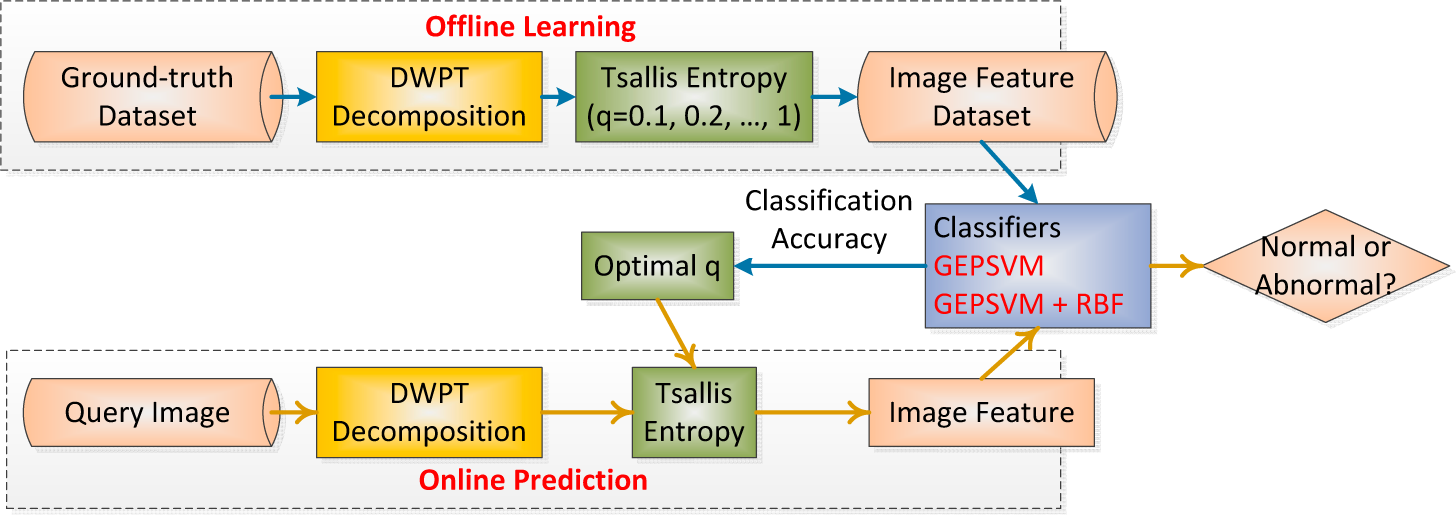
2.9. Implementation of the Proposed Method

The aim of this study was to develop an automatic MR brain image classification system with high classification accuracy. The proposed system consists of three different stages (Figure 4): DWPT decomposition, entropy calculation, and classification. The implementation of the proposed system is two-fold (Algorithm 2): offline learning with the aim of training the classifier, and online prediction with the aim of predict normal/abnormal labels for subjects. Particularly, we varied the value of q from 0.1 to 1 with increment of 0.1, and record the corresponding classification accuracy to select the optimal value of q.

Algorithm 2:. Pseudocodes of the proposed system.

Phase I: Offline learning (users are scientists)
Step 1.	Feature Extraction: Users decompose images by DWPT, and extract Tsallis entropies from all subbands
Step 2.	Classifier Training: The set of features along with the corresponding labels, were used to train the classifier. 10 repetition of K-fold stratified CV was employed for get the out-of-sample evaluation
Step 3.	Evaluation: Report the classification performance.
Step 3.	Parameter Selection: Above three steps iterated with q varies from 0.1 to 1 with increment of 0.1. Select the optimal q that corresponds to the highest classification accuracy.
	Phase II: Online prediction (users are doctors and radiologists)
Step 1.	Feature Extraction: Users presented to the system the query image to be classified. Its feature was obtained as in the offline learning phase.
Step 2.	Predict: Input the features of the query image to previously trained classifier. The classifier labeled the input query image as normal or abnormal.

Algorithm 2:. Pseudocodes of the proposed system.

Phase I: Offline learning (users are scientists)
Step 1.	Feature Extraction: Users decompose images by DWPT, and extract Tsallis entropies from all subbands
Step 2.	Classifier Training: The set of features along with the corresponding labels, were used to train the classifier. 10 repetition of K-fold stratified CV was employed for get the out-of-sample evaluation
Step 3.	Evaluation: Report the classification performance.
Step 3.	Parameter Selection: Above three steps iterated with q varies from 0.1 to 1 with increment of 0.1. Select the optimal q that corresponds to the highest classification accuracy.
	Phase II: Online prediction (users are doctors and radiologists)
Step 1.	Feature Extraction: Users presented to the system the query image to be classified. Its feature was obtained as in the offline learning phase.
Step 2.	Predict: Input the features of the query image to previously trained classifier. The classifier labeled the input query image as normal or abnormal.

2.10. Evaluation

The experiments were carried out on an IBM platform with a 3 GHz core i3 processor and 8 GB RAM, running under the Windows 7 operating system. The algorithm was in-house developed via Matlab 2014a (The Mathworks, Natick, MA, USA).

We designed four experimental tasks in this study. First, we made a visual comparison between DWT and DWPT. A 2-level Haar wavelet was used. Second, we tested the four proposed diagnosis methods:

• (i) DWPT + SE + GEPSVM;
• (ii) DWPT + TE + GEPSVM;
• (iii) DWPT + SE + GEPSVM + RBF;
• (iv) DWPT + TE + GEPSVM + RBF;

We compared them with state-of-the-art methods. Third, we analyzed the computation time for every step of offline learning and online prediction. Finally, we show how to set the optimal parameter q.

3. Experimental Results

3.1. DWPT Result

First, we carried out both DWT and DWPT on a normal and AD MR brain image, respectively. A 2-level Haar wavelet was utilized.

Figure 5a,d show a normal brain MR image and an AD brain MR image. Figure 5b,e show the corresponding 2-level DWT decomposition result, compared with the 2-level DWPT decomposition results shown in Figure 5c,f. Pseudocolor (pink colormap) was added for a clear view.

3.2. Classification Comparison

We compared the proposed four diagnosis methods (viz., the combination of DWPT, two entropy methods, and two classifiers), with state-of-the-art methods (DWT+SOM [5], DWT+SVM [5], DWT + SVM + POLY [5], DWT + SVM + RBF [5], DWT + PCA + FP-ANN [7], DWT + PCA + KNN [7], DWT + PCA + SVM [11], DWT + PCA + SVM + HPOL [11], DWT + PCA + SVM + IPOL [11], DWT + PCA + SVM + GRB [11], DWT + SE + SWP + PNN [12], and RT + PCA + LS-SVM [13]), on the basis of averaging the results of 10 repetition of either 5-fold or 6-fold stratified CV. The comparison results are shown in

Table 2. Classification comparison.

		Dataset-66	Dataset-160	Dataset-255
Existing Approaches [13] (5 Repetitions)	DWT+SOM [5]	94.00	93.17	91.65
	DWT+SVM [5]	96.15	95.38	94.05
	DWT + SVM + POLY [5]	98.00	97.15	96.37
	DWT + SVM + RBF [5]	98.00	97.33	96.18
	DWT + PCA + FP-ANN [7]	97.00	96.98	95.29
	DWT + PCA + KNN [7]	98.00	97.54	96.79
	DWT + PCA + SVM [11]	96.01	95.00	94.29
	DWT + PCA + SVM + HPOL [11]	98.34	96.88	95.61
	DWT + PCA + SVM + IPOL [11]	100.00	98.12	97.73
	DWT + PCA + SVM + GRB [11]	100.00	99.38	98.82
	DWT + SE + SWP + PNN [12]	100.00	99.88	98.90
	RT + PCA + LS-SVM [13]	100.00	100.00	99.39
Proposed approaches (10 repetitions)	DWPT + SE + GEPSVM	99.85	99.62	98.78
	DWPT + TE + GEPSVM	100.00	100.00	99.33
	DWPT + SE + GEPSVM + RBF	100.00	99.88	99.33
	DWPT + TE + GEPSVM + RBF	100.00	100.00	99.53

, where the existing approaches are extracted from [13] and the “DWT + SE + SWP + PNN” method was calculated by us. Reference [13] used five repetitions, while our experiment used 10 repetitions to get a more robust evaluation result. The term q was assigned a value of 0.8 (See Section 3.3). The regularization constant and kernel parameter were obtained via grid-search, which trained the classifier with each pair in the Cartesian product of the two sets (10, 100, 1000) and (0.1, 0.2, 0.5, 1.0, 2.0).

The detailed evaluations of one repetition of the proposed DWPT + TE + GEPSVM + RBF method are listed in

Table 3. One repetition of DWPT + TE + GEPSVM + RBF method.

Dataset	Sensitivity	Specificity	Precision	Accuracy
Dataset-66	100.00	100.00	100.00	100.00
Dataset-160	100.00	100.00	100.00	100.00
Dataset-255	100.00	97.14	99.55	99.61

.

3.3. Setting of Parameter q

A problem arose with how to determine the optimal value of q? Obviously q should be less than 1 since the brain is a subextensive system that consists of complex areas and tissues. Then, we varied the value of q from 0.1 to 1 with increment of 0.1, and recorded the average classification accuracy over 10 repetitions of Dataset-255 by two proposed methods “DWPT + TE + GEPSVM” and “DWPT + TE + GEPSVM + RBF”. The results are shown in Figure 6 and

Table 4. Detailed Data of Figure 6.

Method	q = 0.1	0.2	0.3	0.4	0.5	0.6	0.7	0.8	0.9	1
DWPT + TE + GEPSVM	99.02	99.02	99.06	99.06	99.18	99.11	99.29	99.33	98.94	98.82
DWPT + TE + GEPSVM + RBF	99.29	99.33	99.33	99.41	99.37	99.37	99.41	99.53	99.49	99.33

.

3.4. Computational Burden Analysis

Computation time is another important factor to evaluate a classifier.

Table 5. Computation time analysis based on Dataset-255.

	Step	Time (s)
Offline Learning	DWPT decomposition	4.0565
	Entropy calculation	3.4961
	Classifier training	0.8904
Online Prediction	DWPT decomposition	0.0817
	Entropy calculation	0.0213
	Brain classification	0.0029

records the time consumed of each step using Dataset-255. For the offline learning phase, the three procedures, i.e., DWPT, Entropy calculation, and classifier training, took 4.0565 s, 3.4961 s, and 0.8904 s, respectively. For the online learning phase, the three procedures, i.e., DWPT, Entropy calculation, and brain classification, took 0.0817 s, 0.0213 s, and 0.0029 s, respectively.

3.5. Discussion

3.5.1. Discussion of Results

From Table 2, the RBF kernel was effective, after comparing the classification result of “DWPT + TE + GEPSVM + RBF” with “DWPT + TE + GEPSVM”, and comparing “DWPT + SE + GEPSVM + RBF” with “DWPT + SE + GEPSVM”. We found that techniques with RBF kernel obtained higher accuracy those without RBF. This finding aligns with past publications [5,11].

Another finding was that TE was superior to traditional SE, after comparing the result of “DWPT + TE + GEPSVM” with “DWPT + SE + GEPSVM”, and comparing the result of “DWPT + TE + GEPSVM + RBF” with “DWPT + SE + GEPSVM + RBF”. The reason is because Tsallis entropy is a generalization of traditional SE [37]. Brain MR images showed the presence of correlation between pixels of the same tissue, so they were especially suitable to be represented by TE.

Finally, “DWPT + TE + GEPSVM + RBF” performed the best among the four proposed diagnosis methods, obtaining classification accuracies of 100.00%, 100.00%, and 99.53% for the three datasets. The also proved the effectiveness of GEPSVM, which dropped the parallelism condition, leading to a more flexible hyperplane construction. The next is RT + PCA + LS-SVM [13] that achieved 100.00%, 100.00%, and 99.39% for the three datasets. Table 4 showed the proposed DWPT + TE + GEPSVM + RBF outperformed not only three other proposed diagnosis methods, but also the state-of-the-art algorithms of MR brain classification.

The results in Table 3 showed that the DWPT + TE + GEPSVM + RBF performed perfectly on either Dataset-66 or Dataset-160. For Dataset-255, its sensitivity was 100%, specificity was 97.14%, precision was 99.55%, and accuracy was 99.61%. This corresponded to the situation where one normal brain image was mislabeled as abnormal while all abnormal brains were recognized correctly. Note that Table 4 were obtained based on ten repetitions, hence, the accuracies of Tables 2 and 3 were not coherent.

The curves in Figure 6 and the data in Table 4 showed the value of q produced slight but discernible effects on the average classification accuracy. As q increased from 0.1 to 0.8, the average classification accuracy increased gradually until the point where q = 0.8, which produced the highest classification accuracy. Then, the curves decreased sharply when q increased from 0.8 to 0.1. The Tsallis entropy degraded to Shannon entropy when q equals to 1. It was obvious that introducing Tsallis entropy did improve the classification performance.

This result (q = 0.8) was identical to the conclusions of Sturzbecher et al. [38] and Cabella et al. [39]. Diniz et al. [40] on the other hand found that q was best as 0.2 for CSF, 0.1 for white matter and 1.5 for gray matter. For this study, we had to assign a single value of q on the whole image, hence, our result of 0.8 can be regarded as an average of best q values of CSF, white matter and gray matter.

From Table 5, we can calculate that the offline learning cost totally cost as 4.0565 + 3.4961 + 0.8904 = 8.4430 s, whereas the computer required only 0.0817 + 0.0213 + 0.0029 = 0.1059 s for online prediction. The offline learning takes much more time than online prediction, because offline learning needs to operate with 255 images whereas online prediction just focuses on one query image. In addition, the classifier training in the offline learning phase had already obtained the weights/biases of the classifier, so the brain classification in the online prediction phase directly used a trained classifier to obtain the output.

DWPT takes more time than DWT on average, because it needs to decompose not only the approximation coefficients, but also the detailed coefficients. In spite of this, the computation time in practical use (online prediction) was 0.1059 s, which was relatively fast and met real-time requirements.

3.5.2. Discussion on the Proposed Method

Revisiting the whole methodology of the proposed CAD system, there were three reasons why we used DWPT, Tsallis entropy, and GEPSVM. First, DWPT can obtain more high-frequency information and more detailed frequency domain information than DWT, which are essentially important in training the classifier. Second, entropy can efficiently represent the complexity and uncertainty of signals. Finally, GEPSVM dropped the parallelism condition required by standard SVM, leading to a more flexible hyperplane construction.

We chose the 2-level Haar wavelet by experience; however, there are other outstanding wavelets such as db and bior series, and other decomposition levels may give better performance. In the future, we expect to develop an algorithm that can automatically determine the optimal wavelet and the optimal decomposition level.

The GEPSVM is an excellent classifier that relaxes the universal requirement that bounding or proximal planes should be parallel in the input space for linear classifier or in the higher dimensional feature space for nonlinear kernel classifier. This study showed its success in the application of MR brain image classification. The nonparallel planes are easily obtained using a single Matlab command that solved the classical generalized eigenvalue problem. The simple program formulation, computational efficiency, and high classification accuracy proved it was an extremely effective algorithm for classification.

TE proved to be better than SE in this study. The setting of value of q still remained a problem, since we performed a rather coarse search by varying its value from the range of 0.1 to 1 with increment of 0.1. The problem belonged to hyperparameter optimization, which needs to choose a set of parameters for a learning algorithm with the goal of optimizing the algorithm’s performance. Some other hyperparameter optimization techniques will be used like random search, Bayesian optimization, etc.

A limitation was that the classifier was machine-oriented not human-oriented. Although machine-oriented classifiers yielded better classification performance than human-oriented classifiers, technicians cannot understand or interpret what the weights/biases of the classifier mean, which limited its usage in reality. Another limitation was the computation time of DWPT, which took the most time during either the offline learning stage or online prediction stage. In the future we will try to use fast algorithms to implement DWPT.

4. Conclusions and Future Research

In this study, we treated the abnormal brain detection as a binary classification problem. To solve it, we proposed to use DWPT to replace the traditional DWT method, and we proposed two entropy methods (SE and TE), and two classifiers (GEPSVM with and without RBF kernel), with the aim of developing an automatic classifier for MR brain images. The experiments showed the proposed “DWPT + TE + GEPSVM + RBF” diagnosis method yielded superior performance to not only the other three proposed methods (DWPT + SE + GEPSVM, DWPT + TE + GEPSVM, and DWPT + SE + GEPSVM + RBF) but also current state-of-the-art methods.

The contributions of this study center in the following five aspects: (i) we used DWPT that offered better information description than DWT; (ii) we used TE to extract entropy features from DWPT coefficients, and proved TE was better than SE; (iii) we used GEPSVM that had better generalization ability, and proved it got higher classification accuracy than SVM; (iv) we proved the kernel technique was effective; and (v) we proved the proposed “DWPT + TE + GEPSVM + RBF” methods achieved better classification than existing state-of-the-art methods.

Future work should focus on the following four aspects: (i) we will include other imaging techniques, such as DTI and MRSI [41]; (ii) the classification performance may increase by using other advanced variants of SVM; (iii) we will check the effects produced by other wavelet families, different decomposition levels, and different kernel methods; and (iv) we will test other hyperparameter optimization techniques.

References

1. Goh, S.; Dong, Z.; Zhang, Y.; DiMauro, S.; Peterson, B.S. Mitochondrial dysfunction as a neurobiological subtype of autism spectrum disorder: Evidence from brain imaging. JAMA Psychiatry 2014, 71, 665–671. [Google Scholar]
2. Zhang, Y.; Wang, S.; Ji, G.; Dong, Z. Exponential wavelet iterative shrinkage thresholding algorithm with random shift for compressed sensing magnetic resonance imaging. IEEJ Trans. Electr. Electron. Eng. 2015, 10, 116–117. [Google Scholar]
3. Zhang, Y.D.; Dong, Z.C.; Ji, G.L.; Wang, S.H. An improved reconstruction method for CS-MRI based on exponential wavelet transform and iterative shrinkage/thresholding algorithm. J. Electromagn. Waves Appl 2014, 28, 2327–2338. [Google Scholar]
4. Levman, J.E.D.; Warner, E.; Causer, P.; Martel, A.L. A Vector machine formulation with application to the computer-aided diagnosis of breast cancer from DCE-MRI screening examinations. J. Digit. Imaging 2014, 27, 145–151. [Google Scholar]
5. Chaplot, S.; Patnaik, L.M.; Jagannathan, N.R. Classification of magnetic resonance brain images using wavelets as input to support vector machine and neural network. Biomed. Signal Process. Control 2006, 1, 86–92. [Google Scholar]
6. Maitra, M.; Chatterjee, A. A Slantlet transform based intelligent system for magnetic resonance brain image classification. Biomed. Signal Process. Control 2006, 1, 299–306. [Google Scholar]
7. El-Dahshan, E.S.A.; Hosny, T.; Salem, A.B.M. Hybrid intelligent techniques for MRI brain images classification. Digit. Signal Process 2010, 20, 433–441. [Google Scholar]
8. Zhang, Y.; Wu, L.; Wang, S. Magnetic resonance brain image classification by an improved artificial bee colony algorithm. Progress Electromagn. Res. 2011, 116, 65–79. [Google Scholar]
9. Zhang, Y.; Dong, Z.; Wu, L.; Wang, S. A hybrid method for MRI brain image classification. Expert Syst. Appl 2011, 38, 10049–10053. [Google Scholar]
10. Ramasamy, R.; Anandhakumar, P. Brain tissue classification of MR images using fast Fourier transform based expectation-maximization Gaussian mixture model. In Advances in Computing and Information Technology; Springer: Berlin/Heidelberg, Germany, 2011; pp. 387–398. [Google Scholar]
11. Zhang, Y.; Wu, L. An MR brain images classifier via principal component analysis and Kernel support vector machine. Progress Electromagn. Res. 2012, 130, 369–388. [Google Scholar]
12. Saritha, M.; Paul Joseph, K.; Mathew, A.T. Classification of MRI brain images using combined wavelet entropy based spider web plots and probabilistic neural network. Pattern Recognit. Lett. 2013, 34, 2151–2156. [Google Scholar]
13. Das, S.; Chowdhury, M.; Kundu, M.K. Brain MR image classification using multiscale geometric analysis of ripplet. Progress Electromagn. Res. 2013, 137, 1–17. [Google Scholar]
14. Kalbkhani, H.; Shayesteh, M.G.; Zali-Vargahan, B. Robust algorithm for brain magnetic resonance image (MRI) classification based on GARCH variances series. Biomed. Signal Process. Control 2013, 8, 909–919. [Google Scholar]
15. Zhang, Y.; Wang, S.; Dong, Z. Classification of Alzheimer disease based on structural Magnetic resonance imaging by Kernel support vector machine decision tree. Progress Electromagn. Res. 2014, 144, 171–184. [Google Scholar]
16. Qin, Z.X.; Zhang, C.Q.; Wang, T.; Zhang, S.C. Cost sensitive classification in data mining. Adv. Data Min. Appl 2010, Pt I 2010, 6440, 1–11. [Google Scholar]
17. Zhang, Y.; Wang, S.; Phillips, P.; Ji, G. Binary PSO with mutation operator for feature selection using decision tree applied to spam detection. Knowl.-Based Syst. 2014, 64, 22–31. [Google Scholar]
18. Kong, Y.H.; Zhang, S.M.; Cheng, P.Y. Super-resolution reconstruction face recognition based on multi-level FFD registration. Optik 2013, 124, 6926–6931. [Google Scholar]
19. Liao, S.; Shen, D.G.; Chung, A.C.S. A Markov random field groupwise registration framework for face recognition. IEEE Trans. Pattern Anal. Mach. Intell. 2014, 36, 657–669. [Google Scholar]
20. Shi, J.G.; Qi, C. From local geometry to global structure: Learning latent subspace for low-resolution face image recognition. IEEE Signal Process. Lett. 2015, 22, 554–558. [Google Scholar]
21. Fan, Z.Z.; Ni, M.; Zhu, Q.; Liu, E. Weighted sparse representation for face recognition. Neurocomputing 2015, 151, 304–309. [Google Scholar]
22. Ribbens, A.; Hermans, J.; Maes, F.; Vandermeulen, D.; Suetens, P.; Alzheimers Dis, N. Unsupervised segmentation, clustering, and groupwise registration of heterogeneous populations of brain MR images. IEEE Trans. Med. Imaging 2014, 33, 201–224. [Google Scholar]
23. Schwarz, D.; Kasparek, T. Brain morphometry of MR images for automated classification of first-episode schizophrenia. Inf. Fusion 2014, 19, 97–102. [Google Scholar]
24. Fang, L.; Wu, L.; Zhang, Y. A novel demodulation system based on continuous wavelet transform. Math. Probl. Eng. 2015, 2015. [Google Scholar] [CrossRef]
25. Zhou, R.; Bao, W.; Li, N.; Huang, X.; Yu, D. Mechanical equipment fault diagnosis based on redundant second generation wavelet packet transform. Digit. Signal Process 2010, 20, 276–288. [Google Scholar]
26. Campos, D. Real and spurious contributions for the Shannon, Rényi and Tsallis entropies. Physica A 2010, 389, 3761–3768. [Google Scholar]
27. Tsallis, C. Nonadditive entropy: The concept and its use. Eur. Phys. J. A. 2009, 40, 257–266. [Google Scholar]
28. Zhang, Y.; Wu, L. Optimal multi-level thresholding based on maximum Tsallis entropy via an artificial bee colony approach. Entropy 2011, 13, 841–859. [Google Scholar]
29. Tsallis, C. The nonadditive entropy S-q and its applications in physics and elsewhere: Some remarks. Entropy 2011, 13, 1765–1804. [Google Scholar]
30. Amaral-Silva, H.; Wichert-Ana, L.; Murta, L.O.; Romualdo-Suzuki, L.; Itikawa, E.; Bussato, G.F.; Azevedo-Marques, P. The superiority of Tsallis entropy over traditional cost functions for brain MRI and SPECT registration. Entropy 2014, 16, 1632–1651. [Google Scholar]
31. Venkatesan, A.S.; Parthiban, L. A Novel nature inspired fuzzy Tsallis entropy segmentation of magnetic resonance images. Neuroquantology 2014, 12, 221–229. [Google Scholar]
32. Khader, M.; Ben Hamza, A. Nonrigid image registration using an entropic similarity. IEEE Trans. Inf. Technol. Biomed. 2011, 15, 681–690. [Google Scholar]
33. Hussain, M. Mammogram enhancement using lifting dyadic wavelet transform and normalized Tsallis entropy. J. Comput. Sci. Technol 2014, 29, 1048–1057. [Google Scholar]
34. Liu, Z.G.; Hu, Q.L.; Cui, Y.; Zhang, Q.G. A new detection approach of transient disturbances combining wavelet packet and Tsallis entropy. Neurocomputing 2014, 142, 393–407. [Google Scholar]
35. Chen, J.K.; Li, G.Q. Tsallis wavelet entropy and its application in power signal analysis. Entropy 2014, 16, 3009–3025. [Google Scholar]
36. Mangasarian, O.L.; Wild, E.W. Multisurface proximal support vector machine classification via generalized eigenvalues. IEEE Trans. Pattern Anal. Mach. Intell 2006, 28, 69–74. [Google Scholar]
37. Tsallis, C. An introduction to nonadditive entropies and a thermostatistical approach to inanimate and living matter. Contemp. Phys. 2014, 55, 179–197. [Google Scholar]
38. Sturzbecher, M.J.; Tedeschi, W.; Cabella, B.C.T.; Baffa, O.; Neves, U.P.C.; de Araujo, D.B. Non-extensive entropy and the extraction of BOLD spatial information in event-related functional MRI. Phys. Med. Biol 2009, 54, 161–174. [Google Scholar]
39. Cabella, B.C.T.; Sturzbecher, M.J.; de Araujo, D.B.; Neves, U.P.C. Generalized relative entropy in functional magnetic resonance imaging. Physica A 2009, 388, 41–50. [Google Scholar]
40. Diniz, P.R.B.; Murta, L.O.; Brum, D.G.; de Araujo, D.B.; Santos, A.C. Brain tissue segmentation using q-entropy in multiple sclerosis magnetic resonance images. Braz. J. Med. Biol. Res. 2010, 43, 77–84. [Google Scholar] [Green Version]
41. Dong, Z.; Zhang, Y.; Liu, F.; Duan, Y.; Kangarlu, A.; Peterson, B.S. Improving the spectral resolution and spectral fitting of 1H MRSI data from human calf muscle by the SPREAD technique. NMR Biomed. 2014, 27, 1325–1332. [Google Scholar]
Figure 1. Samples of brain MR images. (a) Normal brain; (b) Glioma; (c) Meningioma; (d) AD; (e) AD with visual agnosia; (f) Pick’s disease; (g) Sarcoma; (h) Huntington’s disease; (i) Chronic subdural hematoma; (j) Cerebral toxoplasmosis; (k) Herpes encephalitis; (l) Multiple sclerosis.
Entropy 17 01795f1
Figure 2. Schematic Diagram of DWT. The downward arrow denotes DS operation. (a) 2-level 1D-DWT; (b) 2-level 2D-DWT.
Entropy 17 01795f2
Figure 3. Flowchart of a 2-level 1D-DWPT.
Entropy 17 01795f3
Figure 4. Flowchart of the proposed system.
Entropy 17 01795f4
Figure 5. Decomposition comparison between DWT and DWPT. (a) normal brain; (b) 2-level DWT of normal brain; (c) 2-level DWPT of normal brain; (d) AD brain; (e) 2-level DWT of AD brain; (f) 2-level DWPT of AD brain.
Entropy 17 01795f5
Figure 6. Effect of q value on classification accuracy (q = 1 corresponds to SE).
Entropy 17 01795f6