New Patterns in Steady-State Chemical Kinetics: Intersections, Coincidences, Map of Events (Two-Step Mechanism)

Abstract

New patterns of steady-state chemical kinetics for continuously stirred-tank reactors (CSTR) have been found, i.e., intersections, maxima and coincidences, for two-step mechanism A↔B→C. There were found elegant analytical relationships for characteristics of these patterns (space times, values of concentrations and rates) allowing kinetic parameters to be easily determined. It was demonstrated that for the pair of species involved into the irreversible reaction (B and C), the space time of their corresponding concentration dependence intersection is invariant and does not depend on the initial conditions of the system. Maps of patterns are presented for visualization of their combinations and ranking in space time, and values of concentration and rates.

1. Introduction

Recently new properties of simplest chemical systems, linear and non-linear, have been discovered [1,2,3,4,5,6,7,8,9]. It was found that some simple chemical reactions with commensurate parameters exhibit previously unknown interesting temporal behavior features. Different classes of new patterns have been described for the description of non-steady concentration evolutions in batch reactors (BR) and, identically, for longitudinal profiles in plug-flow reactors (PFR), and for Temporal-Analysis-of-Products (TAP) reactors; in particular, (1) time invariances in reciprocal kinetic experiments, (2) intersections and (3) coincidences. All analyzed models presented sets of differential equations, either ordinary (BR- or PFR-models) or partial (TAP-reactor models).

Presently only one class of typical models of chemical reactors was remained out of such pattern analysis, viz. algebraic models of open reactors with perfect mixing, i.e., steady-state continuously-stirred tank reactors (CSTRs).

1.1. Time Invariances in Reciprocal Kinetic Experiments

In experiments performed in BR or PFR or TAP-reactors from symmetrical initial conditions, certain mixed quotient-like functions of selected concentrations from both experiments are always equal to the equilibrium constant of the reaction.

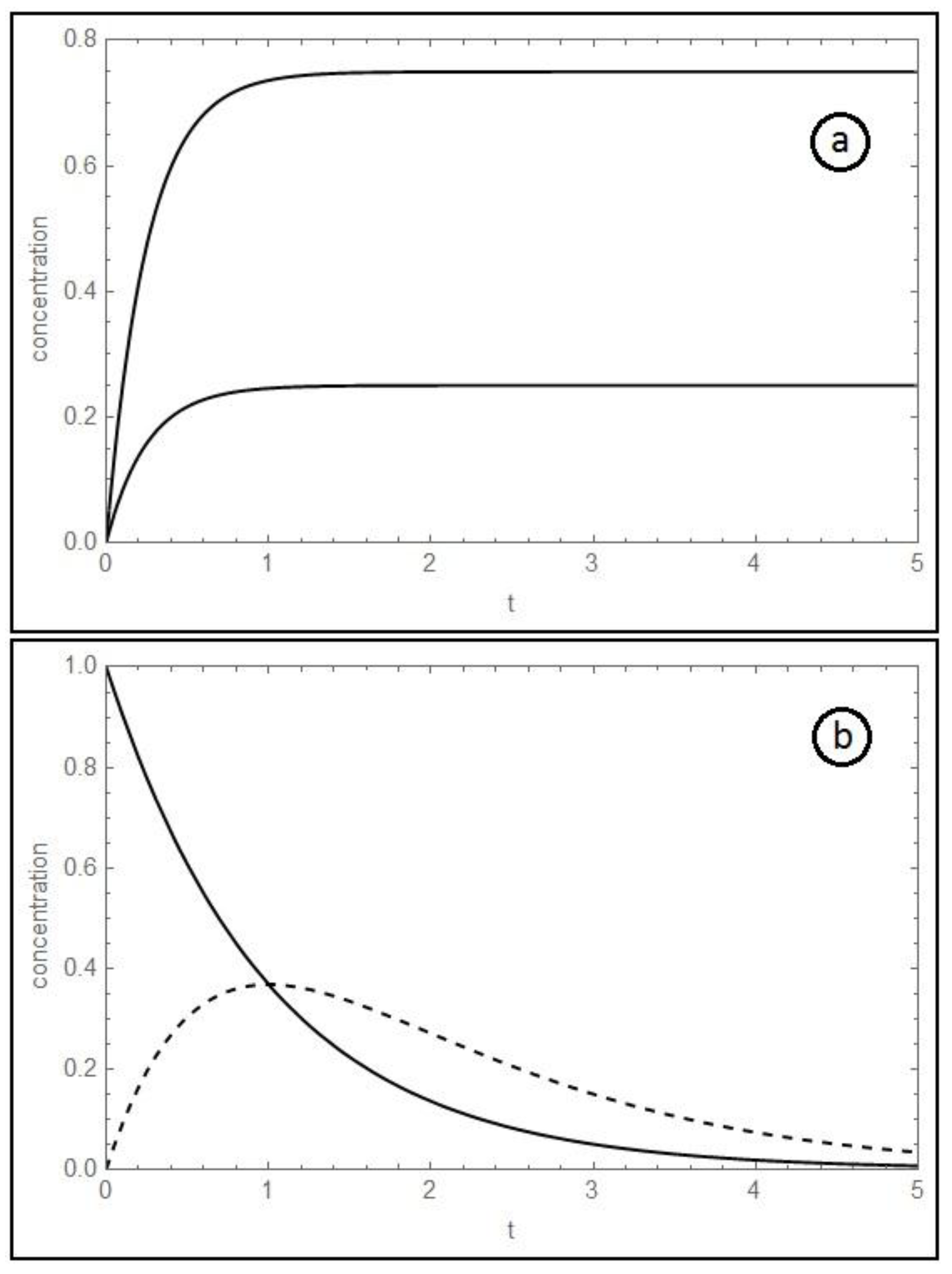
The first-order reversible reaction A↔B presents the simplest example of this phenomenon. To demonstrate it, we can design two different, reciprocal experiments, regarding the initial concentration of the two chemical species involved. In the first, we record the concentration-time profile of B produced from pure A, ${\text{C}}_{{\text{B}}_{\text{A}}}\left(\text{t}\right)$. In the second experiment we record the temporal evolution of the concentration of A produced from pure B, ${\text{C}}_{{\text{A}}_{\text{B}}}\left(\text{t}\right)$. The composition of A and B will be the same at the end of both experiments, when equilibrium is achieved at t→∞, i.e., K_eq = k⁺/k⁻ = C_B(t→∞) / C_A(t→∞), where K_eq is the equilibrium constant of the reversible reaction, and k⁺ and k⁻ the first-order kinetic constants of the forward and backward single reactions, respectively. Therefore, for this example a remarkable feature occurs: the ratio of concentrations ${\text{C}}_{{\text{B}}_{\text{A}}}\left(\text{t}\right)$/${\text{C}}_{{\text{A}}_{\text{B}}}\left(\text{t}\right)$ is constant in time and equal to the equilibrium constant K_eq at any time, not only under equilibrium conditions (see Figure 1a, Yablonsky et al. [1]).

A general theory of this phenomenon was presented in [2], based on the property of linear or linearized kinetics with microreversibility, dx/dt = Kx, that the kinetic operator, K, is symmetric in the entropic inner product. This form of Onsager’s reciprocal relations implies that the shift in time, exp (Kt), is also a symmetric operator. It generates the reciprocity relations between the kinetic curves. For example, for the Master equation, if we start the process from the i-th pure state and measure the probability p_j(t) of the j-th state (i not equal j), and similarly measure p_j(t) for the process which starts at the j-th pure state, then, the ratio of both probabilities, p_j(t) / p_i(t) will be constant in time and coincides with the ratio of equilibrium probabilities. Therefore, in such reciprocal experiments the ratio of concentrations will be governed by a thermodynamic relationship if the corresponding substances are related to the linear sub-mechanism.

Figure 1. (a) Temporal evolution of B_A (upper solid curve) and A_B (lower solid curve), for the system A↔B; (k⁺, k⁻) = (3, 1 s⁻¹). The ratio B_A/A_B is always constant, and equal to K_eq = k⁺/k⁻. (b) Temporal evolution of B_A (solid curve) and C_A (dashed curve), for the system A→B→C; k₁ = k₂ = 1 s⁻¹. See refs. [1] and [3].

Figure 1. (a) Temporal evolution of B_A (upper solid curve) and A_B (lower solid curve), for the system A↔B; (k⁺, k⁻) = (3, 1 s⁻¹). The ratio B_A/A_B is always constant, and equal to K_eq = k⁺/k⁻. (b) Temporal evolution of B_A (solid curve) and C_A (dashed curve), for the system A→B→C; k₁ = k₂ = 1 s⁻¹. See refs. [1] and [3].

Similar reciprocal relations between kinetic curves have been found in pulse-response TAP-studies of the Water-Gas-Shift (WGS) reaction over iron oxide catalyst. These data offered an excellent confirmation within the experimental error.

1.2. Intersections

An intersection of two or more temporal characteristics, for instance, C_A(t) and C_B(t), means that those concentrations can be considered equal at some moment in time, C_A(t) = C_B(t). As well known, phase trajectories do not intersect or merge. Nevertheless, the temporal trajectories may well intersect, or not, and this fact is used as additional source of information.

1.3. Coincidences

A coincidence in time means that at least two special events occur at the same point in time. When two special events occur at the same value of concentration we have a coincidence in value, i.e. C_A(t) = C_B(t). For example, the culmination point of one concentration dependence may coincide with the point at which this dependence intersects with another concentration; or the intersection between three concentration dependences may occur at the same moment in time, i.e., a triple intersection. Some spectacular examples of coincidences for the irreversible consecutive mechanism A→B→C are presented in Figure 1b. At k₁ = k₂, where k₁ and k₂ are the kinetic constants of the first and the second reaction, respectively, the concentration dependence of B_A intersects the concentration dependence of C_A at its peak, and C_A,0/C_{B, max} = e, where C_A,0 is the initial concentration of substance A, and B_max is the maximum concentration of substance B, respectively.

In [7], Constales et al. presented a thorough study of both reciprocal symmetries, times of intersections and concentration values at these points, and coincidences as well for the reaction scheme A↔B→C in a batch reactor.

Summing up, the described new patterns open new possibilities:

(a)

For testing the validity of the corresponding model;

(b)

For estimating the parameters of the model based on the occurrence of patterns;

(c)

For predicting kinetic behavior.

1.4. Goal

The goal of this paper is to reveal the similar patterns related to the steady-state kinetic behavior of reactions in a continuously stirred tank reactor (CSTR). As mentioned, this class of models was still not analyzed regarding the possible new patterns. In comparison with previously analyzed reactor models (models of BR, PFR and TAP-reactor models), CSTR-models are sets of algebraic equations, not differential ones. This creates an additional advantage in obtaining the general analytic relationship for new patterns. Also the CSTR is very convenient in change of control parameters, inlet concentrations and space time controlled by the flow rate. It is assumed that the temperature in the reactor remains constant throughout the reaction, i.e., the isothermal condition is guaranteed. The reader is referred to [7,10] to cover the influence of the temperature on the values of the kinetic coefficients.

1.5. Model

The general form of CSTR models of complex chemical reactions in homogeneous reactors is:

$$\frac{{\text{F}}_{\text{j}}-{\text{F}}_{\text{j},0}}{\text{V}}=\frac{{\text{q}}_{\text{V}}{\text{C}}_{\text{j}}-{\text{q}}_{\text{V},0}{\text{C}}_{\text{j},0}}{\text{V}}={\text{R}}_{\text{j}}={\displaystyle \sum }_{\text{i}}{\text{υ}}_{\text{ij}}{r}_i\text{ j}=1,2\dots \text{n}$$

(1)

where F_j = q_VC_j and F_j,0 = q_V,0C_j,0 [mol∙s⁻¹] are the molar flow rates of the j-th species inside the reactor and its inlet, respectively, C_j and C_j,0 [mol∙m⁻³] are the concentrations of the j-th species inside the reactor and its inlet, respectively, and R_j is its rate of species change [mol∙m⁻³∙s⁻¹] in the course of the i-th reaction. R_j = ${\sum }_{\text{i}}{\text{υ}}_{\text{ij}}{r}_i$, where r_i is the rate of step of complex chemical reaction [mol∙m⁻³∙s⁻¹], v_ij is the stoichiometric coefficient of the j-th species in the i-th step. q_V represent the flow rate in the reactor [m³∙s⁻¹], q_V,0 is the initial flow rate, and V represents the volume of the reactor [m³]. In our case, all reactions will be considered as monomolecular (first-order reactions), and there is no change of volume during each reaction. Consequently, the flow rate q_V = q_V,0, and the space time of the reactive mixture τ can be defined as τ = V/q_V,0, and R_j = (C_j − C_j,0)/τ [10].

For a heterogeneous catalytic reactor, say a heterogeneous catalytic reactor, similarly $\text{τ}=\frac{{\text{v}}_{\text{cat}}}{q_{V,0}}$, where v_cat is the catalyst volume [m³]. In many cases, $\text{τ}=\frac{{\text{S}}_{\text{cat}}}{q_{V,0}}$, where S_cat is the active catalyst surface [m²]. Corresponding to these dimensions, the chemical rate has to have the dimension [mol·m⁻²·s⁻¹].

The best known and most studied event of reacting chemical mixture is reaching equilibrium. Based on the equilibrium chemical composition, it is easy to find equilibrium constants of all steps of the assumed mechanism taking into account the principle of detailed equilibrium (PDE) if necessary. By definition, this can be done only if all steps of the mechanism are reversible. However using the equilibrium composition, it is impossible to determine kinetic parameters of separate reactions even applying the PDE. In contrary to the described traditional approach, we are going to present a method for determining the kinetic parameters of separate reactions, both reversible and irreversible, based on characteristics of special events (patterns), in particular times of intersections and maxima of concentrations dependences, and values of concentrations and rates at temporal points of these events.

We will try to select a class of chemical mechanism that is as wide as possible for the application of this method. Then, we will illustrate this method using as an example the multi-step mechanism which includes both reversible and irreversible mechanism. We consider such reversible-irreversible mechanism very typical for chemistry of complex reactions. Rigorously speaking, all chemical reactions are reversible. However, in reality most of important reactions (reactions of hydrocarbon oxidation, hydrogen combustion, enzyme reactions) are generally irreversible. At the same time, some of the reactions included into the complex mechanism are reversible, e.g., primary generation of H radicals in hydrogen combustion, adsorption of the substrate in the Michaelis-Menten enzyme mechanism, etc. That is why this reversible-irreversible mechanism is chosen as a subject for studies in our paper.

As an example, we are using a two-step consecutive reaction A ↔ B → C, where the first reaction is reversible and the second one is irreversible. For this mechanism, the CSTR model is:

$$\{\begin{array}{c}\frac{{\text{C}}_{\text{A}}\left(\text{τ}\right)-{\text{C}}_{\text{A}}\left(0\right)}{\text{τ}}={\text{R}}_{\text{A}}\left(\text{τ}\right)=-{\text{k}}_1^{+}{\text{C}}_{\text{A}}\left(\text{τ}\right)+{\text{k}}_1^{-}{\text{C}}_{\text{B}}\left(\text{τ}\right)\\ \frac{{\text{C}}_{\text{B}}\left(\text{τ}\right)-{\text{C}}_{\text{B}}\left(0\right)}{\text{τ}}={\text{R}}_{\text{B}}\left(\text{τ}\right)={\text{k}}_1^{+}{\text{C}}_{\text{A}}\left(\text{τ}\right)-({\text{k}}_1^{+}+{\text{k}}_2){\text{C}}_{\text{B}}\left(\text{τ}\right)\\ \frac{{\text{C}}_{\text{C}}\left(\text{τ}\right)-{\text{C}}_{\text{C}}\left(0\right)}{\text{τ}}={\text{R}}_{\text{C}}\left(\text{τ}\right)={\text{k}}_2{\text{C}}_{\text{B}}\left(\text{τ}\right)\end{array}$$

(2)

where τ is the space time, C_i(τ) and C_i(0) are the space time-dependent concentration and the initial concentration on the reactor of the i species, respectively. R_i(τ) is the rate of change of the i species. The forward and backward kinetic constants for the first reversible reaction are k₁⁺ and k₁⁻, respectively, and k₂ the kinetic constant of the second, irreversible reaction.

The solution of the kinetic model described in (2) is obtained by isolating the C_i(τ) terms, and, assuming $\text{κ}=1+\left({\text{k}}_1^{+}+{\text{k}}_1^{-}+{\text{k}}_2\right)\text{τ}+{\text{k}}_1^{+}{\text{k}}_2{\text{τ}}^2$, the corresponding concentration-space time expressions are simple, as follows:

$$\{\begin{array}{c}{\text{C}}_{\text{A}}\left(\text{τ}\right)=\frac{{\text{C}}_{\text{A}}\left(0\right)(1+{\text{k}}_2\text{τ})+({\text{C}}_{\text{A}}\left(0\right)+{\text{C}}_{\text{B}}\left(0\right)){\text{k}}_1^{-}\text{τ}}{\text{κ}}\\ {\text{C}}_{\text{B}}\left(\text{τ}\right)=\frac{({\text{C}}_{\text{A}}\left(0\right)+{\text{C}}_{\text{B}}\left(0\right)){\text{k}}_1^{+}\text{τ}+{\text{C}}_{\text{B}}\left(0\right)}{\text{κ}}\\ {\text{C}}_{\text{C}}\left(\text{τ}\right)={\text{C}}_{\text{C}}\left(0\right)+{\text{k}}_2\text{τ}{\text{C}}_{\text{B}}\left(\text{τ}\right)\end{array}$$

(3)

Two reciprocal trajectories will be considered. Substituting ${\text{C}}_{{\text{A}}_{\text{A}}}$(0) = 1; ${\text{C}}_{{\text{B}}_{\text{A}}}$(0) = ${\text{C}}_{{\text{C}}_{\text{A}}}$(0) = 0 in (3), we obtain:

$$\{\begin{array}{c}{\text{C}}_{{\text{A}}_{\text{A}}}\left(\text{τ}\right)=\frac{1+({\text{k}}_2+{\text{k}}_1^{-})\text{τ}}{\text{κ}}\\ {\text{C}}_{{\text{B}}_{\text{A}}}\left(\text{τ}\right)=\frac{{\text{k}}_1^{+}\text{τ}}{\text{κ}}\\ {\text{C}}_{{\text{C}}_{\text{A}}}\left(\text{τ}\right)={\text{k}}_2{\text{τC}}_{{\text{B}}_{\text{A}}}\left(\text{τ}\right)=\frac{{\text{k}}_1^{+}{\text{k}}_2{\text{τ}}^2}{\text{κ}}\end{array}$$

(4)

On the other hand, substituting with ${\text{C}}_{{\text{B}}_{\text{B}}}$(0) = 1; ${\text{C}}_{{\text{A}}_{\text{B}}}$(0) = ${\text{C}}_{{\text{C}}_{\text{B}}}\left(0\right)$ = 0, we have:

$$\{\begin{array}{c}{\text{C}}_{{\text{A}}_{\text{B}}}\left(\text{τ}\right)=\frac{{\text{k}}_1^{-}\text{τ}}{\text{κ}}\\ {\text{ C}}_{{\text{B}}_{\text{B}}}\left(\text{τ}\right)=\frac{1+{\text{k}}_1^{+}\text{τ}}{\text{κ}}\\ {\text{C}}_{{\text{C}}_{\text{B}}}\left(\text{τ}\right)={\text{k}}_2{\text{τC}}_{{\text{B}}_{\text{B}}}\left(\text{τ}\right)=\frac{(1+{\text{k}}_1^{+}\text{τ}){\text{k}}_2\text{τ}}{\text{κ}}\end{array}$$

(5)

Explicit expressions for the values of the rates of formation are given in Equations (6) and (7):

$$\{\begin{array}{c}{\text{R}}_{{\text{A}}_{\text{A}}}\left(\text{τ}\right)=-\frac{{\text{k}}_1^{+}(1+{\text{k}}_2\text{τ})}{\text{κ}}\\ {\text{R}}_{{\text{B}}_{\text{A}}}\left(\text{τ}\right)=\frac{{\text{k}}_1^{+}}{\text{κ}}\\ {\text{R}}_{{\text{C}}_{\text{A}}}\left(\text{τ}\right)=\frac{{\text{k}}_1^{+}{\text{k}}_2\text{τ}}{\text{κ}} \end{array}$$

(6)

$$\{\begin{array}{c}{\text{R}}_{{\text{A}}_{\text{B}}}\left(\text{τ}\right)=\frac{{\text{k}}_1^{-}}{\text{κ}} \\ {\text{R}}_{{\text{B}}_{\text{B}}}\left(\text{τ}\right)=-\frac{{\text{k}}_1^{-}+{\text{k}}_2\left(1+{\text{k}}_1^{+}\text{τ}\right)}{\text{κ}}\\ {\text{R}}_{{\text{C}}_{\text{B}}}\left(\text{τ}\right)=\frac{{\text{k}}_2\left(1+{\text{k}}_1^{+}\text{τ}\right)}{\text{κ}} \end{array}$$

(7)

2. Existence of Intersections and Maxima

From the detailed analysis of the equations depicted in (4) and (5) we can find the necessary conditions to observe the intersections and maxima of the concentration profiles of ${\text{C}}_{{\text{A}}_{\text{A}}}$, ${\text{C}}_{{\text{B}}_{\text{A}}}$, ${\text{C}}_{{\text{C}}_{\text{A}}}$, ${\text{C}}_{{\text{A}}_{\text{B}}}$, ${\text{C}}_{{\text{B}}_{\text{B}}}$ and ${\text{C}}_{{\text{C}}_{\text{B}}}$. Some observations can be advanced, that can be easily demonstrated from the corresponding equations in (4) and (5): the curves ${\text{C}}_{{\text{A}}_{\text{A}}}$ and ${\text{C}}_{{\text{B}}_{\text{B}}}$ are monotonically decreasing, and have trivial intersections at τ = 0 and τ → ∞. The rates of reaction R plots of these curves are also monotonically decreasing. The concentration profiles of C, ${\text{C}}_{{\text{C}}_{\text{A}}}$ and ${\text{C}}_{{\text{C}}_{\text{B}}}$, are monotonically increasing, and also have trivial intersections for these limiting values of τ; also, their corresponding rates of formation are always positive. The curves of ${\text{C}}_{{\text{A}}_{\text{B}}}$ and ${\text{C}}_{{\text{B}}_{\text{A}}}$ always show a maximum, both occurring at the same space time. The ratio ${\text{C}}_{{\text{B}}_{\text{A}}}/{\text{C}}_{{\text{A}}_{\text{B}}}$ is invariant with the space time, and is equal to ${\text{k}}_1^{+}$/${\text{k}}_1^{-}$. A trivial intersection occurs at τ = 0, and they coincide identically if ${\text{k}}_1^{+}$ = ${\text{k}}_1^{-}$.

Considering the six expressions for the trajectories in Equations (4) and (5), and the expressions for the rates of formation given in Equation (2), the only possible scenarios for intersections and coincidences are shown in Table 1. Some of these events always occur; obviously, all trajectories of product concentration ${\text{C}}_{\text{C}}$ and the trajectories of concentrations ${\text{C}}_{{\text{A}}_{\text{A}}}$ and ${\text{C}}_{{\text{B}}_{\text{B}}}$ always intersect. Some events occur conditionally, i.e., intersections of concentration dependences ${\text{C}}_{{\text{A}}_{\text{A}}}$ and ${\text{C}}_{{\text{B}}_{\text{A}}}$, ${\text{C}}_{{\text{B}}_{\text{A}}}$ and ${\text{C}}_{{\text{B}}_{\text{C}}}, {\text{C}}_{{\text{A}}_{\text{B}}}$ and ${\text{C}}_{{\text{B}}_{\text{B}}}, {\text{and C}}_{{\text{A}}_{\text{B}}}$ and ${\text{C}}_{{\text{C}}_{\text{B}}}$ as well, depending on simple inequalities involving the kinetic constants. On the other hand, some intersections are never observed; an interesting example is given by trajectories ${\text{C}}_{{\text{A}}_{\text{A}}}$ and ${\text{C}}_{{\text{A}}_{\text{B}}}$; an illustration of the impossibility of the intersection at any condition is shown in Figure 2. The intersection of the corresponding reciprocal pair of trajectories, ${\text{C}}_{{\text{B}}_{\text{B}}}$ and ${\text{C}}_{{\text{B}}_{\text{A}}}$, is also restricted. If such peculiarity is observed in an experiment, the presented two-step model can be dismissed.

Table 1. Conditions of existence, space time and values of the possible intersections.

Event	Condition	Space Time	Value
$C_{A_A}=C_{B_A}$	if $k_1^{+}>k_1^{-}+k_2$	$\frac{1}{k_1^{+}-\left(k_1^{-}+k_2\right)}$	$\frac{1}{C_{A_A}}=\frac{1}{C_{B_A}}=2+\frac{k_2}{k_1^{+}-\left(k_1^{-}+k_2\right)}$
$C_{A_A}=C_{C_A}$	Always	$\left(\frac{k_1^{-}+k_2}{2k_1^{+}{k}_2}\right)+\sqrt{{\left(\frac{k_1^{-}+k_2}{2k_1^{+}{k}_2}\right)}^2+\frac{1}{k_1^{+}{k}_2}}$	$\frac{1}{C_{A_A}}=\frac{1}{C_{C_A}}=2+\frac{\sqrt{{\left(k_1^{-}+k_2\right)}^2+4k_1^{+}{k}_2}-\left(k_1^{-}+k_2\right)}{2k_2}$
$C_{A_A}=C_{C_B}$	Always	$\left(\frac{k_1^{-}}{2k_1^{+}{k}_2}\right)+\sqrt{{\left(\frac{k_1^{-}}{2k_1^{+}{k}_2}\right)}^2+\frac{1}{k_1^{+}{k}_2}}$	$\frac{1}{C_{A_A}}=\frac{1}{C_{C_B}}=2-\frac{2\left(k_2-k_1^{+}\right)}{k_1^{-}+2k_2+\sqrt{{\left(k_1^{-}\right)}^2+4k_1^{+}{k}_2}}$
$C_{B_A}=C_{C_A}$	Always	$\frac{1}{k_2}$	$\frac{1}{C_{B_A}}=\frac{1}{C_{C_A}}=2+\frac{k_1^{-}+2k_2}{2k_1^{+}}$
$R_{B_A}=R_{C_A}$			$r_{B_A}=r_{C_A}=\frac{k_1^{+}{k}_2}{k_1^{-}+2\left(k_1^{+}+k_2\right)}$
$C_{B_B}=C_{C_B}$			$\frac{1}{C_{B_B}}=\frac{1}{C_{C_B}}=2+\frac{k_1^{-}}{k_1^{+}+k_2}$
$C_{B_A}=C_{C_B}$	if $k_1^{+}>k_2$	$\frac{k_1^{+}-k_2}{k_1^{+}{k}_2}$	$\frac{1}{C_{B_A}}=\frac{1}{C_{C_B}}=2+\frac{k_1^{-}}{k_1^{+}}+\frac{k_2}{k_1^{+}-k_2}$
$R_{B_A}=R_{C_B}$			$r_{B_A}=r_{C_B}=\frac{{\left(k_1^{+}\right)}^2{k}_2}{2k_1^{+}\left(k_1^{+}+k_1^{-}\right)-\left(k_1^{+}{k}_1^{-}+k_1^{+}{k}_2+k_1^{-}{k}_2\right)}$
$C_{C_A}=C_{A_B}$	Always	$\frac{k_1^{-}}{k_1^{+}{k}_2}$	$\frac{1}{C_{C_A}}=\frac{1}{C_{A_B}}=2+\frac{k_1^{+}{k}_1^{-}+k_1^{+}{k}_2+k_1^{-}{k}_2}{{\left(k_1^{-}\right)}^2}$
$R_{C_A}=R_{A_B}$			$r_{C_A}=r_{A_B}=\frac{k_1^{+}{k}_1^{-}{k}_2}{2{\left(k_1^{-}\right)}^2-\left(k_1^{+}{k}_1^{-}+k_1^{+}{k}_2+k_1^{-}{k}_2\right)}$
$C_{C_A}=C_{B_B}$	Always	$\left(\frac{1}{2k_2}\right)+\sqrt{{\left(\frac{1}{2k_2}\right)}^2+\frac{1}{k_1^{+}{k}_2}}$	$\frac{1}{C_{C_A}}=\frac{1}{C_{B_B}}=2+\frac{2\left(k_1^{-}+k_2\right)}{k_1^{+}+\sqrt{{\left(k_1^{+}\right)}^2+4k_1^{+}{k}_2}}$
$C_{A_B}=C_{B_B}$	if $k_1^{-}>k_1^{+}$	$\frac{1}{k_1^{-}-k_1^{+}}$	$\frac{1}{C_{A_B}}=\frac{1}{C_{B_B}}=2+\frac{k_2}{k_1^{-}-k_1^{+}}$
$C_{A_B}=C_{C_B}$	if $k_1^{-}>k_2$	$\frac{k_1^{-}-k_2}{k_1^{+}{k}_2}$	$\frac{1}{C_{A_B}}=\frac{1}{C_{C_B}}=2+\frac{k_1^{+}}{k_1^{-}-k_2}$
$R_{A_B}=R_{C_B}$			$r_{A_B}=r_{C_B}=\frac{k_1^{+}{k}_2}{k_1^{+}+2(k_1^{-}-k_2)}$

Table 1. Conditions of existence, space time and values of the possible intersections.

Event	Condition	Space Time	Value
$C_{A_A}=C_{B_A}$	if $k_1^{+}>k_1^{-}+k_2$	$\frac{1}{k_1^{+}-\left(k_1^{-}+k_2\right)}$	$\frac{1}{C_{A_A}}=\frac{1}{C_{B_A}}=2+\frac{k_2}{k_1^{+}-\left(k_1^{-}+k_2\right)}$
$C_{A_A}=C_{C_A}$	Always	$\left(\frac{k_1^{-}+k_2}{2k_1^{+}{k}_2}\right)+\sqrt{{\left(\frac{k_1^{-}+k_2}{2k_1^{+}{k}_2}\right)}^2+\frac{1}{k_1^{+}{k}_2}}$	$\frac{1}{C_{A_A}}=\frac{1}{C_{C_A}}=2+\frac{\sqrt{{\left(k_1^{-}+k_2\right)}^2+4k_1^{+}{k}_2}-\left(k_1^{-}+k_2\right)}{2k_2}$
$C_{A_A}=C_{C_B}$	Always	$\left(\frac{k_1^{-}}{2k_1^{+}{k}_2}\right)+\sqrt{{\left(\frac{k_1^{-}}{2k_1^{+}{k}_2}\right)}^2+\frac{1}{k_1^{+}{k}_2}}$	$\frac{1}{C_{A_A}}=\frac{1}{C_{C_B}}=2-\frac{2\left(k_2-k_1^{+}\right)}{k_1^{-}+2k_2+\sqrt{{\left(k_1^{-}\right)}^2+4k_1^{+}{k}_2}}$
$C_{B_A}=C_{C_A}$	Always	$\frac{1}{k_2}$	$\frac{1}{C_{B_A}}=\frac{1}{C_{C_A}}=2+\frac{k_1^{-}+2k_2}{2k_1^{+}}$
$R_{B_A}=R_{C_A}$			$r_{B_A}=r_{C_A}=\frac{k_1^{+}{k}_2}{k_1^{-}+2\left(k_1^{+}+k_2\right)}$
$C_{B_B}=C_{C_B}$			$\frac{1}{C_{B_B}}=\frac{1}{C_{C_B}}=2+\frac{k_1^{-}}{k_1^{+}+k_2}$
$C_{B_A}=C_{C_B}$	if $k_1^{+}>k_2$	$\frac{k_1^{+}-k_2}{k_1^{+}{k}_2}$	$\frac{1}{C_{B_A}}=\frac{1}{C_{C_B}}=2+\frac{k_1^{-}}{k_1^{+}}+\frac{k_2}{k_1^{+}-k_2}$
$R_{B_A}=R_{C_B}$			$r_{B_A}=r_{C_B}=\frac{{\left(k_1^{+}\right)}^2{k}_2}{2k_1^{+}\left(k_1^{+}+k_1^{-}\right)-\left(k_1^{+}{k}_1^{-}+k_1^{+}{k}_2+k_1^{-}{k}_2\right)}$
$C_{C_A}=C_{A_B}$	Always	$\frac{k_1^{-}}{k_1^{+}{k}_2}$	$\frac{1}{C_{C_A}}=\frac{1}{C_{A_B}}=2+\frac{k_1^{+}{k}_1^{-}+k_1^{+}{k}_2+k_1^{-}{k}_2}{{\left(k_1^{-}\right)}^2}$
$R_{C_A}=R_{A_B}$			$r_{C_A}=r_{A_B}=\frac{k_1^{+}{k}_1^{-}{k}_2}{2{\left(k_1^{-}\right)}^2-\left(k_1^{+}{k}_1^{-}+k_1^{+}{k}_2+k_1^{-}{k}_2\right)}$
$C_{C_A}=C_{B_B}$	Always	$\left(\frac{1}{2k_2}\right)+\sqrt{{\left(\frac{1}{2k_2}\right)}^2+\frac{1}{k_1^{+}{k}_2}}$	$\frac{1}{C_{C_A}}=\frac{1}{C_{B_B}}=2+\frac{2\left(k_1^{-}+k_2\right)}{k_1^{+}+\sqrt{{\left(k_1^{+}\right)}^2+4k_1^{+}{k}_2}}$
$C_{A_B}=C_{B_B}$	if $k_1^{-}>k_1^{+}$	$\frac{1}{k_1^{-}-k_1^{+}}$	$\frac{1}{C_{A_B}}=\frac{1}{C_{B_B}}=2+\frac{k_2}{k_1^{-}-k_1^{+}}$
$C_{A_B}=C_{C_B}$	if $k_1^{-}>k_2$	$\frac{k_1^{-}-k_2}{k_1^{+}{k}_2}$	$\frac{1}{C_{A_B}}=\frac{1}{C_{C_B}}=2+\frac{k_1^{+}}{k_1^{-}-k_2}$
$R_{A_B}=R_{C_B}$			$r_{A_B}=r_{C_B}=\frac{k_1^{+}{k}_2}{k_1^{+}+2(k_1^{-}-k_2)}$

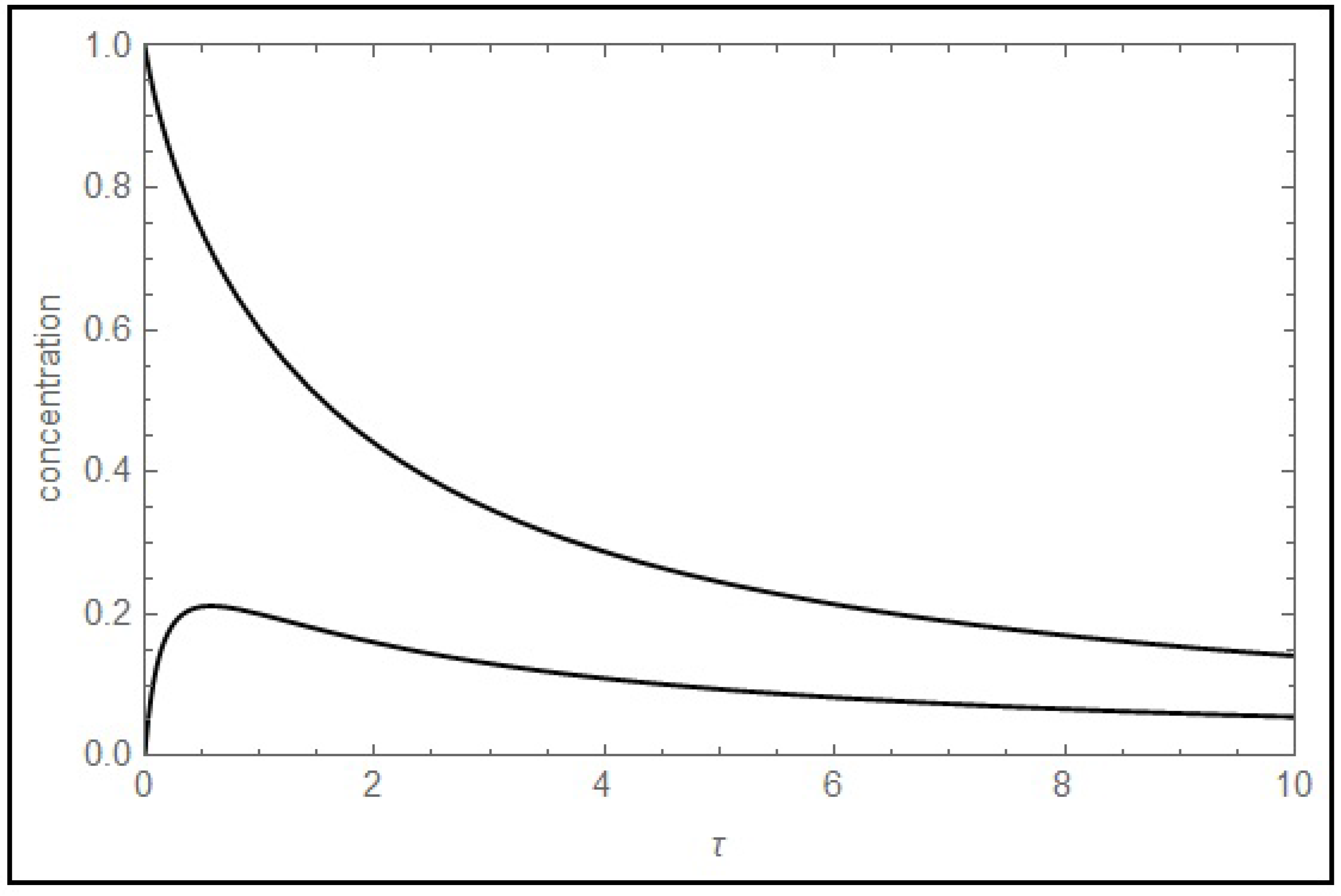
Figure 2. Impossibility of the intersection of ${\text{C}}_{{\text{A}}_{\text{A}}}$ (upper curve) and ${\text{C}}_{{\text{A}}_{\text{B}}}$ (lower curve) illustrated for the case (k₁⁺, k₁⁻, k₂) = (1, 2, 3 s⁻¹).

Figure 2. Impossibility of the intersection of ${\text{C}}_{{\text{A}}_{\text{A}}}$ (upper curve) and ${\text{C}}_{{\text{A}}_{\text{B}}}$ (lower curve) illustrated for the case (k₁⁺, k₁⁻, k₂) = (1, 2, 3 s⁻¹).

We observe maxima of concentration and rate curves only in three cases: ${\text{C}}_{{\text{A}}_{\text{B}}}$, ${\text{C}}_{{\text{B}}_{\text{A}}}$ and ${\text{R}}_{{\text{C}}_{\text{A}}}$. (see Table 2). All the maxima occur at the same space time. The maximum of the rate of formation ${\text{R}}_{{\text{C}}_{\text{A}}}$ exists, as the rate of formation of C is proportional to the concentration profile of B, i.e., ${\text{r}}_{\text{C}}\left(\text{τ}\right)={\text{k}}_2{\text{C}}_{\text{B}}\left(\text{τ}\right)$, see (2).

Table 2. Space time and values of the possible maxima.

Event	Space Time	Value
$max\left(C_{A_B}\right)$	$\frac{1}{\sqrt{k_1^{+}{k}_2}}$	$max\left(C_{A_B}\right)=\frac{k_1^{-}}{k_1^{-}+{\left(\sqrt{k_1^{+}}+\sqrt{k_2}\right)}^2}$
$max\left(C_{B_A}\right)$		$max\left(C_{B_A}\right)=\frac{k_1^{+}}{k_1^{-}+{\left(\sqrt{k_1^{+}}+\sqrt{k_2}\right)}^2}$
$max\left(R_{C_A}\right)$		$max\left(R_{C_A}\right)=\frac{k_1^{+}{k}_2}{k_1^{-}+{\left(\sqrt{k_1^{+}}+\sqrt{k_2}\right)}^2}$

Table 2. Space time and values of the possible maxima.

Event	Space Time	Value
$max\left(C_{A_B}\right)$	$\frac{1}{\sqrt{k_1^{+}{k}_2}}$	$max\left(C_{A_B}\right)=\frac{k_1^{-}}{k_1^{-}+{\left(\sqrt{k_1^{+}}+\sqrt{k_2}\right)}^2}$
$max\left(C_{B_A}\right)$		$max\left(C_{B_A}\right)=\frac{k_1^{+}}{k_1^{-}+{\left(\sqrt{k_1^{+}}+\sqrt{k_2}\right)}^2}$
$max\left(R_{C_A}\right)$		$max\left(R_{C_A}\right)=\frac{k_1^{+}{k}_2}{k_1^{-}+{\left(\sqrt{k_1^{+}}+\sqrt{k_2}\right)}^2}$

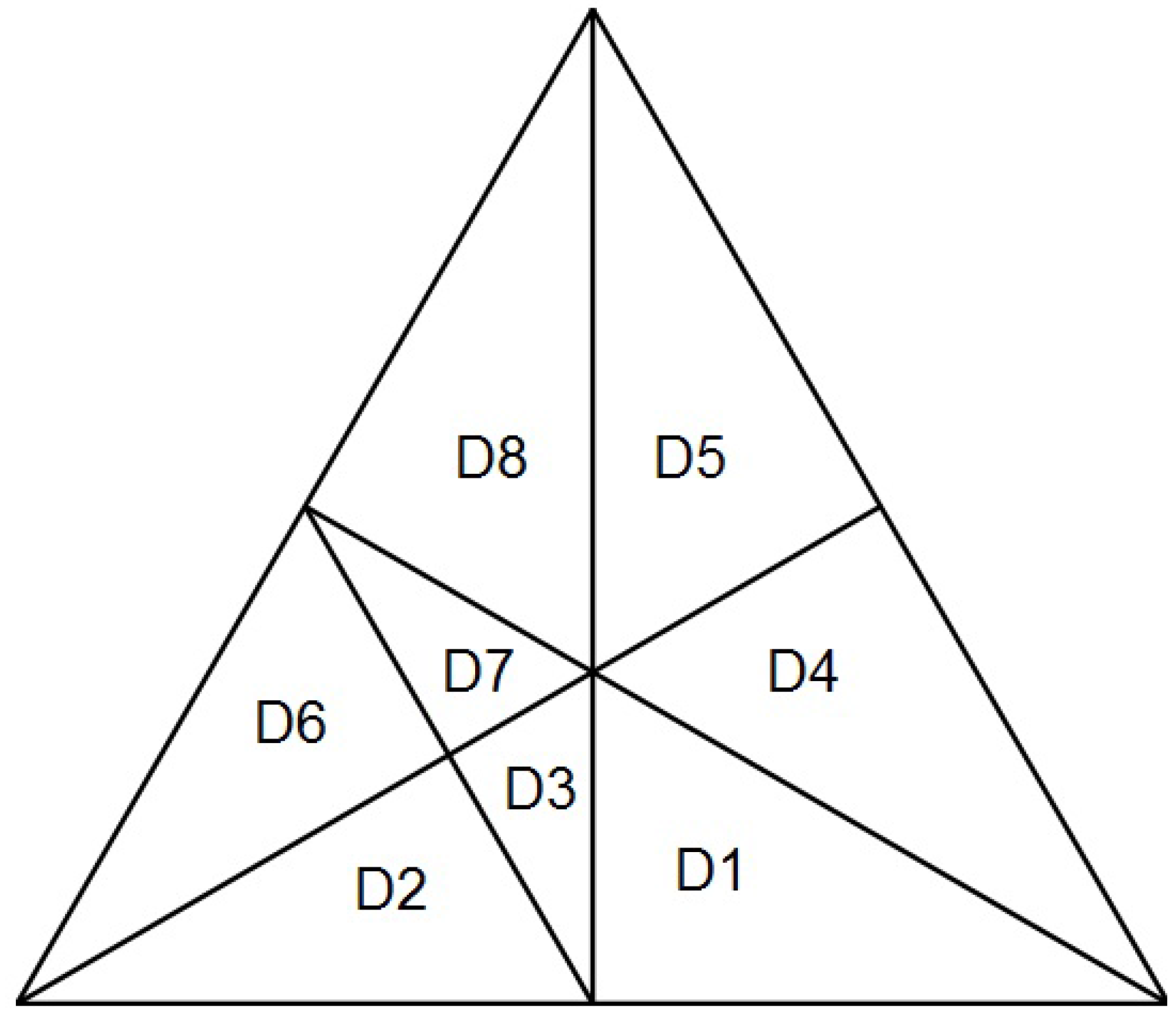
Analyzing the inequalities involving the kinetic constants of the conditional cases depicted in Table 1, we can differentiate eight domains of existence, shown in Table 3. The existence of the events is associated with the validity of the conditional expressions in the first column. The rest of the columns describe the possible combinations of validity of the conditional expressions, being eight in total. The domains are plotted in Figure 3. The equilateral triangles represent triples (k₁⁺, k₁⁻, k₂) in barycentric coordinates; the vertex at 12 o’clock represents pure k₂, i.e., (0, 0, 1); the vertex at 4 o’clock, pure k₁⁻, i.e., (0, 1, 0), and the vertex at 8 o’clock represents pure k₁⁺, i.e., (1, 0, 0). For a given point, the values (k₁⁺, k₁⁻, k₂) are obtained by measuring the shortest distance between the point and the left side, right side, and the base of the triangle, respectively.

Figure 3. Barycentric plot showing the eight possible domains listed in Table 3.

Figure 3. Barycentric plot showing the eight possible domains listed in Table 3.

Table 3. Domains for the existence of intersections between concentration time dependences.

	D1	D2	D3	D4	D5	D6	D7	D8
$k_1^{+}>k_1^{-}+k_2; C_{A_A}=C_{B_A}$	No	Yes	No	No	No	Yes	No	No
$k_1^{+}>k_2$; $C_{B_A}=C_{C_B}; R_{B_A}=R_{C_B}$	Yes	Yes	Yes	No	No	Yes	Yes	No
$k_1^{-}>k_1^{+}$; $C_{A_B}=C_{B_B}$	Yes	No	No	Yes	Yes	No	No	No
$k_1^{-}>k_2$; $C_{A_B}=C_{C_B}; R_{A_B}=R_{C_B}$	Yes	Yes	Yes	Yes	No	No	No	No

Table 3. Domains for the existence of intersections between concentration time dependences.

	D1	D2	D3	D4	D5	D6	D7	D8
$k_1^{+}>k_1^{-}+k_2; C_{A_A}=C_{B_A}$	No	Yes	No	No	No	Yes	No	No
$k_1^{+}>k_2$; $C_{B_A}=C_{C_B}; R_{B_A}=R_{C_B}$	Yes	Yes	Yes	No	No	Yes	Yes	No
$k_1^{-}>k_1^{+}$; $C_{A_B}=C_{B_B}$	Yes	No	No	Yes	Yes	No	No	No
$k_1^{-}>k_2$; $C_{A_B}=C_{C_B}; R_{A_B}=R_{C_B}$	Yes	Yes	Yes	Yes	No	No	No	No

3. Direct Application of the Intersection Characteristics (Times and Concentration Values)

The expressions for the value and space time of the events shown in Table 1 and Table 2 are useful to calculate directly the kinetic constants. For example, the value of k₂ can be found as the inverse of the space time at the intersection of the events ${\text{C}}_{{\text{B}}_{\text{A}}}$ = ${\text{C}}_{{\text{C}}_{\text{A}}}$, ${\text{C}}_{{\text{B}}_{\text{B}}}$ = ${\text{C}}_{{\text{C}}_{\text{B}}}$, and ${\text{R}}_{{\text{B}}_{\text{A}}}$ = ${\text{R}}_{{\text{C}}_{\text{A}}}$ (see Table 1). Knowing then the space time at the intersection of the events ${\text{C}}_{{\text{C}}_{\text{A}}}$ = ${\text{C}}_{{\text{A}}_{\text{B}}}$ or ${\text{R}}_{{\text{C}}_{\text{A}}}$ = ${\text{R}}_{{\text{A}}_{\text{B}}},$ k₁⁻ / (k₁⁺k₂), see Table 1, we can extract the inverse equilibrium constant, K_eq = k₁⁻/k₁⁺. From the inverse of the space time at the intersection ${\text{C}}_{{\text{A}}_{\text{B}}}$ = ${\text{C}}_{{\text{B}}_{\text{B}}}$, 1/(k₁⁻ − k₁⁺), we can obtain the difference between these two kinetic constant of the reversible reaction. As a result, we are able to determine all parameters from three independent values of intersection space times. The chosen intersections can be considered as independent events, and other events can be considered as dependent ones and their characteristics can be calculated using only three determined kinetic parameters. Certainly, we can choose different sets of independent events, all listed in Table 1 and Table 2. The most convenient choice can be based on simplicity of the analytical expressions. It is interesting to use the expression for the space time of the maxima, τ_max = (k₁⁺k₂)^−1/2 given in Table 2, as, for example, ${\text{τ}}_{\left({\text{C}}_{{\text{C}}_{\text{A}}}={\text{ C}}_{{\text{B}}_{\text{B}}}\right)}{{\text{τ}}_{max}}^2=$ k₁⁻. Parallel comparison of the kinetic constants obtained from different events is an elegant test to validate the kinetic model.

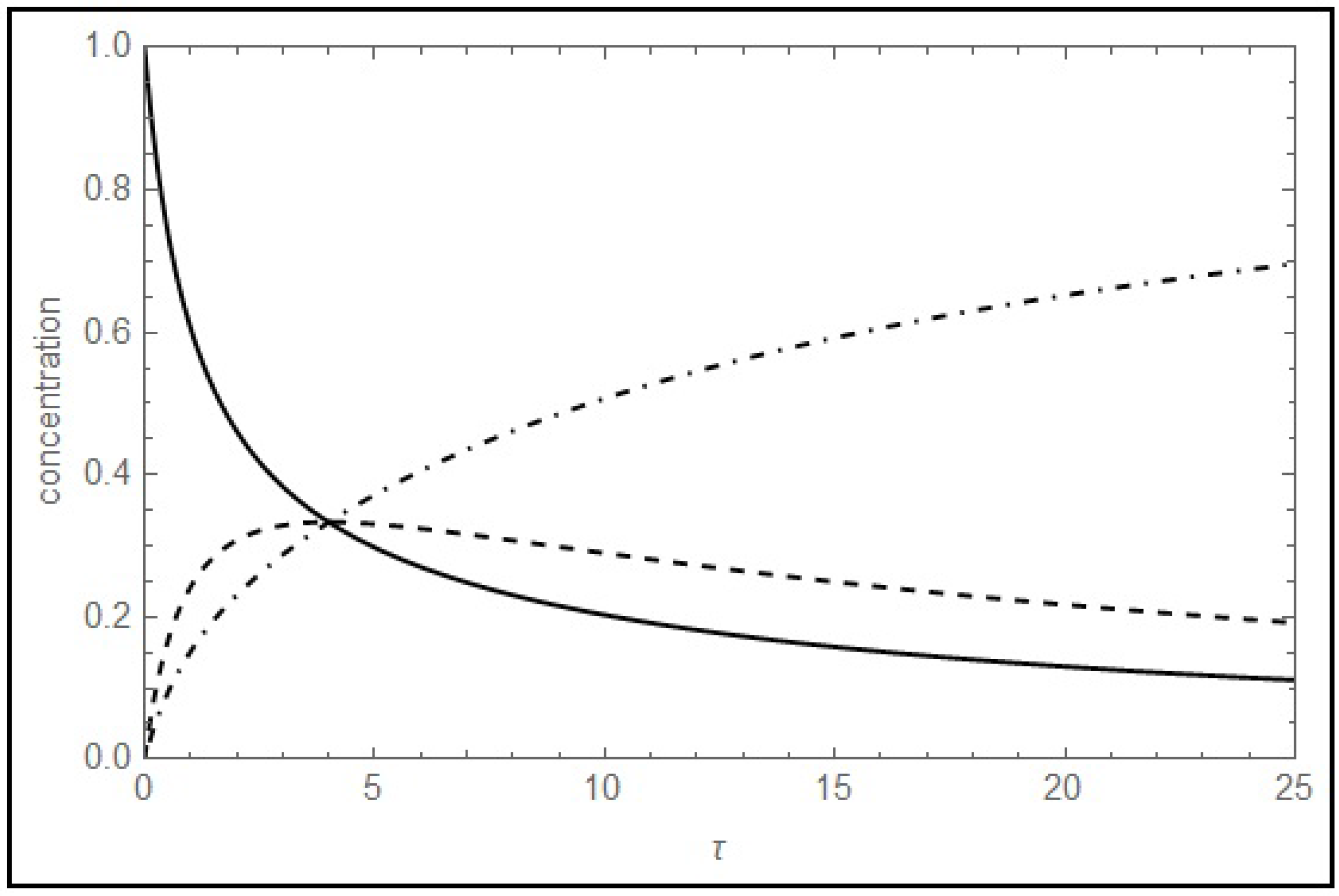
An interesting case is the invariant space time of the intersection between the concentration profiles of B and C, C_B(τ) and C_C(τ), respectively. As mentioned, assuming the initial concentration of C, C_C(0) = 0, the space time of intersection is 1/k₂. This result is general, and it doesn’t depend on the origin of B, i.e., the space time of the intersection doesn’t vary if we start from pure B, or if B is produced from pure A. Furthermore, we can expand this result to a system consisting on a cascade of reactions, ending with an irreversible one: the space time of the intersection for the two chemical species involved in the irreversible reaction corresponds to the inverse of its kinetic coefficient. This result is restricted if the two trajectories for these chemical species depart from the same reagent, whichever it is. This is an important result and a fingerprint of the described kinetic model in a CSTR. A special case is obtained if k₁⁺ = k₂; if so, the space time corresponding to maximum of the curves listed in Table 2 coincides with 1/k₁⁺ = 1/k₂, and a triple intersection is observed: in Figure 4 is shown an illustration of this triple intersection. Further discussion of the existence of triple intersections will be given in the next section.

Figure 4. Triple intersection between ${\text{C}}_{{\text{A}}_{\text{B}}}$ (dashed curve), ${\text{C}}_{{\text{B}}_{\text{B}}}$ (solid curve) and ${\text{C}}_{{\text{C}}_{\text{B}}}$ (dot-dashed curve) at τ = 1/k₁⁺, for the case (k₁⁺, k₁⁻, k₂) = (k₁⁺, 2k₁⁺, k₁⁺). k₁⁺ = 0.25 s⁻¹.

Figure 4. Triple intersection between ${\text{C}}_{{\text{A}}_{\text{B}}}$ (dashed curve), ${\text{C}}_{{\text{B}}_{\text{B}}}$ (solid curve) and ${\text{C}}_{{\text{C}}_{\text{B}}}$ (dot-dashed curve) at τ = 1/k₁⁺, for the case (k₁⁺, k₁⁻, k₂) = (k₁⁺, 2k₁⁺, k₁⁺). k₁⁺ = 0.25 s⁻¹.

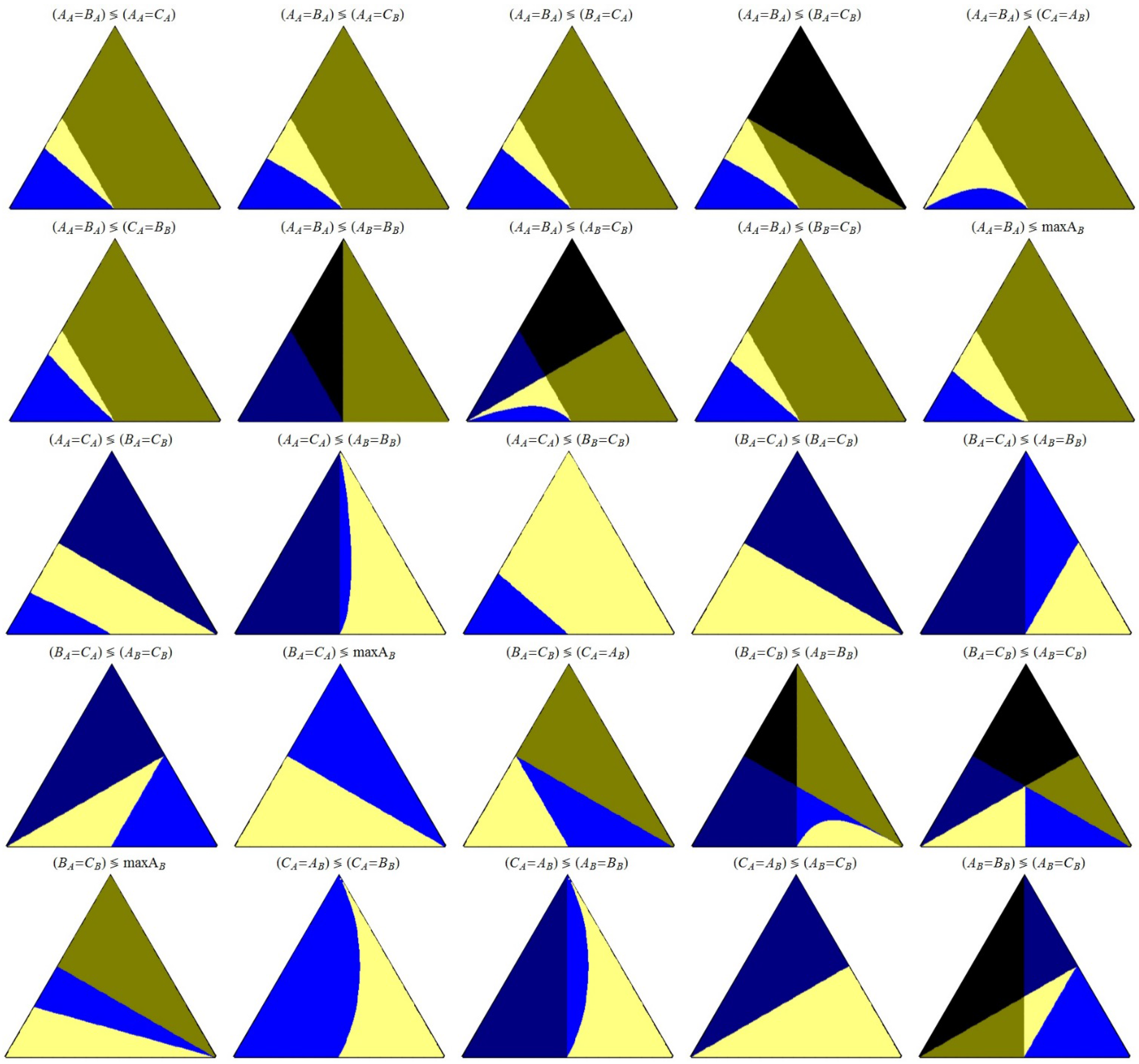
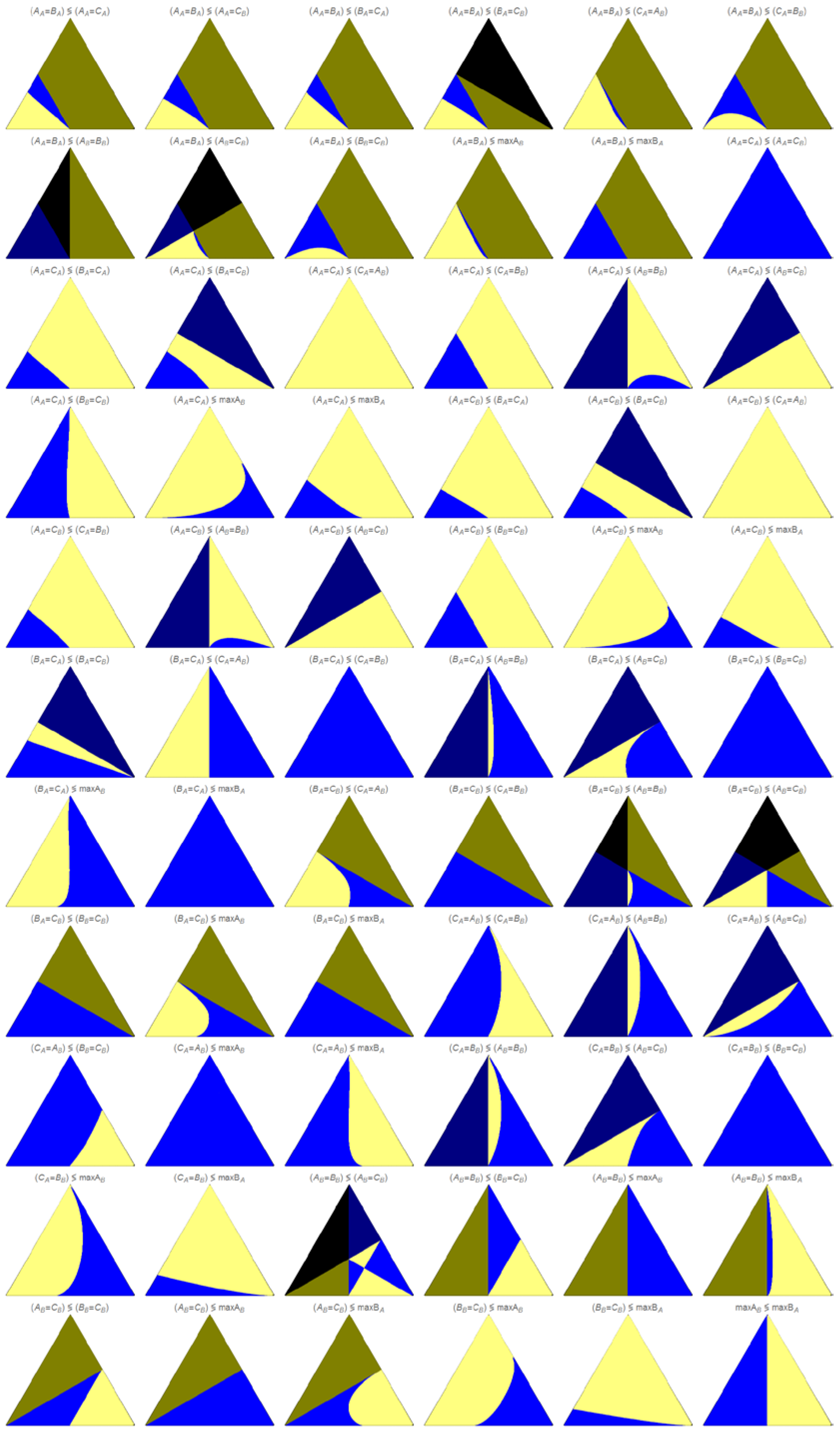
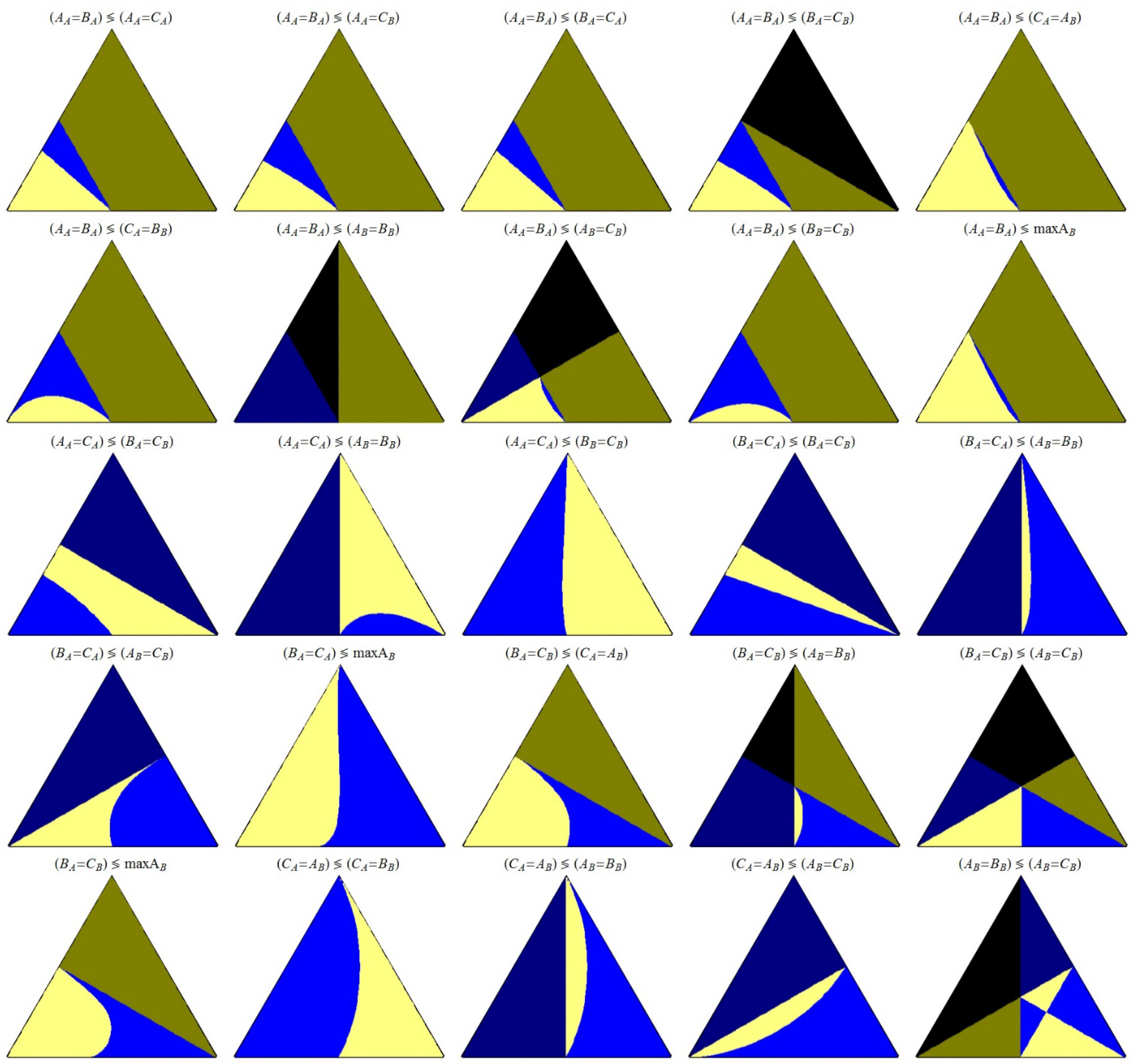
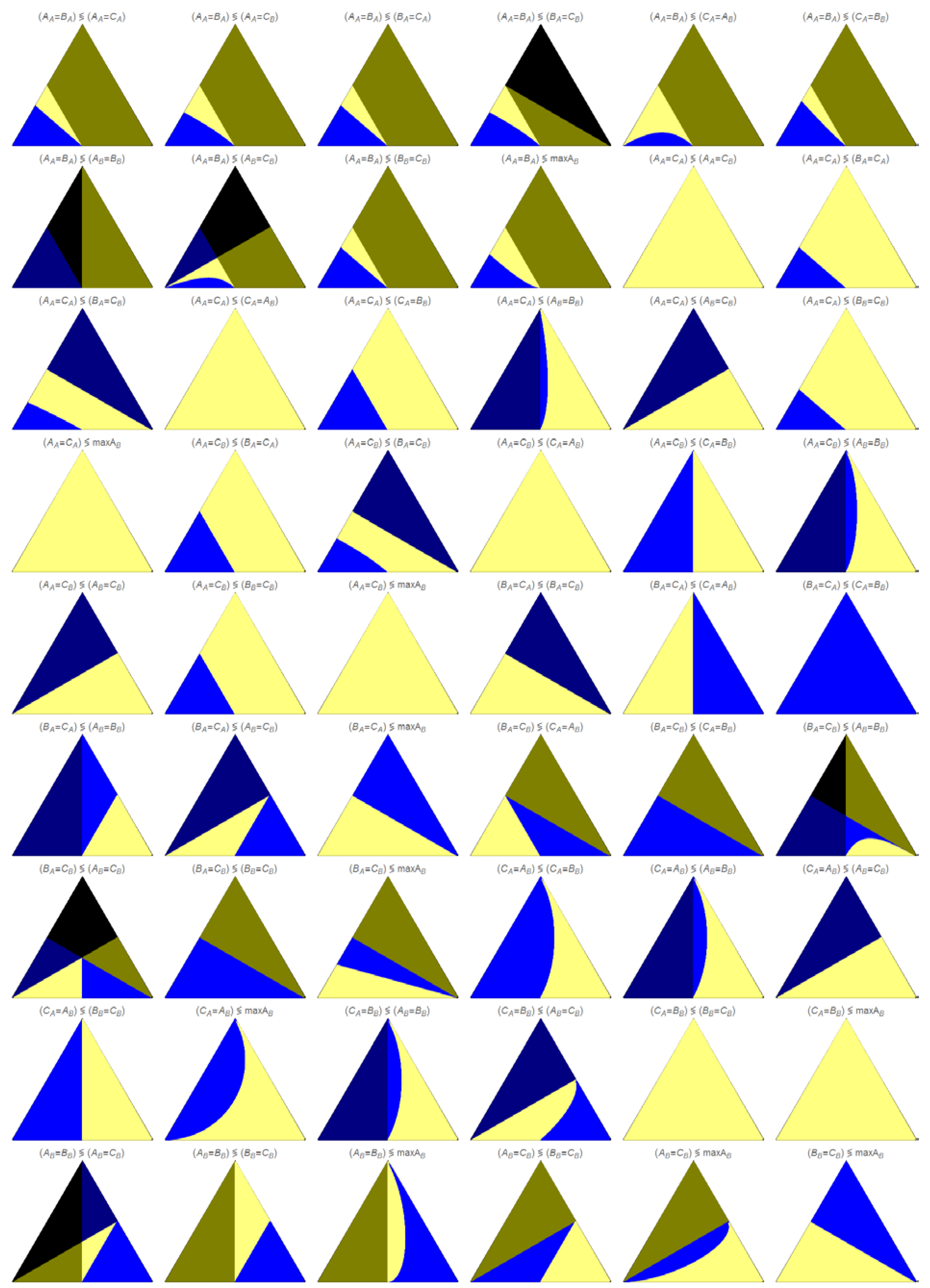
4. Ordering Domains and Coincidences

The relationship between each pair of events are shown in Figure 5, Figure 6 and Figure 7. The values (space time, concentration, or rate, depending on the figure) at each region are ranked depending on the color legend, as follows: if both events exists and the corresponding left value is smaller, the region is colored in light blue, whereas if the right value is smaller, the color is light yellow. The regions where only exists the left side are colored in dark blue, and the regions where exists exclusively the right side are colored in dark yellow. Black means that neither the left nor the right side exists. In the appendix is shown the analysis of two examples in Figure 6.

Let’s focus our attention in Figure 5, where is shown the comparison between the corresponding space time values at the intersection of several pairs of events. In the plots we have two colors that indicate a partial restriction (dark yellow and dark blue), and one color indicating a total restriction (black, so both the left and the right event are not observed). In this case, if an event is restricted it means that the value of the space time when the event takes place is negative. The limits of the regions between these three colors correspond to the points (k₁⁺, k₁⁻, k₂) where at least one value of space time (left or right) is zero, as follows: the limit dark yellow–black corresponds to space time of the right side event equal to zero; the limit dark blue–black corresponds to a space time of zero for the left side event.

Figure 5. Ordering of the space time values for the indicated pair of events.

Figure 5. Ordering of the space time values for the indicated pair of events.

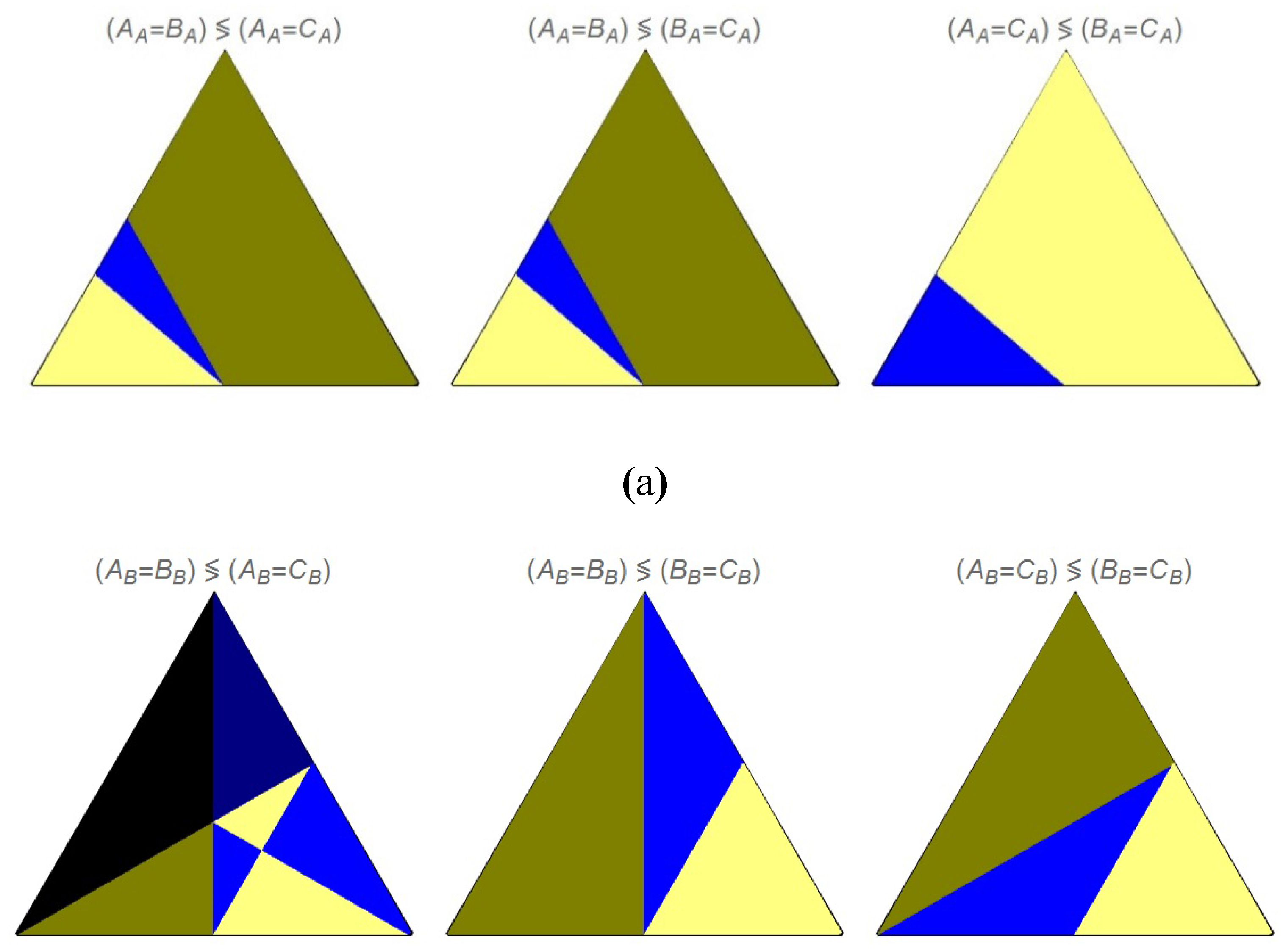
No intersection occurs between regions colored in dark blue and dark yellow, excepting single point intersections between regions in black, dark blue and dark yellow, as seen in Figure 5, (A_A=B_A) $\lessgtr$ (A_B=C_B), (B_A=C_B) $\lessgtr$ (A_B=B_B), (B_A=C_B) $\lessgtr$ (A_B=C_B) and (A_B=B_B $\lessgtr$ (A_B=C_B). At these single point intersections, both the right and the left side events have a value of space time equal to zero. These four combinations of intersections are the only ones that show all the five colors, and all possible cases arise, depending on the values of the parameters.

We should stress out that the regions of the triangular plots shown in Figure 5 that are colored in black, dark blue or dark yellow, are replicated exactly, and with the same colors, in Figure 6, where is shown the comparison between the concentration values of the same pair of events, because the event happens at a negative value of space time, and so is restricted, and not observed. As it is possible to obtain positive values of concentration at negatives values of space time, we are no able to interpret the limits between the colors black–dark blue and black–dark yellow as points (k₁⁺, k₁⁻, k₂) of zero concentration for the left or right event, respectively. One of the figures in Figure 5, A_A=C_A $\lessgtr$ A_B=B_B, which contains only these three colors, is exactly the same in Figure 6; this is the only case where a figure contains only these “restrictive” colors.

Figure 6. Ordering of the concentration values for the indicated pair of events.

Figure 6. Ordering of the concentration values for the indicated pair of events.

The regions colored in light blue or light yellow indicate the existence of the two compared events. For the points (k₁⁺, k₁⁻, k₂) where the value of the left side event is larger than the value of the right side event, the point is colored in light yellow, or in light blue otherwise. The points limiting the regions colored in light yellow and light blue corresponds to points of equal value of the two compared events. When comparing these regions in the triangular plots shown in Figure 5 and Figure 6, we can observe that the total region occupied by these colors remains unchanged, for the same comparison of events, but the relative distribution of both light blue and light yellow colored regions can change. For some of the triangular plots, these two colors occupy all the equilateral triangle: (A_A=C_A) $\lessgtr$ (B_B=C_B), (B_A=C_A) $\lessgtr$ (B_A=C_B), (B_A=C_A) $\lessgtr$ maxA_B and (C_A=A_B) $\lessgtr$ (C_A=B_B), in both Figure 5 and Figure 6. This last case, (C_A=A_B) $\lessgtr$ (C_A=B_B), and also (B_A=C_B) $\lessgtr$ (A_B=C_B), are the only cases where both light blue and light yellow regions remain unchanged in Figure 5 and Figure 6.

Figure 7. Ordering of the rate values for the indicated pair of events.

Figure 7. Ordering of the rate values for the indicated pair of events.

Figure 8. Ordering of the concentration values for the indicated pair of events, (a) departing from pure A, and (b) departing from pure B.

Figure 8. Ordering of the concentration values for the indicated pair of events, (a) departing from pure A, and (b) departing from pure B.

In Figure 8 are shown the comparison of the concentration values at the intersections of two series of concentration profiles: in Figure 8a, (A_A=B_A) $\lessgtr$ (A_A=C_A), (A_A=B_A) $\lessgtr$ (B_A=C_A) and (A_A=C_A) $\lessgtr$ (B_A=C_A), all departing from A, and in Figure 8b, the same set of comparisons but departing from B. In the first series of triangular plots, in Figure 8a, we can observe that the three plots share an unique curve, k₁⁺ = k₁⁻ + 2k₂, delimiting two regions colored in light blue and light yellow: at these values of the kinetic constants, there is a triple intersection between the concentration profiles obtained starting from A: A_A, B_A and C_A. On the other hand, in the Figure 8b, the limiting curve between the light blue and light yellow colored regions, repeated in the corresponding three plots, is k₁⁻ = k₁⁺ + k₂; a triple intersection occur at those values of the kinetic constants that satisfy this equation between the concentration profiles departing from B: A_B, B_B and C_B. Besides, in this case, if k₁⁺ = k₂, the intersection occurs at the maximum of A_B: this special point (k₁⁺, k₁⁻, k₂) = (0.25, 0.50, 0.25 s⁻¹), is observed in Figure 8b, for the case (A_B=B_B) $\lessgtr$ (A_B=C_B)_, in the crossing point of the curves k₁⁻ = k₁⁺ + k₂ and k₁⁺ = k₂, and illustrated in the plots shown in Figure 4.

An interesting remark are the values of the intersections of some of the curves shown in Figure 5 and Figure 6, at the sides of the equilateral triangles. These intersections points were studied previously for the case where k₁⁻ = 0, i.e., A→B→C, by Yablonsky et. al. [3]; they defined some special points: the Euler point, k₁⁺ = k₂; the Acme point, k₁⁺ = 2k₂, and the Golden point, k₁⁺ = ϕ·k₂, where ϕ is the golden ratio, ϕ = ($\sqrt{5}$ + 1) / 2 = 1.618034…. The Euler point, at the middle of the left side of the triangular plots, appears in several of the plots shown in Figure 5 and Figure 6. The Acme point can be observed, for instance, in the plots for (A_A=B_A) $\lessgtr$ (A_A=C_A) in both figures, in (A_A=C_A) $\lessgtr$ (B_B=C_B) in Figure 5, and in (B_A=C_A) $\lessgtr$ (A_B=B_B) in Figure 6. The Golden point can be observed in some intersections at the base side of the triangular points (k₂ = 0) in Figure 6: in (B_A=C_A) $\lessgtr$ maxA_B and (B_A=C_B) $\lessgtr$ maxA_B. Simple functions of the Golden point can be observed in some triangular plots at k₁⁻ = 0, in Figure 5: in (A_A=B_A) $\lessgtr$ (A_A=C_B), (A_A=B_A) $\lessgtr$ (B_A=C_B), (A_A=B_A) $\lessgtr$ maxA_B and (B_A=C_B) $\lessgtr$ maxA_B, intersections at the left side of the triangular plots occur at k₁⁺ = (ϕ + 1)k₂. The reader is referred to Figure A2 and Figure A3 in the appendix to find the full spectrum of plots for comparisons in space time and concentration.

5. Conclusions

For steady-state kinetic models of CSTRs, there were found new patterns of kinetic behavior, similar to previous results for non-steady kinetic models of BR and TAP reactor. It was demonstrated using two-step mechanism A↔B→C as an example. There were obtained simple relationships between characteristics of these patterns, i.e., space times of kinetic dependences intersections and maxima, values of concentrations and reaction rates as well. It was shown that these relationships are useful for efficient determining the kinetic parameters. For the pair of species involved into the irreversible reaction (B and C), the space time of their corresponding concentration dependence intersection is invariant and does not depend on the initial conditions of the system. Map of patterns were presented for visualization of their combinations and ranking in space time, and values of concentration and rates. These maps can be useful for predicting kinetic behavior and for mechanism discrimination. In the future, these studies will be continued for more general cases, taking advantage of the simplicity of the algebraic CSTR models in comparison with differential models of BR and TAP reactors.