1. Introduction
Logistics management plays an important role in reducing costs and improving the competitiveness of enterprise. The logistics companies have to make strategic and operational decisions to schedule the business processes more efficiently. Many companies use the method of optimizing vehicle routes so as to reduce costs and to improve logistic service quality effectively. Among them, the vehicle routing problem (VRP) draws great interest, which presents promising performance in chain management and many other areas. The VRP can be defined as determining an optimal set of routes for vehicles, which would save time and cost, so as to effectively strengthen the logistic companies’ competitiveness. One variants of VRP is the vehicle routing problem with time windows (VRPTW). VRPTW imposes the appropriate time window and time constraints to each task node (including dispatch node and receiving node) on the basic VRP. In this way, VRPTW is able to improve service quality. VRPTW has a wide range of applications, such as distribution requirements planning [
1,
2], material handling systems [
3], bank deliveries [
4], postal deliveries [
5], school bus routing [
6] and so on. Actually, VRPTW has been a research field of great interest, and many different solving algorithms have been proposed.
Despite its great potential in solving the vehicle routing problem, VRPTW is still a difficulty, since it belongs to NP-hard problems. Many researchers put forward a variety of accurate methods to solve the problem, such as Multi-Objective Programming, Linear Programming and Integer Programming. These polynomial methods with constraints can perform effectively and get the optimal solution in the small-scale VRP. However, with the increase of the problem scale, it needs much more time to match the explosive growth. Therefore, much effort has been done on the heuristic intelligent algorithm to solve VRPTW. The heuristic algorithm is simple to implement and does not present an obvious time increase with the problem scale increasing. The main problem is that the iteration speed is slow in the early stage, and it is easy to fall into local optimal solutions. In a word, both the accurate solution and heuristic solution have weakness on solving VRPTW.
Nowadays, the problem scale of real-world VRPTW increases rapidly. The accurate algorithms need too much time to model and search for a proper solution, while single heuristic algorithms often fall into local optimal solutions and need a large number of iteration times. This paper gives a new insight into VRPTW and proposes an effective method by combining different VRPTW solutions. Particle swarm optimization (PSO) is a promising method, since its iteration speed is fast. However, it often falls into local optimal solution. The chaos optimization algorithm (COA) and the Gaussian strategy can upgrade solution diversity and avoid falling into the local optimal. The insertion heuristic algorithm can construct the initial solution quickly and upgrade iteration speed. So, this paper combines these algorithms and proposes a hybrid chaos-particle swarm optimization algorithm (HPSO) for VRPTW. The contributions of this paper are as follows:
- (1)
A PSO based on COA is proposed, so as to avoid the problem that the number of the feasible solution particles is too small in the early state and the speed of the convergence is low. When the feasible solution particle first appears, COA is able to re-initialize the particle swarm, which can increase the number of the feasible solution particles and accelerate the convergence.
- (2)
The insertion heuristic algorithm is introduced into our method to construct the route of VRPTW in the decoding process, which is much easier and more effective than conventional methods.
- (3)
COA and Gaussian strategy are used to judge the premature convergence and to improve the particle swarm when the solving process falls into local optimal solutions.
The remainder of this paper is organized as follows.
Section 2 introduces the related work;
Section 3 describes the VRPTW model;
Section 4 details the proposed HPSO;
Section 5 presents various experiments to compare HPSO with other state-of-the-art methods on solving VRPTW. Finally is a summary of the paper and future outlooks.
2. Related Work
Many researchers used different heuristic algorithms for VRPTW. Instead of obtaining the optimal solution of VRPTW, like the accurate algorithms, heuristic algorithms can quickly get the approximate optimal solution. When the problem scale of VRPTW is large, the advantage of the heuristic algorithm is more obvious. Thus, early studies are based on single heuristics and metaheuristic, such as local search [
7], minimum K-trees [
8], adaptive memory [
9], simulated annealing (SA) [
10], tabu search (TS) [
11,
12], genetic algorithm (GA) [
13] and ant colony optimization (ACO) [
14]. When the problem scale of VRPTW is small, these methods mentioned above can get an optimal result with limited time. However, when the problem scale of VRPTW increases, they will easily fall into the local optimal, and the iteration time cost will increase explosively. So, nowadays, many researchers focus on combing two or three heuristics and metaheuristic methods to solve VRPTW.
- (1)
A typical hybrid method is TS combined with other algorithms [
15,
16,
17]. Tabu search keeps a list of forbidden transformations to transfer the solution step that deteriorates the objective function value; while a hybrid algorithm based on TS and variable neighborhood descent uses a sweep method to obtain an initial solution [
18].
- (2)
Local search combined with other algorithms was also proposed to solve VRPTW. Bianchessi et al. citeR19 proposed a local search heuristic method based on TS using a variable neighborhood structure, in which the node-exchange-based and arc-exchange-based movements are combined. Gendreau et al. [
20] proposed a hybrid neighborhood search heuristic to optimize the planned route of vehicle in a context, where new requests with a pick-up and a delivery location would occur in real-time. Zachariadis et al. [
21] proposed a hybrid local search approach based on TS, which can efficiently examine the rich solution neighborhood by statically encoding tentative moves into the special data of a diversification component, which is based on the aspiration criteria of TS. Hong [
22] proposed a hybrid and improved the large neighborhood search (I-LNS) algorithm to solve the VRPTW. Utilizing the remove-reinsert process of the LNS, the latest request nodes are regarded as a part of the removed nodes; these nodes can be inserted into the original or current solution in good time in the reinsertion process; meanwhile, its computing speed is high and effective, for it does not need to resolve the primal problem each time.
- (3)
SA combined with other algorithms was used to solve VRPTW. Tavakkoli-Moghaddam et al. [
23] proposed a liner-integer model based on SA, which constructs VRPTW with the independent route length in order to minimize the heterogeneous fleet cost and the capacity utilization. TTavakkoli-Moghaddam et al. [
24] also proposed a new mathematical model based on SA to find the short routes with the minimum fleet travel cost, the minimum travel distances and the maximum sale.
- (4)
ACO combined with other algorithms provided another way to solve VRPTW [
25,
26,
27]. The weakness of ACO for VRPTW is that ants tend to create infeasible solutions with non-routed clients. Most implementations of ACO combined with other algorithms return feasibility to the solutions by applying a simple
ad hoc post-insertion procedure, and when the post-insertion fails to route all the clients, the partial solution is discarded.
- (5)
GA can also be combined with other algorithms to solve VRPTW [
28,
29]. GA mimics the evolution process in solving problems. The basic operation is the mating of two tours in order to form a new tour. Moreover, GA combined with other algorithms uses algorithmic anagoges to mutation and selection. The weakness of GA for VRPTW is the encoding of the chromosome. With the problem scale increase, the difficultly of encoding the chromosome increases.
From the above brief review of different hybrid methods, it is concluded that many attempts have been made to solve VRPTW by combining different approaches. Two main properties of all the above methods in the literature can be summarized as follows: (1) Firstly, use a heuristic method to obtain a feasible initial solution; (2) Then, hybridize the metaheuristic method with another heuristic method to improve the solution during the iteration process. Particle swarm optimization (PSO) is a recent and promising evolution metaheuristic and has been successfully applied to solve VRPTW. Many researchers conduct research on solving VRPTW by combining PSO with other heuristic methods. Chen et al. [
30] proposed a discrete PSO algorithm combined with SA heuristics. He got the high precision vehicle routes for some vehicle routing problems with less than 134 customers. However, the algorithm would cost a lot of computing time. In the worst case, it would cost more than half an hour to get the solution. Kachitvichyanukul [
31] proposed two new PSO algorithms (SR-1 and SR-2) for encoding and decoding particles into vehicle routes. By comparing SR-1 with SR-2, he got the conclusion that SR-2 is better than SR-1. Zhao et al. [
32] proposed a new encoding method based on PSO. They conducted a 2L-dimensional position vector of particles. Among them, L represented the number of service customers. Then, 2L-dimensional space corresponding to each particle was divided into two L-dimensional vectors: one vector meant the vehicle number for each customer, and the other vector represented the service order for each customer in the vehicle route. As to the particle decoding process, Zhang et al. [
33] proposed a simulated annealing algorithm to construct the vehicle route. Firstly, they used PSO to solve the sub-problem of task assignment. Then, they used the simulated annealing algorithm to solve the sub-problem of route optimization. In order to get the infeasible solutions for particle swarm, Wu et al. [
34] put forward a local neighborhood mechanism to increase the diversity of the particles and avoid falling into the local optimal state. Gong et al. [
35] proposed a set-based PSO to solve the discrete combinatorial optimization VRPTW and achieved better effectiveness and efficiency. All the above PSO based methods can get a satisfied solution, but when the problem scale increases, it will cause problems, such as the speed of the iteration becoming slow in the early stage and it is easy to fall into local optimal solutions.
Aiming at alleviating the above problems, this paper puts forward a new hybrid algorithm, HPSO. It uses the advantage of the COA and Gaussian strategy to upgrade basic PSO solution diversity to avoid falling into the local optimal. COA is also beneficial for accelerating the iteration in the early stage. This paper also proposes an insertion heuristic algorithm to construct the initial solution and upgrade the iteration speed, as basic PSO is difficult for constructing the initial solution.
3. VRPTW Model Formulation
VRPTW as an extension of the basic vehicle routing problem is generally described as: one yard has K cars. The deadweight of each car is . There are L customers who need service. Customer i demands the goods . It assumes that the time of service for customer i is , and the start time of service is a certain range of time, means the earliest start time and means the latest start time ). If the vehicle arrives earlier than , the vehicle need to wait until . If the vehicle arrives later than , customer i needs to be delayed. At last, it finds the vehicle route that costs least. The mathematical model is described as follows:
The yard number is defined as 0, the customers are defined as , and and so point, , can represent the yard and the customers.
The symbols in the model are defined as follows:
is the transportation costs of i to j, which refer to the costs of distance and time.enumerate
is the time of vehicle arrival for customer j.
is the cost per unit of time for the vehicle to wait for the customer.
is the fine per unit of time for a later vehicle arrival.
is the cost of waiting when the vehicle arrives earlier than .
is the fine of vehicle arrival later than .
K is the number of all vehicles.
is the demand quantity of customer i.
is the capacity of vehicle k.
is service time.
is the travel time between customer i and customer j.
is the waiting time of a vehicle at customer i.
Based on the symbols, we can obtain the VRPTW mathematical model as Equation (1):
The constraints are defined as follows:
- (1)
On each route, the sum of each customer’s demand cannot exceed the capacity of the vehicle, which is defined as Equation (2):
- (2)
Each customer must get the delivery service, which is defined as Equations (3) and (4):
- (3)
The service for each customer can only be completed by a specific vehicle, which is defined as Equations (5) and (6):
- (4)
Variables in the range are defined as Equations (7) and (8):
- (5)
Time window constraints are defined as Equations (9) and (10):
The objective function of the mathematical model consists of three parts, including toll costs, waiting time costs and delay fine costs. The goal is to get the minimum value of the total costs. In addition, set the parameter and , we can get the model of the corresponding vehicle routing problem with hard time windows and the model with soft time windows. If is infinity, we can get the model of the vehicle routing problem with hard time windows. At the same time, the model also ensures that the vehicle route does not have the local sub-loop. Besides, the model set the fine costs when the vehicle arrives earlier or later. To get the least total costs, the solution has to avoid or minimize the fine costs.
4. HPSO
HPSO is based on PSO. To improve the quality of the particle in the early stage, we use the global optimal particle by COA to re-initialize the particle swarm. At last, we judge the premature convergence and use COA and Gaussian mutation to avoid falling into the local optimal state. Algorithm 1 is shown as follows:
| Algorithm 1 HPSO |
| Input: maximum number of iterations T |
| Output: the optimal solution |
- 1:
Randomly initialize the swarm particle encoding, then decode the particle and get the fitness value of the particle’ note . (Algorithm 2) - 2:
When getting the feasible particle solution, use the global optimal particle by COA to re-initialize the particle swarm and get the new particle swarm including n particles; note . Go to Step 3, otherwise go to Step 4. (Algorithm 3) - 3:
Judge the degree of the premature convergence: assume that the average optimal fitness value of the particle in history has not changed for N rounds; if , optimize the global optimal particle by COA; if and the probability of particle randomly generated is , convert the particle by Gaussian Mutation. , and are predetermined constants. - 4:
Update the speed and position of the particles: decode the particles and calculate the fitness value of particles; update the local best value, ; obtain the global best, . - 5:
If the current number of iterations , go to Step 6; otherwise, when , go to Step 2; or if the last, go to Step 3. - 6:
Stop updating particles; quit.
|
4.1. The Encoding and Decoding of the Particles
This paper proposes an encoding method. It assumes that there are
K vehicles, and
L customers. It constructs particles in
-dimensional space, in which each dimension is described by a real number. The front
L-dimensions are the total number of the customers, and the later
-dimensions are the position of the
K vehicles in the Descartes figure.
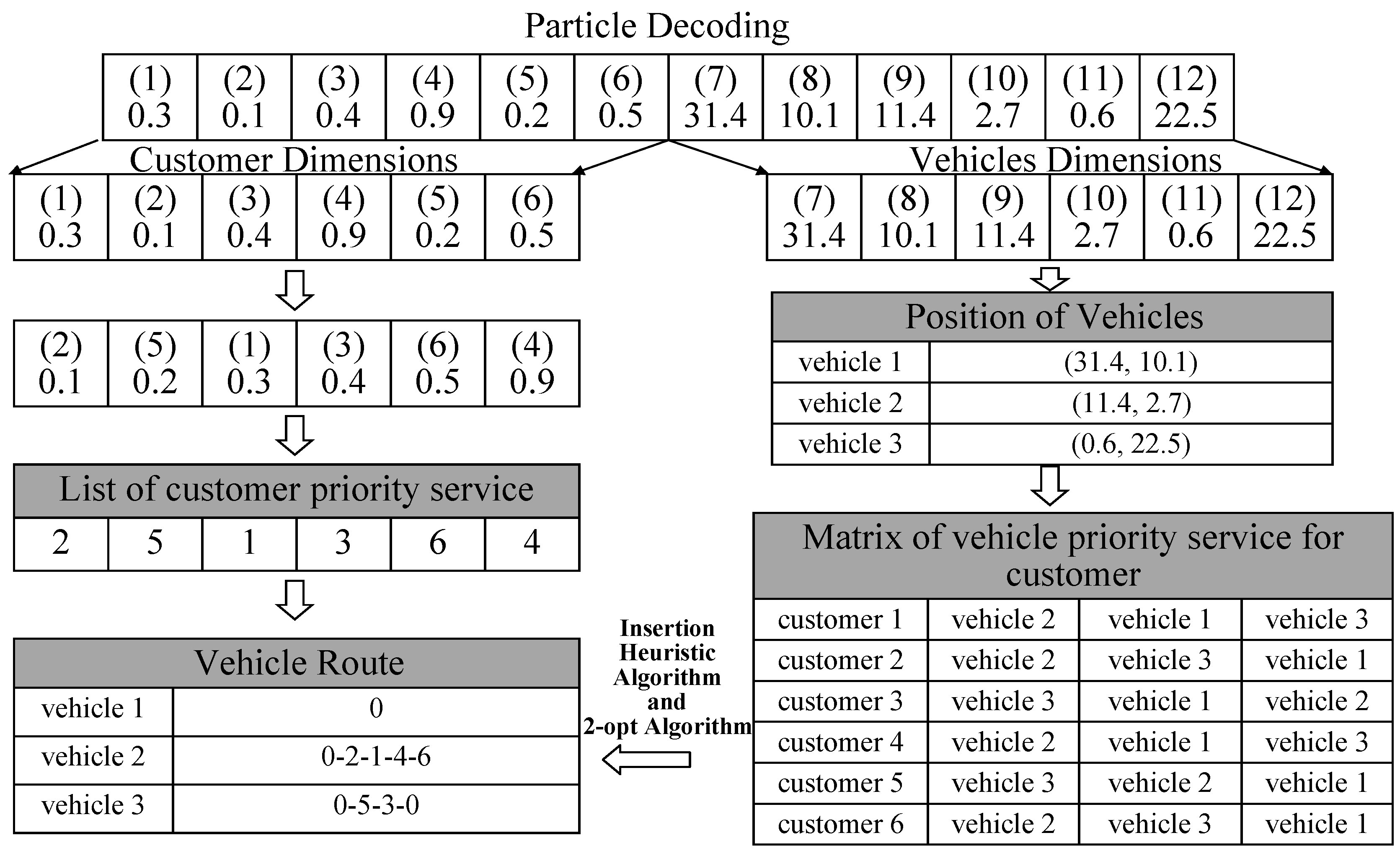
Figure 1.
Particle decoding and the set of vehicle routes.
Figure 1.
Particle decoding and the set of vehicle routes.
| Algorithm 2 Decoding the algorithm of HPSO |
| Input: the position of the particle |
| Output: the set of vehicle routing |
- 1:
Construct U, the set of customer priority service:
- 1.1
set , each element of S corresponds to the customer’s number. And ; - 1.2
From S, choose customer C, which corresponds to the minimum value of the front L-dimensions in the position of the particle, namely ; - 1.3
Insert c after u (u is the last element of U); - 1.4
Delete c from S - 1.5
If S is not empty, go to Step 1.2.
- 2:
Construct V, the matrix of vehicle priority service for the customer:
- 2.1
Get the position of the vehicle from the position of the particle. For k vehicles, , ; - 2.2
For each customer i:
- 2.2.1
Calculate the distance from the positions of all vehicles, and is the distance between customer i and vehicle J; - 2.2.2
set ; each element corresponds to the number of vehicles, ; - 2.2.3
From G, choose vehicle v, which has the shortest distance from customer i, namely: ; - 2.2.4
Insert v into the end of ; - 2.2.5
Delete v from G; - 2.2.6
If G is not empty, go to Step 2.2.3.
- 3:
Construct R, the set of the vehicle routes:
- 3.1
Assume ; - 3.2
Add customers to the route:
- 3.2.1
Assume (the current customer to be served for) and variable ; - 3.2.2
(the vehicle v serves for customer c); - 3.2.3
According to the Insertion Heuristic Algorithm, insert customer c into the route so that the total costs of the new route is least. This route is regarded as the candidate route; - 3.2.4
Check the constraints of the candidate route; - 3.2.5
If the candidate route meets the constraints, update by the candidate route, optimize by 2-opt algorithm, otherwise go to Step 3.3; - 3.2.6
If , go to Step 3.3; otherwise, if , go to Step 3.2.2;
- 3.3
If , quit; otherwise, if , go to Step 3.2.
|
Based on particles encoded, we decode the position of the particles to “the list of customer priority service” and “the matrix of vehicle priority service for the customer”. According to them, we construct the vehicle routes. The process is shown as
Figure 1 and described as follows:
- (1)
Use the front L-dimensions of the position of the particle to construct the list of customer priority service, which represents the order of the service for customers. The sorting rules of the list are to sort the values of the front L-dimensions in ascending order and then regard the corresponding subscript value as the service order number of each customer.
- (2)
Decode the later -dimensions to the position of the vehicles, and construct the matrix of vehicle priority service for customer. This matrix is based on the distance between the position of vehicles and the position of customers. It refers to the priority of each customer receiving the service. The closer the distance, the higher the priority.
- (3)
Build the vehicle routes: according to the list and the matrix, the customers are inserted into the corresponding vehicle route. When it is completed, the set of vehicle routes will be constructed.
The whole process is shown as Algorithm (2).
4.2. Insertion Heuristic Algorithm
In the process of particle decoding to construct the vehicle route, we need the operation of insertion. This paper proposes the Insertion Heuristic Algorithm as follows: If after inserting customer
u, it meets Equation (11), we call
p as the best position of
u in
R.
is the new route that meets the constraints after inserting
u. So, it is necessary to change the start service time of customer
and to check whether it meets the constraints.
According to the characteristics of VRPTWs goal, specific heuristic conditions are shown in Equations (12) and (13):
In these formulas, is the distance between customer i and customer u. μ is a constant. is the start time for serving customer j before inserting customer u. is the start time after insertion. is the increased traveling distance from the original route after insertion. is the delay time serving customer j after insertion.
Considering VRPTW, it is impractical to use the insert method of shortest distance or least time cost. This is because VRPTW is limited by the constraints of time and route. After all customers are inserted by this method, the route will not be the shortest. Even the route cannot meet the constraints after several rounds of insertion. Taken as a compromise, this paper proposes the heuristic insertion conditions that are shown in Equation (14) and (15):
In these formulas, , , λ are the weighting parameters. is the whole cost and is the whole income. The heuristic insertion conditions try to construct part of the route instead of the entire route to maximize the costs of the new route. For example, when and is the reduced distance after inserting customer u.
4.3. COA
The basic idea of COA is: Firstly, because the values of the chaotic variable have to be in the range of the limited values, it is necessary to convert the variables. Then, optimize the converted variables according to chaotic rules. Lastly, convert the optimization variables into the original space. Relative to the irregular and aimless search operation in the problem space, chaos has many advantages, which is determined by its characteristics. In addition, chaos can avoid the problem of falling into local optimization that often appears in the evolutionary algorithm and maintains population diversity to improve the global search ability of the algorithm.
In general, there are a lot of methods to generate chaos, such as Lozi’s mapping [
36], logistic mapping, Ikeda mapping [
37], Henon mapping and Tent mapping [
38]. Among them, Tent mapping (also known as a tent mapping) is a kind of piecewise linear one-dimensional mapping, with uniform power spectral density and probability density and the ideal related characteristic. The mathematical expression is shown in Equation (16):
From Equation (14), we can see that Tent mapping is used to make the chaos process of the float on the interval [0, 1], and the binary number of the fractional part does an unsigned left shift. These kinds of mapping characteristics make full use of the computer’s shift operation characteristics (the processor has a shift operation register, so the operation in the computer processing is highly efficient), so it’s suitable for computing a large data sequence. The whole process is shown as Algorithm 3:
| Algorithm 3 Tent mapping algorithm |
| Input: particle position vector |
| Output: chaos transformed particle position vector |
- 1:
Do chaos optimization of (the position of the particle). According to the mapping relationship, , map into [-1,1] and get . - 2:
Use Eqatuon (14) to generate chaos sequence . - 3:
According to the mapping relationship, , map into the particles position space . Quit.
|
4.4. Premature Convergence Judgment
In the process of constructing vehicle routes, due to the limits of the vehicles, the time window for serving the customers, even the insertion algorithm, there are particles that cannot be decoded, that is, the position of the particle is invalid and cannot be used as a feasible solution.
Based on the above, assume
is the optimal fitness value of particle
i in history. The optimal position of
i in history is a feasible solution. We call this particle the “effective particle”.
In Equation (17), M is the number of effective particles, and is the average of all optimal fitness values. In the iteration process, if has not changed many times, such as 20 or 50, it is necessary to take measures to increase the diversity of the particle swarm.
5. Experimental Results and Comparisons
This section is devoted to the performance evaluation of HPSO for VRPTW. The adopted benchmarks and parameter setting will be described in
Section 5.1.
Section 5.2 describes the parameters analysis of the Insertion Heuristic Algorithm of HPSO.
Section 5.3 details the comparison result of the performance of HPSO by different problem sets.
Section 5.4 describes the comparison results of HPSO and PSO.
Section 5.5 describes the comparison results of HPSO with other state-of-the-art methods.
Section 5.6 describes a real-world numerical example of VRPTW.
5.1. Benchmark Description and Parameter Setting
In order to compare the performance of our algorithms on VRPTW, the basic data of our testing problems adopt Solomon’s benchmark problems [
39]. Solomon’s benchmark problems focus on the factors affecting the route and the scheduling algorithm (including geographical location, the number of customers in each route, the ratio of customers with time windows and the density and flexibility of time windows). They are divided into six types of data sets: R1, C1, RC1, R2, C2 and RC2. There are two goals to solve the data sets:
- (1)
use the least vehicles, that ism the route that is least;
- (2)
the total length of all routes that is shortest. The parameters of HPSO are set as
Table 1. We use linear decreasing optimization for inertia factor,
w, in the iteration.
Table 1.
Parameters setting of hybrid chaos-particle swarm optimization algorithm (HPSO).
Table 1.
Parameters setting of hybrid chaos-particle swarm optimization algorithm (HPSO).
| Parameter | value |
|---|
| population size | 100 |
| Number of iterations “t” | 1,000 |
| Minimum of the position | 0 |
Experiments are carried out under the configuration of Windows VistaTM Home Premium, with AMD Turion (tm) 64 X2 Mobile Technology TL-62 2.10GHz and 2GB RAM. We realize the CGAMO on the platform, MyEclipse 6.6. The solution of the main problem invokes the linprog function of Matlab7.0.
5.2. Parameters Analysis of Insertion Heuristic Algorithm
Section 4.2 describes an Insertion Heuristic Algorithm of HPSO proposed in this paper. This section will make some experiments to analyze the parameters of the Insertion Heuristic Algorithm. The Insertion Heuristic Algorithm plays a key role in the process of constructing the vehicle route. It involves four parameters:
,
,
μ and
λ. Among them,
and
affects the increasing distance after inserting the customer, and
affects the delay time after insertion. The six types of data sets have their own characteristics for all factors from the geographical location to the required time windows. In order to unify the results, the number of the customers is 100,
,
,
is
in turn and
is 0.890.79...0.09 in turn. Select the value and other parameters for each data set; execute in turn. The result is shown as
Figure 2. Based on these results of
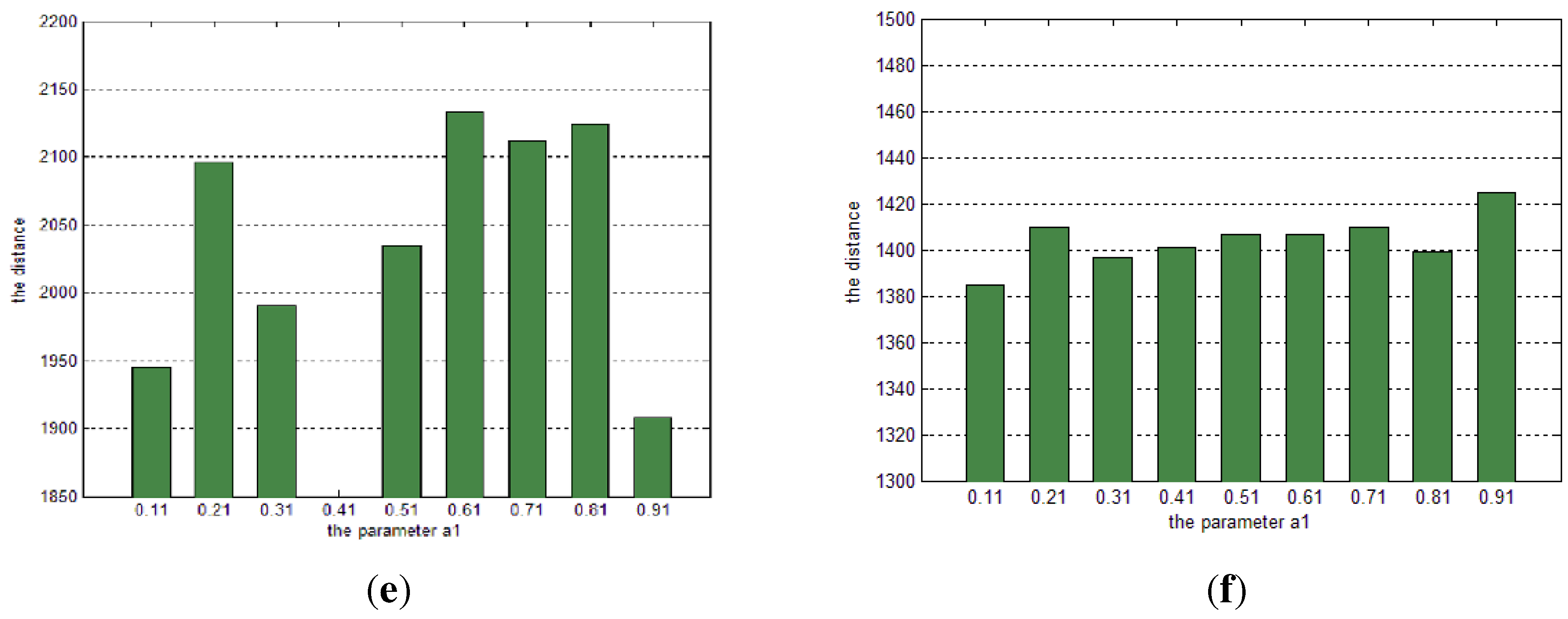
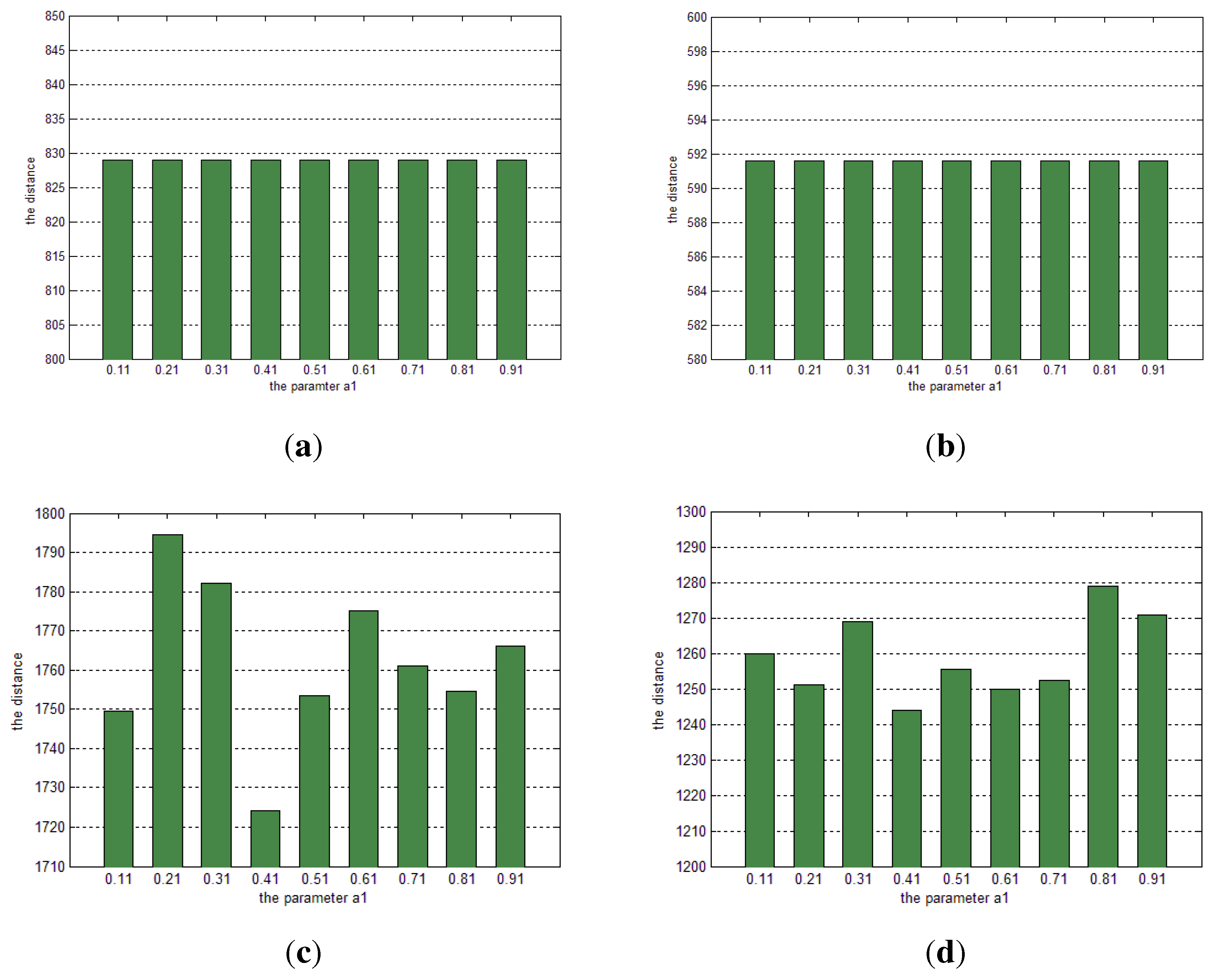
Figure 2, we can make the following conclusion on the parameter analysis of the Insertion Heuristic Algorithm.
- (1)
The parameters can hardly affect the results of C101 and C102. That is because their customer locations are concentrated and the time windows are [0,1,236] and [0,3,390]; it is relatively large.
- (2)
On the other hand, R101 and R102 are largely affected by the parameters. Because their customer locations are a random distribution and the time windows are [0,230] and [0,1,000], it is relatively small. RC101 and RC201 are between the above. In the process of executing, we must set the weights of the parameters according to the data characteristics so that we get the better solution.
Figure 2.
Results comparison of all data sets. (a) C101; (b) C201; (c) R101; (d) R201; (e) RC101; (f) RC201.
Figure 2.
Results comparison of all data sets. (a) C101; (b) C201; (c) R101; (d) R201; (e) RC101; (f) RC201.
5.3. HPSO Performance Comparison by Different Problem Sets
In order to evaluate the proposed HPSO on large-scale problems, we tested on a set of 56 Solomon’s test cases. The aim of the experiments is performance comparison of HPSO for different problem sets in different iteration times, which can test HPSO convergence speed and sensibility to the problem scale. The performance comparison results are shown in
Table 2,
Table 3 and
Table 4.
Table 2,
Table 3 and
Table 4 compare the performance produced by the proposed HPSO in the set of C1, C2, R1, R2, RC1 and RC2 for 100, 200 and 500 iterations. The rate in
Table 2,
Table 3 and
Table 4 expresses the ratio of the difference value of the distance between the best known result and the different iteration time results. Based on these results of
Table 2,
Table 3 and
Table 4, we can make the following conclusion on the HPSO performance of different problem set for solving the VRPTW.
- (1)
In a set of C, the coverage speed to a good solution is fast. It gets an approximately best result by 100 iteration times, many problems of C coverage to the best known results by 200 iteration times and all problems of C coverage to the best known results by 500 iteration times. We can see that HPSO has a better performance on problem set C than Tavakkoli-Moghaddam et al. [
24].
- (2)
In a set of R, the average rate of 100 iteration times is nearly 15% for each problem, the average rate of 200 iteration times is nearly 4% and almost all problems of C coverage to the best known results by 500 iteration times. We can see that HPSO has a better performance on problem set R than Tavakkoli-Moghaddam et al. [
24].
- (3)
In a set of RC, the average rate of 100 iteration times is nearly 13% for each problem, the average rate of 200 iteration times is nearly 6% and almost all problems of C coverage to the best known results by 500 iteration times, except RC101, RC102, RC105, RC107, RC201, RC202, RC203 and RC207. We can see that HPSO has a better performance on problem set RC than Tavakkoli-Moghaddam et al. [
24].
Table 2.
Comparison of the performance of the proposed HPSO for a set C.
Table 2.
Comparison of the performance of the proposed HPSO for a set C.
| Instance | Best known result | 100 iterations | 200 iterations | 500 iterations |
|---|
| | Vehicle | Distance | Vehicle | Distance | Rate % | Vehicle | Distance | Rate % | Vehicle | Distance | Rate % |
|---|
| C101 | 10 | 828.94 | 10 | 831.01 | 0.25 | 10 | 828.94 | 0.00 | 10 | 828.94 | 0.00 |
| C102 | 10 | 828.94 | 10 | 831.45 | 0.30 | 10 | 828.94 | 0.00 | 10 | 828.94 | 0.00 |
| C103 | 10 | 828.06 | 10 | 830.21 | 0.26 | 10 | 828.68 | 0.08 | 10 | 828.06 | 0.00 |
| C104 | 10 | 824.78 | 10 | 827.77 | 0.36 | 10 | 826.31 | 0.19 | 10 | 824.78 | 0.00 |
| C105 | 10 | 828.94 | 10 | 835.69 | 0.82 | 10 | 828.94 | 0.00 | 10 | 828.94 | 0.00 |
| C106 | 10 | 828.94 | 10 | 834.97 | 0.73 | 10 | 828.94 | 0.00 | 10 | 828.94 | 0.00 |
| C107 | 10 | 828.94 | 10 | 836.74 | 0.94 | 10 | 828.94 | 0.00 | 10 | 828.94 | 0.00 |
| C108 | 10 | 828.94 | 10 | 836.55 | 0.92 | 10 | 828.94 | 0.00 | 10 | 828.94 | 0.00 |
| C109 | 10 | 828.94 | 10 | 835.99 | 0.85 | 10 | 828.94 | 0.00 | 10 | 828.94 | 0.00 |
| C201 | 3 | 591.56 | 3 | 594.11 | 0.43 | 3 | 591.99 | 0.07 | 3 | 591.56 | 0.00 |
| C202 | 3 | 591.56 | 3 | 592.95 | 0.24 | 3 | 591.56 | 0.00 | 3 | 591.56 | 0.00 |
| C203 | 3 | 591.17 | 3 | 592.52 | 0.23 | 3 | 591.31 | 0.02 | 3 | 591.17 | 0.00 |
| C204 | 3 | 590.60 | 3 | 593.62 | 0.51 | 3 | 592.10 | 0.25 | 3 | 590.60 | 0.00 |
| C205 | 3 | 588.88 | 3 | 591.67 | 0.47 | 3 | 589.63 | 0.13 | 3 | 588.88 | 0.00 |
| C206 | 3 | 588.49 | 3 | 592.68 | 0.71 | 3 | 590.12 | 0.28 | 3 | 588.49 | 0.00 |
| C207 | 3 | 588.29 | 3 | 593.74 | 0.93 | 3 | 589.68 | 0.24 | 3 | 588.29 | 0.00 |
| C208 | 3 | 588.32 | 3 | 593.27 | 0.84 | 3 | 592.12 | 0.65 | 3 | 588.32 | 0.00 |
Table 3.
Comparison of the performance of the proposed HPSO for a set R.
Table 3.
Comparison of the performance of the proposed HPSO for a set R.
| Instance | Best known result | 100 iterations | 200 iterations | 500 iterations |
|---|
| | Vehicle | Distance | Vehicle | Distance | Rate % | Vehicle | Distance | Rate % | Vehicle | Distance | Rate % |
|---|
| R101 | 19 | 1645.79 | 20 | 1768.39 | 7.45 | 19 | 1694.21 | 2.94 | 19 | 1684.10 | 2.33 |
| R102 | 17 | 1486.12 | 18 | 1625.32 | 9.37 | 17 | 1602.01 | 7.80 | 17 | 1492.13 | 0.40 |
| R103 | 13 | 1292.68 | 13 | 1435.62 | 11.06 | 13 | 1359.69 | 5.18 | 13 | 1300.10 | 0.57 |
| R104 | 9 | 1007.24 | 9 | 1289.96 | 28.07 | 9 | 1109.32 | 10.14 | 9 | 1007.24 | 0.00 |
| R105 | 14 | 1377.11 | 15 | 1541.21 | 11.92 | 14 | 1487.84 | 8.04 | 14 | 1380.14 | 0.22 |
| R106 | 12 | 1251.98 | 13 | 1398.65 | 11.72 | 12 | 1296.37 | 3.55 | 12 | 1257.63 | 0.45 |
| R107 | 10 | 1104.66 | 11 | 1232.28 | 11.55 | 10 | 1164.21 | 5.39 | 10 | 1104.66 | 0.00 |
| R108 | 9 | 960.88 | 10 | 1012.96 | 5.42 | 9 | 1002.64 | 4.35 | 9 | 960.88 | 0.00 |
| R109 | 11 | 1194.73 | 12 | 1301.27 | 8.92 | 11 | 1259.68 | 5.44 | 11 | 1200.01 | 0.44 |
| R110 | 10 | 1118.59 | 10 | 1241.74 | 11.01 | 10 | 1187.69 | 6.18 | 10 | 1118.59 | 0.00 |
| R111 | 10 | 1096.72 | 10 | 1279.68 | 16.68 | 10 | 1124.08 | 2.50 | 10 | 1099.78 | 0.28 |
| R112 | 9 | 982.14 | 10 | 1214.19 | 23.63 | 9 | 1023.15 | 4.18 | 9 | 984.10 | 0.20 |
| R201 | 4 | 1253.37 | 4 | 1458.35 | 16.35 | 4 | 1296.39 | 3.43 | 4 | 1253.37 | 0.00 |
| R202 | 3 | 1191.70 | 3 | 1354.96 | 13.70 | 3 | 1264.54 | 6.11 | 3 | 1196.39 | 0.39 |
| R203 | 3 | 939.54 | 3 | 1102.39 | 17.33 | 3 | 978.98 | 4.20 | 3 | 941.58 | 0.22 |
| R204 | 2 | 825.52 | 2 | 1021.97 | 23.80 | 2 | 874.18 | 5.89 | 2 | 825.52 | 0.00 |
| R205 | 3 | 994.42 | 3 | 1124.02 | 3.03 | 3 | 1032.68 | 3.85 | 3 | 996.85 | 0.24 |
| R206 | 3 | 906.14 | 3 | 1168.38 | 28.94 | 3 | 965.47 | 6.55 | 3 | 906.14 | 0.00 |
| R207 | 2 | 893.33 | 2 | 1038.76 | 16.28 | 2 | 938.51 | 5.06 | 2 | 893.33 | 0.00 |
| R208 | 2 | 726.75 | 2 | 874.10 | 20.28 | 2 | 745.65 | 2.60 | 2 | 726.75 | 0.00 |
| R209 | 3 | 909.16 | 3 | 1094.52 | 20.39 | 3 | 934.74 | 2.81 | 3 | 910.85 | 0.19 |
| R210 | 3 | 939.34 | 3 | 1034.67 | 10.15 | 3 | 968.14 | 3.07 | 3 | 939.34 | 0.00 |
| R211 | 2 | 892.71 | 2 | 968.98 | 8.54 | 2 | 913.61 | 2.34 | 2 | 892.71 | 0.00 |
Table 4.
Comparison of the performance of the proposed HPSO for a set RC.
Table 4.
Comparison of the performance of the proposed HPSO for a set RC.
| Instance | Best known result | 100 iterations | 200 iterations | 500 iterations |
|---|
| | Vehicle | Distance | Vehicle | Distance | Rate % | Vehicle | Distance | Rate % | Vehicle | Distance | Rate % |
|---|
| RC101 | 14 | 1696.94 | 15 | 1869.32 | 10.16 | 15 | 1786.32 | 5.27 | 14 | 1739.68 | 5.70 |
| RC102 | 12 | 1554.75 | 13 | 1754.98 | 12.88 | 13 | 1652.32 | 6.28 | 12 | 1605.25 | 3.25 |
| RC103 | 11 | 1261.67 | 12 | 1475.52 | 16.95 | 11 | 1387.63 | 9.98 | 11 | 1261.67 | 0.00 |
| RC104 | 10 | 1135.48 | 11 | 1296.36 | 14.17 | 10 | 1196.68 | 5.39 | 10 | 1135.48 | 0.00 |
| RC105 | 13 | 1629.44 | 14 | 1872.39 | 14.91 | 14 | 1796.31 | 10.24 | 13 | 1729.84 | 6.18 |
| RC106 | 11 | 1424.73 | 12 | 1596.37 | 12.05 | 11 | 1496.39 | 5.03 | 11 | 1424.73 | 0.00 |
| RC107 | 11 | 1230.48 | 12 | 1421.01 | 15.48 | 12 | 1301.21 | 5.75 | 11 | 1277.46 | 3.82 |
| RC108 | 10 | 1139.82 | 10 | 1396.39 | 22.51 | 10 | 1198.69 | 5.17 | 10 | 1139.82 | 0.00 |
| RC201 | 4 | 406.91 | 4 | 1742.39 | 23.85 | 4 | 1510.36 | 7.35 | 4 | 1486.02 | 5.62 |
| RC202 | 3 | 1367.09 | 3 | 1584.24 | 15.88 | 3 | 1421.35 | 3.97 | 3 | 1399.69 | 2.39 |
| RC203 | 3 | 1049.62 | 3 | 1257.47 | 19.80 | 3 | 1187.10 | 13.10 | 3 | 1055.25 | 0.54 |
| RC204 | 3 | 798.41 | 3 | 902.10 | 12.99 | 3 | 809.69 | 1.41 | 3 | 798.41 | 0.00 |
| RC205 | 4 | 1297.19 | 4 | 1547.96 | 19.33 | 4 | 1352.25 | 4.25 | 4 | 1297.19 | 0.00 |
| RC206 | 3 | 1146.32 | 3 | 1321.17 | 15.25 | 3 | 1169.39 | 2.01 | 3 | 1146.32 | 0.00 |
| RC207 | 3 | 1061.14 | 3 | 1268.39 | 19.53 | 3 | 1186.39 | 11.80 | 3 | 1076.96 | 1.49 |
| RC208 | 3 | 828.14 | 3 | 1000.14 | 20.77 | 3 | 896.10 | 8.21 | 3 | 828.14 | 0.00 |
5.4. Comparison Results of HPSO and PSO
In HPSO, in order to avoid falling into the local optimum, this paper uses COA and Gaussian mutation. In order to add the number of particles in the early stage and to accelerate the searching speed in solution space, this paper uses COA to reinitialize the particle swarm. To verify results, this section makes experiments to compare the HPSO and basic PSO and tests the effect of COA in HPSO. The results are shown in
Table 5.
Table 5 compares the performance produced by the proposed HPSO and basic PSO in the set C1, R1 and RC1. The run-time in
Table 5 expresses the solving time of problems by HPSO or PSO. The rate in
Table 5 expresses the ration of different value of distance between the best known result and HPSO or PSO results. If the rate value is negative, it means that the distance value of HPSO or PSO is shorter than the best known results. If the rate value is a positive number, it means that the distance value of HPSO or PSO is bigger than the best known results. Based on these results of
Table 5, we can make the following conclusion on the performance of HPSO and PSO on solving the VRPTW.
- (1)
HPSO can get all the best known results, and sometimes, it gets better results than the best known result, such as for problems R101, R103, R105, R106 and RC101; while basic PSO can hardly cover the best known results for almost all problems of C1, R1 and RC1. We can see that HPSO has better performance than basic PSO.
- (2)
HPSO covers the best known results at nearly two minutes for R1, one minute for C1 and at most three minutes for RC1. PSO covers its best results at least three minutes for R1, two minutes for C1 and four minutes for RC1. We can see that COA can effectively accelerate the searching speed in solution space, and the HPSO has better performance coverage speed than basic PSO.
Table 5.
Comparison of the performance of HPSO and PSO.
Table 5.
Comparison of the performance of HPSO and PSO.
| Instance | Best known result | HPSO | PSO |
|---|
| | Vehicle | Distance | Vehicle | Distance | Run-time (s) | Rate % | Vehicle | Distance | Run-time (s) | Rate % |
|---|
| R101 | 19 | 1645.79 | 19 | 1640.32 | 135.36 | -0.33 | 19 | 1689.66 | 196.35 | 2.67 |
| R102 | 17 | 1486.12 | 17 | 1486.12 | 123.96 | 0.00 | 17 | 1497.47 | 186.47 | 0.76 |
| R103 | 13 | 1292.68 | 13 | 1286.96 | 116.35 | -0.44 | 13 | 1329.65 | 175.85 | 2.86 |
| R104 | 9 | 1007.24 | 9 | 1007.24 | 114.24 | 0.00 | 9 | 1087.29 | 168.96 | 7.95 |
| R105 | 14 | 1377.11 | 14 | 1369.11 | 125.85 | -0.58 | 14 | 1489.96 | 172.32 | 7.98 |
| R106 | 12 | 1251.98 | 12 | 1248.47 | 121.18 | -0.28 | 12 | 1306.65 | 169.69 | 4.37 |
| R107 | 10 | 1104.66 | 10 | 1104.66 | 114.96 | 0.00 | 10 | 1254.19 | 164.32 | 13.54 |
| R108 | 9 | 960.88 | 9 | 960.88 | 109.69 | 0.00 | 9 | 990.74 | 161.85 | 3.11 |
| R109 | 11 | 1194.73 | 11 | 1194.73 | 115.65 | 0.00 | 11 | 1201.78 | 167.98 | 0.59 |
| R110 | 10 | 1118.59 | 10 | 1118.59 | 112.39 | 0.00 | 10 | 1189.63 | 164.91 | 6.35 |
| R111 | 10 | 1096.72 | 10 | 1096.72 | 116.21 | 0.00 | 10 | 1096.72 | 172.21 | 0.00 |
| R112 | 9 | 982.14 | 9 | 982.14 | 105.24 | 0.00 | 9 | 982.14 | 168.97 | 0.00 |
| C101 | 10 | 828.94 | 10 | 828.94 | 58.65 | 0.00 | 10 | 838.64 | 102.64 | 1.17 |
| C102 | 10 | 828.94 | 10 | 828.94 | 59.63 | 0.00 | 10 | 859.06 | 106.39 | 3.63 |
| C103 | 10 | 828.06 | 10 | 828.06 | 61.24 | 0.00 | 10 | 828.06 | 100.23 | 0.00 |
| C104 | 10 | 824.78 | 10 | 824.78 | 52.47 | 0.00 | 10 | 842.98 | 99.68 | 2.20 |
| C105 | 10 | 828.94 | 10 | 828.94 | 61.03 | 0.00 | 10 | 858.32 | 109.64 | 3.54 |
| C106 | 10 | 828.94 | 10 | 828.94 | 60.14 | 0.00 | 10 | 863.21 | 108.47 | 4.13 |
| C107 | 10 | 828.94 | 10 | 828.94 | 61.07 | 0.00 | 10 | 835.69 | 106.85 | 0.81 |
| C108 | 10 | 828.94 | 10 | 828.94 | 57.41 | 0.00 | 10 | 839.89 | 102.36 | 1.32 |
| C109 | 10 | 828.94 | 10 | 828.94 | 56.39 | 0.00 | 10 | 828.94 | 100.29 | 0.00 |
| RC101 | 14 | 1696.94 | 14 | 1689.36 | 165.21 | -0.45 | 14 | 1851.09 | 269.65 | 9.08 |
| RC102 | 12 | 1554.75 | 12 | 1554.75 | 159.21 | 0.00 | 12 | 1618.47 | 256.32 | 4.10 |
| RC103 | 11 | 1261.67 | 11 | 1261.67 | 138.69 | 0.00 | 11 | 1326.41 | 259.34 | 5.13 |
| RC104 | 10 | 1135.48 | 10 | 1135.48 | 135.21 | 0.00 | 10 | 1169.09 | 241.17 | 2.96 |
| RC105 | 13 | 1629.44 | 13 | 1629.44 | 168.95 | 0.00 | 13 | 1684.46 | 239.69 | 3.50 |
| RC106 | 11 | 1424.73 | 11 | 1424.73 | 154.12 | 0.00 | 11 | 1557.02 | 241.73 | 9.28 |
| RC107 | 11 | 1230.48 | 11 | 1230.48 | 139.68 | 0.00 | 11 | 1247.65 | 235.25 | 1.40 |
| RC108 | 10 | 1139.82 | 10 | 1139.82 | 135.87 | 0.00 | 10 | 1293.21 | 231.04 | 13.46 |
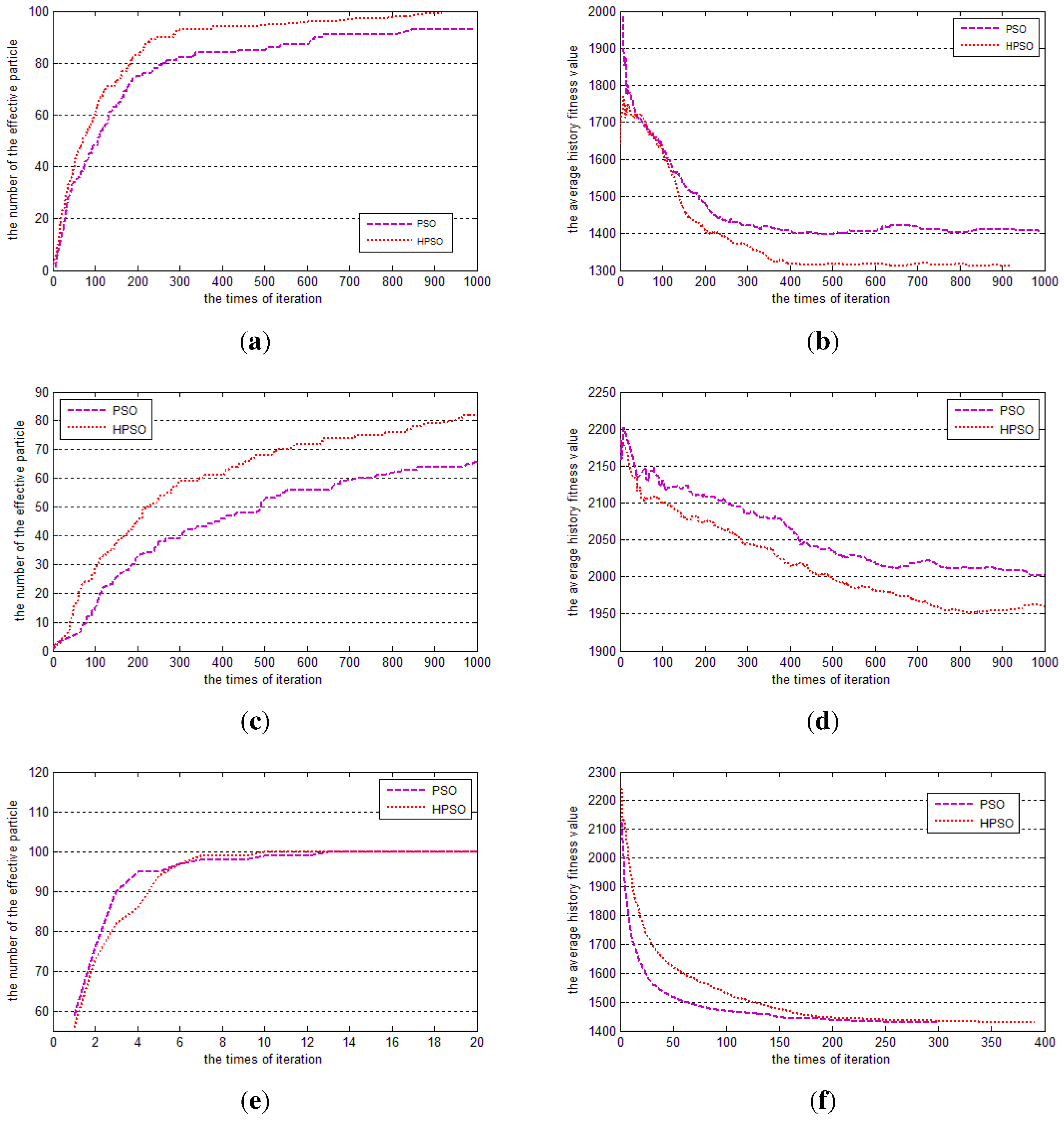
Because the number of the vehicles and routes in different data sets are different, this paper only chooses R201, RC101 and RC201 to make an experiment. The comparisons of the number and the average optimal fitness value in history of the effective particle are shown as
Figure 3. From the data of
Figure 3, it is easy to get HPSO better than PSO. Although, in RC101, the solution of HPSO is worse than PSO. The number of effective particles and the average optimal fitness value in history of HPSO are better than PSO. This shows that HPSO is more effective.
Figure 3.
The comparisons of the number and the average optimal fitness value in the history of the effective particle. (a) the number of effective particles of R201; (b) the average optimal fitness value in history of R201; (c) the number of effective particles of RC101; (d) the average optimal fitness value in history of RC101; (e) the number of effective particles of RC201; (f) the average optimal fitness value in history of RC201.
5.5. Comparison Result of HPSO with Other State-of-the-art Methods
In order to compare the efficiency of different algorithms to VRPTW, The state-of-the-art method of Goal Programming and Genetic Algorithm (GPGA) [
28], Improved Large Neighborhood Search (I-LNS) [
22] and Ant Colony Optimization Hybridized with Insertion Heuristics (ACO-IH) [
25] are used to compare HPSO. The results of comparison experiments of VRPTW are shown in
Table 6,
Table 7 and
Table 8. The rate in
Table 6,
Table 7 and
Table 8 expresses the ratio of the difference value of the distance between HPSO and other state-of-the-art methods. If the rate value is negative, it means that the distance value of HPSO is shorter than other state-of-the-art methods. If the rate value is a positive number, it means that the distance value of HPSO is bigger than other state-of-the-art methods. Based on these results of
Table 6,
Table 7 and
Table 8, we can make the following conclusion on the effectiveness of the HPSO approach for solving the VRPTW.
Table 6.
Comparison results of different methods for vehicle routing problem with time windows (VRPTW) of R1.
Table 6.
Comparison results of different methods for vehicle routing problem with time windows (VRPTW) of R1.
| Instance | HPSO | Best known results | GPGA | I-LNS | ACO-Ih |
|---|
| | Vehicle | Distance | CPU(s) | Vehicle | Distance | Rate % | Vehicle | Distance | Rate % | Vehicle | Distance | Rate % | Vehicle | Distance | Rate % |
|---|
| R101 | 19 | 1640.32 | 135.36 | 19 | 1645.79 | -0.33 | 19 | 1677.00 | -2.44 | 18 | 1612.29 | 1.71 | 19 | 1650.80 | -0.64 |
| R102 | 17 | 1486.12 | 123.96 | 17 | 1486.12 | 0.00 | 18 | 1511.80 | -1.73 | 16 | 1473.41 | 0.86 | 17 | 1486.12 | 0.00 |
| R103 | 13 | 1286.96 | 116.35 | 13 | 1292.68 | -0.44 | 14 | 1287.00 | -0.03 | 12 | 1279.37 | 0.59 | 13 | 1292.68 | -0.44 |
| R104 | 9 | 1007.24 | 114.24 | 9 | 1007.24 | 0.00 | 10 | 974.24 | 3.27 | 10 | 1025.47 | -1.81 | 9 | 1007.31 | -0.01 |
| R105 | 14 | 1369.11 | 125.85 | 14 | 1377.11 | -0.58 | 15 | 1424.60 | -4.05 | 14 | 1377.95 | -0.65 | 14 | 1377.11 | -0.58 |
| R106 | 12 | 1248.47 | 121.18 | 12 | 1251.98 | -0.28 | 13 | 1270.30 | -1.75 | 12 | 1276.48 | -2.24 | 12 | 1252.03 | -0.29 |
| R107 | 10 | 1104.66 | 114.96 | 10 | 1104.66 | 0.00 | 11 | 1108.80 | -0.38 | 11 | 1153.86 | -4.45 | 10 | 1104.66 | 0.00 |
| R108 | 9 | 960.88 | 109.69 | 9 | 960.88 | 0.00 | 10 | 971.91 | -1.15 | 10 | 990.82 | -3.12 | 9 | 960.88 | 0.00 |
| R109 | 11 | 1194.73 | 115.65 | 11 | 1194.73 | 0.00 | 12 | 1212.30 | -1.47 | 12 | 1179.73 | 1.26 | 11 | 1194.73 | 0.00 |
| R110 | 10 | 1118.59 | 112.39 | 10 | 1118.59 | 0.00 | 12 | 1156.5 | -3.39 | 11 | 1113.10 | 0.49 | 10 | 1118.84 | -0.02 |
| R111 | 10 | 1096.72 | 116.21 | 10 | 1096.72 | 0.00 | 11 | 1111.9 | -1.38 | 11 | 1155.39 | -5.35 | 10 | 1096.73 | 0.00 |
| R112 | 9 | 982.14 | 105.24 | 9 | 982.14 | 0.00 | 10 | 1036.9 | -5.58 | 10 | 981.46 | 0.07 | 9 | 985.28 | -0.32 |
Table 7.
Comparison results of different methods for VRPTW of C1.
Table 7.
Comparison results of different methods for VRPTW of C1.
| Instance | HPSO | Best known results | GPGA | I-LNS | ACO-Ih |
|---|
| | Vehicle | Distance | CPU(s) | Vehicle | Distance | Rate % | Vehicle | Distance | Rate % | Vehicle | Distance | Rate % | Vehicle | Distance | Rate % |
|---|
| C101 | 10 | 828.94 | 58.65 | 10 | 828.94 | 0.00 | 10 | 828.94 | 0.00 | 10 | 828.94 | 0.00 | 10 | 828.94 | 0.00 |
| C102 | 10 | 828.94 | 59.63 | 10 | 828.94 | 0.00 | 10 | 828.94 | 0.00 | 10 | 828.94 | 0.00 | 10 | 828.94 | 0.00 |
| C103 | 10 | 828.06 | 61.24 | 10 | 828.06 | 0.00 | 10 | 828.06 | 0.00 | 10 | 839.37 | -1.37 | 10 | 828.06 | 0.00 |
| C104 | 10 | 824.78 | 52.47 | 10 | 824.78 | 0.00 | 10 | 824.78 | 0.00 | 10 | 838.98 | -1.72 | 10 | 824.78 | 0.00 |
| C105 | 10 | 828.94 | 61.03 | 10 | 828.94 | 0.00 | 10 | 828.94 | 0.00 | 10 | 828.94 | 0.00 | 10 | 828.94 | 0.00 |
| C106 | 10 | 828.94 | 60.14 | 10 | 828.94 | 0.00 | 10 | 828.94 | 0.00 | 10 | 842.10 | -1.59 | 10 | 828.94 | 0.00 |
| C107 | 10 | 828.94 | 61.07 | 10 | 828.94 | 0.00 | 10 | 828.94 | 0.00 | 10 | 828.94 | 0.00 | 10 | 828.94 | 0.00 |
| C108 | 10 | 828.94 | 57.41 | 10 | 828.94 | 0.00 | 10 | 828.94 | 0.00 | 10 | 832.74 | -0.46 | 10 | 828.94 | 0.00 |
| C109 | 10 | 828.94 | 56.39 | 10 | 828.94 | 0.00 | 10 | 828.94 | 0.00 | 10 | 828.94 | 0.00 | 10 | 828.94 | 0.00 |
- (1)
The solution quality computed by HPSO can approximate the best known results well. If the travel distances and the number of used vehicles are taken into account seriously, the HPSO can almost get the best results of C1, R1 and RC1.
- (2)
Comparing with the results generated by GPGA, I-LNS and ACO-IH, the results of HPSO are almost better than them. The average CPU times of HPSO are less than 3 min. The results are hard to systematically compare with other state-of-the-art methods, because there are big differences in the run environments.
Table 8.
Comparison results of different methods for VRPTW of RC1.
Table 8.
Comparison results of different methods for VRPTW of RC1.
| Instance | HPSO | Best known results | GPGA | I-LNS | ACO-Ih |
|---|
| | Vehicle | Distance | CPU(s) | Vehicle | Distance | Rate % | Vehicle | Distance | Rate % | Vehicle | Distance | Rate % | Vehicle | Distance | Rate % |
|---|
| RC101 | 14 | 1689.36 | 165.21 | 14 | 1696.94 | -0.45 | 15 | 1690.60 | -0.07 | 15 | 1671.54 | 1.06 | 14 | 1696.94 | -0.45 |
| RC102 | 12 | 1554.75 | 159.21 | 12 | 1554.75 | 0.00 | 14 | 1509.40 | 2.92 | 13 | 1447.14 | 6.92 | 12 | 1554.75 | 0.00 |
| RC103 | 11 | 1261.67 | 138.69 | 11 | 1261.67 | 0.00 | 12 | 1331.80 | -5.56 | 11 | 1313.79 | -4.13 | 11 | 1262.02 | -0.03 |
| RC104 | 10 | 1135.48 | 135.21 | 10 | 1135.48 | 0.00 | 11 | 1177.20 | -3.67 | 11 | 1163.54 | -2.47 | 10 | 1135.48 | 0.00 |
| RC105 | 13 | 1629.44 | 168.95 | 13 | 1629.44 | 0.00 | 15 | 1611.50 | 1.10 | 13 | 1502.48 | 7.79 | 13 | 1629.44 | 0.00 |
| RC106 | 11 | 1424.73 | 154.12 | 11 | 1424.73 | 0.00 | 13 | 1437.60 | -0.90 | 12 | 1406.25 | 1.30 | 11 | 1424.73 | 0.00 |
| RC107 | 11 | 1230.48 | 139.68 | 11 | 1230.48 | 0.00 | 11 | 1222.10 | 0.68 | 11 | 1278.96 | -3.94 | 11 | 1230.48 | 0.00 |
| RC108 | 10 | 1139.82 | 135.87 | 10 | 1139.82 | 0.00 | 11 | 1156.50 | -1.46 | 11 | 1172.83 | -2.90 | 10 | 1139.82 | 0.00 |
5.6. A Real-World Numerical Example
A real-world numerical example is provided here to illustrate the effectiveness of HPSO. The data of Yunda Expressage Company of Wuhan City is used to test the sensitivity of the algorithm to the specimen data. One-day data of the Yunda Expressage Company of Wuhan City of Hongshang district is transformed as a Solomon problem set format, which is shown in
Table 9. Yunda Expressage Company of Wuhan City has 10 vehicles. They have 60 delivery nodes in Hongshang district. The delivery nodes can be defined as the customers of Solomon problem data set. We use HPSO to solve this real-world numerical example, and the computing result is shown in
Table 10. We use other state-of-the-art methods to solve this example, and the comparison result of HPSO with other state-of-the-art methods is shown in
Table 11. Based on these results of
Table 9,
Table 10 and
Table 11, we can make the following conclusion on the performance of the HPSO and other state-of-the-art methods on solving a real-world numerical example.
Table 9.
One-day data of Yunda expressage company of Wuhan city.
Table 9.
One-day data of Yunda expressage company of Wuhan city.
| Delivery node | N1 | N2 | N3 | N4 | N5 | N6 | N7 | N8 | N9 | N10 | N11 | N12 | N13 | N14 | N15 |
| XCOORD | 90 | 50 | 120 | 60 | 20 | 10 | 15 | 30 | 180 | 60 | 20 | 10 | 80 | 70 | 120 |
| YCOORD | 120 | 60 | 20 | 30 | 120 | 150 | 30 | 170 | 25 | 120 | 100 | 150 | 150 | 60 | 100 |
| DEMAN | 24 | 10 | 5 | 10 | 5 | 10 | 15 | 10 | 6 | 5 | 6 | 4 | 6 | 6 | 10 |
| READY TIME | 0 | 10 | 12 | 2 | 6 | 4 | 2 | 2 | 6 | 2 | 4 | 10 | 10 | 2 | 6 |
| DUE TIME | 48 | 28 | 24 | 18 | 18 | 24 | 12 | 16 | 24 | 16 | 24 | 24 | 24 | 12 | 18 |
| SERVICE TIME | 1 | 2 | 1 | 2 | 1 | 2 | 1 | 1 | 1 | 1 | 1 | 1 | 2 | 1 | 1 |
| Delivery node | N16 | N17 | N18 | N19 | N20 | N21 | N22 | N23 | N24 | N25 | N26 | N27 | N28 | N29 | N30 |
| XCOORD | 120 | 30 | 120 | 60 | 120 | 180 | 170 | 100 | 25 | 30 | 65 | 160 | 150 | 30 | 65 |
| YCOORD | 90 | 60 | 80 | 50 | 10 | 160 | 30 | 180 | 125 | 155 | 185 | 110 | 10 | 185 | 95 |
| DEMAN | 10 | 5 | 5 | 14 | 10 | 2 | 6 | 10 | 16 | 10 | 10 | 10 | 20 | 5 | 12 |
| READY TIME | 0 | 0 | 10 | 15 | 10 | 0 | 15 | 2 | 10 | 12 | 24 | 2 | 6 | 10 | 5 |
| DUE TIME | 24 | 12 | 24 | 24 | 36 | 24 | 30 | 24 | 24 | 24 | 48 | 16 | 14 | 24 | 15 |
| SERVICE TIME | 2 | 1 | 1 | 4 | 1 | 1 | 1 | 1 | 1 | 1 | 1 | 1 | 1 | 1 | 1 |
| Delivery node | N31 | N32 | N33 | N34 | N35 | N36 | N37 | N38 | N39 | N40 | N41 | N42 | N43 | N44 | N45 |
| XCOORD | 75 | 40 | 175 | 45 | 105 | 45 | 65 | 130 | 180 | 160 | 125 | 105 | 55 | 170 | 120 |
| YCOORD | 35 | 80 | 25 | 35 | 120 | 150 | 15 | 170 | 125 | 120 | 45 | 115 | 40 | 60 | 50 |
| DEMAN | 24 | 10 | 5 | 10 | 5 | 10 | 15 | 10 | 6 | 5 | 6 | 4 | 6 | 6 | 10 |
| READY TIME | 0 | 10 | 12 | 2 | 6 | 4 | 2 | 2 | 6 | 2 | 4 | 10 | 10 | 2 | 6 |
| DUE TIME | 48 | 28 | 24 | 18 | 18 | 24 | 12 | 16 | 24 | 16 | 24 | 24 | 24 | 12 | 18 |
| SERVICE TIME | 1 | 2 | 1 | 2 | 1 | 2 | 1 | 1 | 1 | 1 | 1 | 1 | 2 | 1 | 1 |
| Delivery node | N46 | N47 | N48 | N49 | N50 | N51 | N52 | N53 | N54 | N55 | N56 | N57 | N58 | N59 | N60 |
| XCOORD | 35 | 45 | 120 | 75 | 120 | 180 | 170 | 100 | 25 | 130 | 75 | 45 | 135 | 75 | 105 |
| YCOORD | 95 | 10 | 95 | 45 | 115 | 55 | 45 | 75 | 85 | 105 | 95 | 120 | 45 | 50 | 105 |
| DEMAN | 10 | 5 | 5 | 14 | 10 | 2 | 6 | 10 | 16 | 10 | 10 | 5 | 5 | 14 | 10 |
| READY TIME | 0 | 0 | 10 | 15 | 10 | 0 | 15 | 2 | 10 | 12 | 0 | 0 | 10 | 15 | 10 |
| DUE TIME | 24 | 12 | 24 | 24 | 36 | 24 | 30 | 24 | 24 | 24 | 24 | 12 | 24 | 24 | 36 |
| SERVICE TIME | 2 | 1 | 1 | 4 | 1 | 1 | 1 | 1 | 1 | 1 | 2 | 1 | 1 | 4 | 1 |
Table 10.
The computing result of the real-word numerical example by HPSO.
Table 10.
The computing result of the real-word numerical example by HPSO.
| Vehicle ID | The Amount of delivery node | delivery node |
|---|
| V01 | 8 | [N1] [N13] [N14] [N35] [N42] [N49] [N53] [N60] |
| V02 | 7 | [N15] [N16] [N18] [N45] [N48] [N50] [N55] |
| V03 | 11 | [N8] [N9] [N21] [N23] [N27] [N33] [N39] [N40] [N44][N51][N52] |
| V04 | 11 | [N2] [N4] [N17] [N19] [N30] [N32] [N34] [N43] [N46] [N47] [N59] |
| V05 | 6 | [N5] [N6] [N11] [N12] [N24] [N25] |
| V06 | 6 | [N3] [N20] [N28] [N38] [N41] [N58] |
| V07 | 7 | [N10] [[N26] [N29] [N31] [N36] [N56] [N57] |
| V08 | 4 | [N7] [N22] [N37] [N54] |
| V09 | | |
| V10 | | |
- (1)
HPSO coverage a good solution, which can satisfy the company’s requirement. HPSO can get less distance than almost all other state-of-the-art methods, just a little bigger than the LNS method, but the LNS method needs more vehicles to support it.
- (2)
HPSO coverage to a satisfied solution by least iteration times than other state-of-the-art methods. It uses the least run-time times to solve this example compared to other state-of-the-art methods.
- (3)
In conclusion, HPSO achieves better performance than other state-of-the-art methods on solving real-world VRPTW.
Table 11.
The result of comparison experiments of the real-world numerical example.
Table 11.
The result of comparison experiments of the real-world numerical example.
| Algorithm | Coverage iteration times | Run-time (s) | Vehicle | Distance |
|---|
| HPSO | 478 | 121.36 | 8 | 1687.28 |
| PSO | 1586 | 298.68 | 10 | 1965.24 |
| GPGA | 798 | 187.54 | 9 | 1712.98 |
| SA | 1025 | 247.87 | 10 | 1701.41 |
| TS | 981 | 199.68 | 10 | 1689.10 |
| ACO-IH | 1014 | 245.63 | 9 | 1754.98 |
| I-LNS | 765 | 178.69 | 9 | 1685.24 |
6. Conclusions
VRPTW has drawn great interest in the field of vehicle routing. The research area of the problem also expanded to water carriage, aviation, logistics, industrial management and communication. Most researchers use heuristic evolutionary algorithms to solve it. However, the principles of these heuristic algorithms are mostly complex and need more optimization work. This paper proposes a hybrid PSO algorithm, combining the chaos optimization algorithm and the heuristic algorithm, with the purpose of improving the number of effective particles and avoiding falling into local optimization.
The experiments mainly analyze the influence of the insertion heuristic algorithm parameters and comparison of HPSO with state-of-the-art methods. From the experiments, it concludes that:
- (1)
it is necessary to set the weights for the parameters according to the characteristics of customer locations and time windows. When there are feasible solutions, using the Chaos Optimization Algorithm to re-initialize the particle swarm can speed up the convergence rate. Using CAO and Gaussian mutation can further avoid falling into the local optimum.
- (2)
Using the Solomon benchmark, HPSO achieves much better performance than the other state-of-the-art methods in converging speed and solutions.
- (3)
Using a real-world numerical example, HPSO covers a better solution than the other state-of-the-art methods, and its coverage iteration times and run-time times are also the least.
Although HPSO for VRPTW obtains satisfactory achievements, there are still some spaces for improvement, such as how to effectively construct the initial solution and how to precisely judge the local optimal solution. These would be explored in our future work.


