
Polyprotic Acids and Beyond—An Algebraic Approach

Umwelt- und Ingenieurtechnik GmbH Dresden (UIT), Zum Windkanal 21, 01109 Dresden, Germany
Chemistry 2021, 3(2), 454-508; https://doi.org/10.3390/chemistry3020034
Submission received: 3 March 2021
/
Revised: 18 March 2021
/
Accepted: 19 March 2021
/
Published: 7 April 2021
(This article belongs to the Section Theoretical and Computational Chemistry)
Abstract
:For an N-protic acid–base system, the set of nonlinear equations (i.e., mass action and balance laws) provides a simple analytical solution/formula for any integer N ≥ 1. The approach is applicable for the general case of zwitterionic acids HNA+Z (e.g., amino acids, NTA, and EDTA), which includes (i) the “ordinary acids” as a special case (Z = 0) and (ii) surface complexation. Examples are presented for N = 1 to 6. The high-N perspective allows the classification of equivalence points (including isoionic and isoelectric points). Principally, there are two main approaches to N-protic acids: one from hydrochemistry and one “outside inorganic hydrochemistry”. They differ in many ways: the choice of the reference state (either HNA or A−N), the reaction type (dissociation or association), the type/nature of the acidity constants, and the structure of the formulas. Once the (nonlinear) conversion between the two approaches is established, we obtain a systematics of acidity constants (macroscopic, microscopic, cumulative, and Simms). Finally, from the viewpoint of statistical mechanics (canonical isothermal–isobaric ensemble), buffer capacities, buffer intensities, and higher pH derivatives are actually fluctuations in the form of variance, skewness, and kurtosis.
1. Introduction
1.1. State of the Art
The subject of acid–base equilibria is covered in an extensive bibliography, usually focusing on mono- and diprotic acids, which is the entry point to understanding chemical equilibrium reactions per se. The list of classical textbooks and monographies is long and stems from various subfields, such as hydrochemistry [1,2,3] as well as general and analytical chemistry [4,5,6,7]. This is accompanied with several modeling approaches, e.g., [8,9,10].
For the general case of aquatic systems (as mixtures of any number of acids and bases plus solid and gaseous phases), there are two prototypes of numerical approaches: (i) models that are based on the law of mass action (e.g., PhreeqC [11] and many others) and (ii) models that are based on Gibbs energy minimization (GEM) [12,13].
The mathematical description of polyprotic acids (with N ≥ 3) is a special topic that extends the traditional view on acid–base reactions. Algebraic equations are presented in [14,15,16,17,18,19,20]; their application to titration and buffer capacities can be found in [21,22,23,24] and in [25,26,27,28,29,30]. Many of the developments come from areas outside conventional hydrochemistry (e.g., org/bio/med chemistry), which is the playground of proton-binding macromolecules such as nucleic acids and fulvic/humic acids. This also encourages a statistical description [31,32,33,34].
There are two principal ways of mathematical description: (i) the hydrochemical approach (based on dissociation reactions with reference state HNA) and (ii) the approach employed in organic and biochemistry (based on association reactions with reference state A−N). The present review follows the first approach; the interrelation with the second approach is established in Section 2.5. The latter provides an overview of different types of equilibrium constants (macroscopic, cumulative, microscopic) used today in acid–base theory—see Section 2.5.7.
The question whether a polyprotic acid HNA can be represented as a sum of N monoprotic acids is answered in Section 2.5.5 and Section 2.5.6 by factorizing the partition function of the canonical isothermal–isobaric ensemble. This is equivalent to the “quasiparticle-like” concept of N noninteracting proton-binding sites, known as decoupled sites representation (DSR) [33,34].
Titration and buffer capacities are summarized in an excellent review article by Asuero and Michałowski [26]. This and other papers [24,25,26,27,28,29,30] rely on association reactions (with reference state A−N), so one has to be careful when comparing the formulas with the present approach. Additionally, most of these papers take the dilution during titration into account by explicitly using the volume of the titrant. This effect is ignored in this review to keep the formulas simple.
1.2. Motivation
Today, computers solve nonlinear systems numerically in the shortest time with high quality, which is a great help in dealing with complex real-world tasks (and we are grateful for that). However, by delegating everything to computers, we sometimes lose the overview of the underlying principles and functional relationships (digital data are too incomplete/imprecise to understand the deeper aspects of reality).
Starting from the laws of mass action and mass/charge balance, a mathematical solution is provided in the form of simple and smooth analytical formulas for acid–base reactions. This is performed for the general case of N-protic acids, where N can be any integer (N ≥ 1). The approach applies to the broad class of zwitterionic acids HNA+Z (amino acids, NTA, EDTA, etc.), which embeds all “ordinary acids” as a special subclass characterized by Z = 0.
There are at least five questions:
- Why do we need equations/formulas for N > 3?
- Is the approach mathematically strict/rigorous?
- What is the difference to standard approaches celebrated in textbooks?
- What does it mean to be a simple and smooth analytical formula?
- This report contains more than 100 formulas. What is the central formula?
Answer 1. Usually (and this is the first that comes to mind) N is a small number: 1, 2 or 3 for monoprotic, diprotic and triprotic acids. However, in reality, there are compounds with more protons (e.g., EDTA with N = 6 in Section 4.1.6 or other macromolecules in biochemistry and/or mixtures thereof). Moreover, when treating N as a variable integer, the equations tell us things that might otherwise be non-obvious (e.g., classification of equivalence points in Section 2.3).
Answer 2. The mathematical derivation is strict/rigorous. For this purpose, it is assumed that the activities (that enter the mass action laws) are replaced by molar concentrations, which is justified either for dilute systems or for non-dilute systems using conditional equilibrium constants (c.f. seawater example in Section 3.3.5). Deviations in the analytical model from numerical activity-based calculations are discussed in Section 3.3.6.
Answer 3. In standard textbooks [1,2,3,4,5,6], an algebraic solution of the acid–base problem is usually provided for diprotic acids (N = 2) in implicit form, namely as a polynomial of degree 4 in x = 10−pH (quartic equation!)—see, e.g., [1] (p. 107) or Equation (46) below. That is the common way to handle the acid–base problem. In the general case of N-protic acids, this procedure leads to polynomials of order N + 2, where, for N > 4, there is principally no algebraic solution (according to the Abel–Ruffini theorem). This dilemma will be avoided in the present approach. However, before we start, let us explain this in another way.
In titration, a titrant (strong base of amount CB) is added to the analyte (N-protic acid with amount CT), resulting in a certain pH value. So, one is tempted to write the pH as a function of CT and CB (or n = CB/CT), that is: pH = pH (analyte, titrant) = pH (CT,CB) or pH = pH (CT, n). However, as mentioned above, these relations cannot be expressed in the form of an explicit function; they only exist implicitly in the form of polynomials of degree N + 2 (see Equation (44)). So we put the whole thing “from head to toe” by providing a strict algebraic solution in the form of the explicit function n = n(CT, pH), or shorter n = n(x). The polynomials are then considered as the inverse task in Section 2.2.3.
Answer 4. “Simple” means that the analytical formula(s) is (are) easy to handle in a Lego-like manner from plain constructs, as summarized in Section 5 at the end of this report. There is no need for programming or root-solving methods. All results/diagrams in this report were created with Excel, and anyone can easily reproduce them.
“Smooth” means that the analytical formula n = n(x)—as well as its building blocks—are infinitely derivable functions that offer calculus in the form of pH derivatives and integrals (a feature that is not possible for numerical solutions/data). The pH derivatives convert buffer capacities to buffer intensities; pH derivatives are also used to identify equivalence points (EPs) as local minima/maxima and/or inflection points.
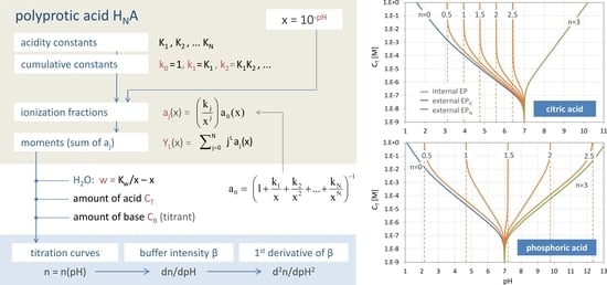
Answer 5. The central formula is the equivalent fraction n = Y1 + w/CT (symbols are explained in the text), which contains all information about the acid–base system in condensed form. As sketched in Figure 1, depending on whether n is a specific discrete number or a real function, different aspects appear: the equivalence points (as special/exceptional equilibrium states) or buffer capacities as “distances” between two equilibrium states. In this report, the function n(x) appears under several names: equivalence fraction, titration function/curve, and normalized buffer capacity (because it measures the distance to EP0).
1.3. Structure of this Report
The report consists of three main parts/sections: (i) the mathematical framework (see also Figure 2), (ii) its application (including the discussion of alternative concepts and common approximations), and (iii) the extension of the approach to zwitterions and surface complexation.
The goal of Section 2 is to bundle a set of N + 3 nonlinear equations into an analytical formula. We start with the 1-component system in Section 2.1, i.e., the N-protic acid itself, which is fully determined by N acidity constants K1 to KN. In Section 2.2, the 1-component system is extended to a 3-component acid–base system, which opens the door to the description of acid–base titrations. After discussion/classification of equivalence points in Section 2.3, buffer capacities and buffer intensities are introduced in Section 2.4. Regarding the connection between the three subsystems in Figure 2, the numbers 1/CT and CB/CT act as “coupling constants” of the acid to the water (autoprotolysis) and to the base. Section 2.5 embeds the present mathematical approach into alternative concepts “outside” traditional hydrochemistry.
In Section 2 and Section 3, example calculations are performed for four common acids listed in Table 1. In fact, the beauty and elegance of the acid–base behavior/equations is best illustrated in diagrams, and this is used extensively in this report. In Section 4, the mathematical description is applied beyond the realm of ordinary acids to zwitterions and surface complexation.
2. Mathematical Framework
2.1. The 1-Component System: N-Protic Acid (HNA)
2.1.1. Notation
An acid is a proton donor; it releases H+ ions (more precisely: H3O+) when dissolved in water:
which is a shorthand for HA(aq) + H2O(l) = H3O+(aq) + A−(aq). An N-protic acid HNA dissolves into N + 1 species:
HA = H+ + A−
| 1 undissociated species: | HNA0 | (uncharged) |
| N dissociated species: | HN−1A−1, …, HA−(N−1), A−N | (anions) |
To simplify the notation, we abbreviate the molar concentrations of the N + 1 acid species with:
[j] ≡ [HN−jA−j] for j = 0, 1, 2, … N
The integer j also labels the electric charge of the species (zj = 0 − j). Thus, the neutral, undissociated species HNA0 is abbreviated with [0]. Henceforth we skip the superscript 0 in HNA0.
In each successive dissociation step, j is enhanced by 1 (due to the release of one H+):
jth dissociation step: [j − 1] → [j]
The corresponding conjugate acid–base pair is composed of
The sum of all species is the acid’s total amount CT:
Note: The total concentration CT = [HNA]T should not be confused with the molar concentration of the undissociated species [HNA].
In chemical thermodynamics, one has to distinguish between molar concentrations and activities:
| concentrations: | denoted by square brackets | [j] |
| activities | denoted by curly braces | {j} |
As discussed in Appendix B, activities are “effective concentrations” calculated from the molar concentrations using semi-empirical activity corrections γj:
{j} = γj [j]
The activity corrections γj increase with the ionic strength I of the solution. In ideal or nearly-ideal solutions (i.e., diluted systems), we have I ≈ 0 and γj ≈ 1, so the activities and concentrations become equal.
The activity of H+ is abbreviated with x; it is linked to the pH value via:
Using x instead of pH simplifies the formulas considerably. For the sake of simplicity, we speak about pH dependence when a function or quantity depends on x, f = f(x).
x ≡ {H+} = 10−pH ⇔ pH = −lg x
The self-ionization of water (autoprotolysis) is defined by
and Kw = 1.0 × 10⁻¹⁴ at 25 °C. This yields [OH−] ≈ {OH−} = Kw/x.
H2O = H+ + OH− with Kw = {H+}{OH−}
In this context, we introduce the quantity w(x) (in combination with the approximation γH ≈ 1):
For pure water, we have w = 0. As we will see later, the quotient w/CT is the term which couples the polyprotic acid to H2O. This term vanishes in the so-called
and removes the component “H2O” from the 3-component acid–base system, as shown in Figure 2. A list of all abbreviations and symbols is given in Appendix A.
high-CT limit: CT ≫ w(x) (or CT → ∞)
2.1.2. Acidity Constants and Dissociation Reactions
The equilibrium constant of reaction (1) is called acidity constant; it exists in (at least) two modifications:
Both equations represent the law of mass action. The value of Ka signifies the strength of the acid (strong acids: Ka large; weak acids: Ka small). The negative decadic logarithm of Ka is abbreviated by:
The smaller the pKa, the stronger the acid—quite the opposite to a Ka-based ranking.
pKa = − lg Ka
A monoprotic acid HA is characterized by one acidity constant K1 (= Ka), a diprotic acid H2A by two acidity constants (K1, K2), and a triprotic acid by three acidity constants (K1, K2, K3):
| 1st dissociation step: H3A = H+ + H2A− K1 = {H+}{H2A−}/{H3A} |
| 2nd dissociation step: H2A− = H+ + HA−2 K2 = {H+}{HA−2}/{H2A−} |
| 3rd dissociation step: HA−2 = H+ + A−3 K3 = {H+}{A−3}/{HA−2} |
The dissociation reactions can also be written as:
| H3A = H+ + H2A− k1 = K1 |
| H3A = 2H+ + HA−2 k2 = K1K2 |
| H3A = 3H+ + A−3 k3 = K1K2K3 |
The first representation describes the step-by-step release of one H+ in each dissociation step (it is the way nature works); the second representation, by contrast, relates each dissociated species to the undissociated acid by a cumulative H+ release. Extending it from 3- to N-protic acids, we obtain a general formula for the cumulative acidity constants:
For values of j outside this range (i.e., either for negative j or for j > N), we set kj = 0. Equation (13) also includes the trivial case of the undissociated acid (j = 0), which is k0 = 1. In our shortened notation, the last line is kj = xj {j}/{0}.
Equation (13) together with the mass balance (4) provides the set of N + 1 equations for the description of N-protic acids. In shorthand notation (and ignoring the trivial case j = 0), this set becomes:
In the next Section, using the approximation {j} ≈ [j], these equations are converted into analytical formulas for ionization fractions.
2.1.3. Ionization Fractions (Degree of Dissociation)
The N-protic acid HNA dissolves into N + 1 acid species denoted by [j], where j runs from 0 to N. Instead of the molar concentrations [j], it is convenient to use unitless or intensive quantities, known as ionization fractions:
The pH dependence of aj as a function of x (= 10−pH) follows directly from Equations (14) and (15). Dividing them by CT and using the approximation {j} ≈ [j] yields:
The ionization fractions are completely specified by the N acidity constants K1, K2, … KN, which are encapsulated in the cumulative equilibrium constants (as products of Kj-values):
k0 = 1, k1 = K1, k2 = K1K2, … kN = K1K2…KN
Figure 3 displays the ionization fractions as a function of pH for four acids. For any chosen value of x (or pH), the sum of all ionization fractions equals 1:
Ionization fractions are smooth, infinitely differentiable functions of x or pH with values between 0 and 1: 0 < aj < 1. The latter makes them excellent candidates for probabilities (as will be discussed later in Section 2.5.3).
The points where two curves intersect (marked with small circles in Figure 3) are special equilibrium states called equivalence points (EP)—cf. Section 2.3. The actual values at these points are:
| semi-Eps | (blue circles): | aj = aj−1 ≈ ½ | (inflection points of aj) |
| EPs | (yellow circles): | aj = 1 − 2aj−1 (≈ 1) | (maximum of aj) |
Universality. Ionization fractions have the nice feature that they are independent of the acid’s total amount CT; they are intensive (non-extensive) variables. Regardless of the assumed CT (either constant or pH dependent, such as in open systems), the curves/shapes of the ionization fractions remain the same (as in Figure 3). Examples for this “universality” are given in Section 3.3.3 (H2A as titrant vs. H2A as analyte) and Section 3.3.4 (open vs. closed CO2 system).
2.1.4. Two Types of Ionization Fractions: S Shaped vs. Bell Shaped
The acidity constants in the form of pKj values subdivide the entire pH domain into N + 1 distinct intervals, as shown in Figure 4. The jth interval is the subdomain in which the ionization fraction aj exercises its full dominance—see right diagrams in Figure 4. As indicated by colors, there are two types of curves: (i) S-shaped curves (sigmoid curves) in the 0th and the Nth interval at the opposite ends of the pH scale (red color) and (ii) bell-shaped curves in all other intervals (blue color), with their maxima in the middle of the interval. [Note 1: For N = 1, a0 and a1 represent prominent functions: logistic functions or the Fermi–Dirac distribution—see Section 2.5.3. Note 2: The S-shaped curves appear as the two halves of a bell-shaped curve when the opposite ends are glued together at ±∞.]
Table 2 contrasts the two types of ionization fractions. Their otherness implies the distinction between external (outer) and internal (inner) equivalence points in Section 2.3.
At the opposite ends of the pH scale, the two ionization fractions a0 and aN attain the maximum value 1:
This behavior is an important fact to identify them as cumulative distribution functions in Section 2.5.3. [Note: The pH scale does not end at 0 or 14, but also extends to pH < 0 and pH > 14 (in theory, even up to −∞ and to +∞).]
| strongly acidic: | pH < 0 | (or x → ∞): | a0 = 1, | all other aj = 0 | (20) |
| strongly alkaline: | pH > 14 | (or x → 0): | aN = 1, | all other aj = 0 | (21) |
2.1.5. Moments YL
The simplest constructs we can build from ionization fractions are so-called moments. The Lth moment YL is defined as the weighting sum over aj:
In the next Sections, the moments become the building blocks of several relevant quantities (while their statistical significance is discussed in Section 2.5.4):
| Y0 = a0 + a1 + … + aN = 1 | ⇒ mass balance | (23) | |
| Y1 = a1 + 2a2 + … + N aN | ⇒ enters buffer capacity | in Equation (68) | (24) |
| Y2 = a1 + 4a2 + … + N2 aN | ⇒ enters buffer intensity β | in Equation (69) | (25) |
| Y3 = a1 + 8a2 + … + N3 aN | ⇒ enters 1st derivative of β | in Equation (70) | (26) |
The example in Figure 5 demonstrates how the “titration curve”-like Y1 is built up from the ionization fractions aj (of the triprotic phosphoric acid). Figure 6 displays the pH dependence of Y1 to Y4 for four acids. Note that in the trivial case of monoprotic acids (top-left diagram), all moments are equal, i.e., the four YL curves cover each other.
The moments YL are positive, monotonic (increasing) functions, living in the range 0 < YL ≤ N L (where the equal sign applies only for Y0). Their asymptotic behavior results from Equations (20) and (21):
| YL(pH → −∞) = 0 | or | YL(x → +∞) = 0 |
| YL(pH → +∞) = NL | or | YL(x → 0) = NL |
Note: The introduction of moments is not a new idea. Similar constructs can be found in ligand theory [32]. The formulas, however, differ due to differently chosen reference states (dissociation vs. association reactions).
2.2. The 3-Component Acid–Base System
2.2.1. Basic Set of Equations
The acid–base system is made up of three components:
- pure water H2O
- N-protic acid HNA (with amount CT = [HNA]T)
- strong base BOH (with amount CB = [BOH]T)
The term strong means that the base dissociates completely: BOH = B+ + OH−. This implies two things: first, [B+] = CB; second, no extra equilibrium constant is needed for the dissociation of the base. Here, BOH, for example, stands for NaOH or KOH (i.e., B+ = Na+ or K+).
The 3-component system is characterized by
For the mathematical description, we use a set of N + 3 equations:
| Kw = {H+} {OH−} | (self-ionization of H2O) | (27) |
| K1 = {H+} {HN−1A−}/{HNA} | (1st diss. step) | (28) |
| K2 = {H+} {HN−2A−2}/{HN-1A−} | (2nd diss. step) | (29) |
| ⋮ | ||
| KN = {H+} {A−N}/{HA−(N− 1)} | (Nth diss. step) | (30) |
| CT = [HNA] + [HN−1A−] + … + [A−N] | (mass balance) | (31) |
| CB = [HN−1A−] + 2 [HN−2A−2] + … + N [A−N] + [OH−] − [H+] | (charge balance) | (32) |
It is worth noting that this set of equations comprises two types of laws: mass-action laws (first N + 1 equations) and balance laws for mass and charge (last two equations). This embodies a kind of asymmetry: while the mass-action laws are based on activities, the mass balance and charge balance rely on molar concentrations.
Since we have N + 4 variables, but only N + 3 equations, the description is given one degree of freedom. Thus, we can vary the parameter CB (amount of base) to change the pH (known as titration).
Instead of CB, we prefer the normalized or unitless quantity
If n = 0, the 3-component system collapses to the 2-component system “HNA + H2O” (see Figure 2). Plotting n = n(pH) as a function of pH yields the titration curve. The corresponding formula, n = n(x), will be derived in the next Section.
The concept even works when the strong base is replaced by a strong monoprotic acid HX with amount CA = [HX]T (for example HCl, whereby X− = Cl−). In this way, we are able to generalize Equation (33):
where either CA or CB is zero. For n > 0, it describes the alkalimetric titration (with a strong base); for n < 0, it describes the acidimetric titration (with a strong monoprotic acid). The integer and half-integer values of n are especially interesting because they constitute equivalence points (cf. Section 2.3).
The principle is explained in Figure 7, where a carbonate system with CT = 100 mM is titrated. The special state n = 0 represents the pH of the base-free 2-component system. Starting from this point, the pH increases by adding NaOH (n > 0) and decreases by adding HCl (n < 0). The small circles at n = 0, 1, and 2 mark three equivalence points. Alternatively, taking 100 mM NaHCO3 (or Na2CO3), the titration will start at n = 1 (or n = 2).
The titration curve from Figure 7 is shown in Figure 8 (blue color) together with curves for CT = 1 mM and 10 mM. The only difference between the left and right diagram is that the x and y axis are interchanged; left: n = n(pH), right: pH = pH(n). All curves are calculated using Equation (41) below.
2.2.2. Analytical Formula (Titration Curves)
The starting point is the set of nonlinear Equations (27)–(32). Its algebraic solution leads to a simple analytical formula when the following procedure is applied:
- replace activities by concentrations: {j} ⇒ [j] in Equations (28)–(30);
- replace acid species by ionization fractions: [j] ⇒ aj in Equations (28)–(32);
- replace {H+} by x and use w(x) defined in Equation (8);
- use Y1 for summation over j aj defined in Equation (24);
- divide Equations (31) and (32) by CT.
In this way, the set of N + 3 Equations (27)–(32) becomes:
| w | = Kw/x − x | (self-ionization of H2O) | (35) |
| a1 | = (k1/x) a0 | (1st diss. step) | (36) |
| a2 | = (k2/x2) a0 | (2nd diss. step) | (37) |
| ⋮ | |||
| aN | = (kN/xN) a0 | (Nth diss. step) | (38) |
| 1 | = a0 + a1 + … + aN | (39) | |
| n | = Y1 + w/CT | (40) |
The essence of the entire set is now bundled in a single analytical formula (taken from the last line):
This formula encapsulates the information contained in all other equations, i.e., Equations (27)–(31). Each term in Equation (41) represents one of the three components/subsystems: n—the strong base, w/CT—the effect of water, and Y1—the pure acid. Figure 9 illustrates how the three components are cemented together via one equation: the charge-balance equation. In the high-CT limit, the last term in Equation (41) vanishes and the formula simplifies to n = Y1(x). [Note: Instead of the charge balance, one can also use an alternative concept known as proton balance, which is the balance between the species that have excess protons versus those that are deficient in protons. Both concepts lead to the same results].
Using Equation (41), titration curves for four acids with different CT values are plotted in Figure 10. The diagrams also include the high-CT limit, n = Y1 (as dark-blue curves).
2.2.3. Forward and Inverse Task (Polynomials for x = 10−pH)
The 3-component system is controlled by three “master variables”: pH, CT, and n (or CB), but only two of them can be chosen freely. From the viewpoint of Equation (41), the following tasks emerge:
- forward task 1: given pH and CT ⇒ calculate n (or CB)
- forward task 2: given pH and n (or CB) ⇒ calculate CT
- inverse task: given CT and n (or CB) ⇒ calculate pH
Using the shorthand x = 10−pH, the two forward tasks are easily obtained from Equation (41):
These are explicit functions.
The inverse task to calculate the pH for a given CT and CB is intricate because an explicit function, such as pH = f(CT,CB), does not exist for N > 1. The only thing we can offer is an implicit function in the form of polynomials of degree N + 2 in x:
Example N = 1. The monoprotic acid represents the simplest case, where the sum runs over two terms only: j = 0 and 1. With k0 = 1 and k1 = K1 we get a cubic equation:
Example N = 2. For a diprotic acid with k0 = 1, k1 = K1, and k2 = K1K2 we obtain a quartic equation:
Setting K2 = 0, this equation falls back to Equation (45). Setting n = 0, one obtains the formula for diprotic acids given in textbooks (e.g., [1] (p. 107)). Setting n = CB/CT yields an alternative form of the quartic equation:
0 = x3 + {K1 + nCT} x2 − {(n − 1)(CTK1 + Kw)} x − K1Kw
0 = x4 + {K1 + nCT} x3 + {K1K2 + (n − 1) CTK1 − Kw} x2 + K1 {(n − 2) CTK2 − Kw} x − K1K2Kw
0 = x4 + {K1 + CB} x3 + {K1K2 + (CB − CT) K1 − Kw} x2 + K1 {(CB − 2CT) K2 − Kw} x − K1K2Kw
Theoretically, the polynomial (44) can be used to calculate x or pH for any N. However, in practice, it is not quite easy. For polynomials of order N > 4, there is principally no algebraic solution, no matter how hard we try (due to the Abel–Ruffini theorem). Thus, numerical root-finding methods should be applied. However, this effort is not necessary if you want to plot titration curves with pH on the abscissa, because you can take the forward approach and then swap the axes.
An example is given in Figure 11 for the case n = 0 (i.e., the 2-component system HNA+H2O). The left diagram represents the forward task pH ⇒ CT based on Equation (43); the right diagram represents the inverse task CT ⇒ pH based on the polynomial (44) using root-finding methods. Alternatively, the right diagram can be created from the left diagram by interchanging the axes (as a cost-free by-product of the first calculation).
Remark. To show that the main polynomial is indeed of degree N + 2, you can transform Equation (44) into the following form:
The first and the last coefficients of this polynomial are: h0 = 1 and hN+2 = −KwK1K2...KN. [Note: kj is per definition zero for negative values of j and for j > N].
2.3. Equivalence Points
An equivalence point (EP) is a special equilibrium state at which chemically equivalent quantities of an acid and a base have been mixed:
In titration, it is the point where all of the acid/base has been neutralized. In the next Sections, we will extend this perspective/definition. Equivalence points can be introduced in two ways: (i) within the 1-component system “HNA”, which leads to a widely used approach with simple formulas, and (ii) within the 3-component acid–base system, which provides a strict and more general definition of EPs (including the first definition as an approximation).
equivalence point: [acid] = [base]
2.3.1. EPs of the 1-Component System (HNA)
Even though the 1-component system does not involve a strong base, the concept in Equation (49) can still be applied, but in a modified form. For this purpose, recall that a polyprotic acid dissociates in successive steps, whereby each dissociation step (by releasing one H+) relates an acid species to its conjugate base—see Equation (3). In this context, Equation (49) relates conjugate acid–base pairs:
equivalence point: [acid] = [conjugate base]
This gives rise to a whole series of equivalence points, as defined by
They are easily recognizable as intersection points of two curves in the ionization-fraction diagrams of Figure 3 (where semi-EPs are marked as small blue circles and EPs as small yellow circles).
| EP: | [j − 1] = [j + 1] | ⇒ | aj−1(x) = aj+1(x) | (51) |
| semi-EP: | [j − 1] = [j] | ⇒ | aj−1(x) = aj(x) | (52) |
An N-protic acid has N + 1 integer-valued EPs (the same number as the number of acid species) plus N semi-EPs. In total, there are 2N + 1 equivalence points, henceforth symbolized by EPn, where n runs over all integer and half-integer values: n = 0, ½, 1, …, N − ½, N. The idea behind the index conversion from j to n becomes clear in the next Section where all equivalence points are related to the equivalent fraction n in Equation (33). To recall: In contrast to n, j is an integer (never a half-integer); j indicates the acid species [j], the acidity constants Kj, and the ionization fraction aj. In the new notation, Equations (51) and (52) become:
where the simple transformation rule is applied: n = j for EPs and n = j − ½ for semi-EPs—see Appendix C.1).
| EPn: | [n − 1] = [n + 1] | (for integer n = 0, 1, … N) | (53) |
| semi-EPn: | [n − ½] = [n + ½] | (for half-integer n = ½, 3/2, … N − ½) | (54) |
Example for Equation (53): In carbonate systems, EP1 is often introduced as the equilibrium state for which [CO2] = [CO3−2] applies. Another example is the triprotic acid (N = 3) in Figure 12, which dissolves into 3 + 1 species: H3A, H2A−1, HA−2, and A−3. There are 2 × 3 + 1 equivalence points EPn with n = 0, ½, 1, … 3.
As already indicated in Section 2.1.4 and Table 2 (last row), there is another important subdivision that differentiates between so-called external and internal EPs:
| external (or outer) equivalence points EP0 and EPN (only two!) |
| internal (or inner) equivalence points all other EPn (for ½ ≤ n ≤ N − ½) |
The two external EPs are special, because they are linked to non-acid species H+ and OH−, as highlighted in red in Figure 12. In pH diagrams, they are positioned at the opposite ends of the entire EPn sequence (see Figure 13, Figure 14 and Figure 15).
Each EPn is characterized by a specific pH value called pHn. The 2N − 1 internal EPs provide particularly simple formulas that establish a direct link to the acidity constants:
This is obtained from Equations (51) and (52) by inserting Equation (17) into aj−1 = aj+1 and aj−1 = aj (then use the transformation rule: n = j for EPs, n = j − ½ for semi-EPs).
Table 3 lists the internal equivalence points of four acids calculated with Equation (55). As shown on the pH scale in Figure 13, each EPn is the midpoint between two adjacent semi-EPs.
For the two external EPs, such simple formulas do not exist. In contrast, pH0 and pHN depend sensitively on CT. This relationship can only be expressed in implicit form:
The scheme in Figure 13 illustrates how the 2 × 3 + 1 equivalence points of a triprotic acid are marshalled in ascending order on the pH scale, with EP0 and EP3 at the extreme left and right positions. For CT → ∞ the two external EPs drift apart: pH0 → 0 and pH3 → 14, while all internal EPs remain fixed at the position dictated by the pK values in Equation (55).
The same behavior is displayed in Figure 14, where the equivalence points of the carbonic acid (left) and the phosphoric acid (right) are plotted in pH–CT diagrams. Again, the internal equivalence points (red color) are independent of CT, and therefore straight vertical lines, whereas the two external EPs (blue and green) are not. The representation of the curves as dashed instead of solid lines is to remind us that these are approximations, valid for the 1-component system only. The general case will be discussed later and is shown in Figure 27.
2.3.2. EPs of the 3-Component Acid–Base System
In the most general sense, equivalence points are equilibrium states in which the equivalent fraction n = CB/CT becomes an integer or half-integer value:
| EPn | ⇔ | CB/CT = n | for n = 0, 1, … N | (58) |
| semi-EPn | ⇔ | CB/CT = n | for n = ½, 3/2, … N − ½ | (59) |
An N-protic acid has a total of 2N + 1 equivalence points (i.e., the same number as in the 1-component system). In this context, the original idea in Equation (49) represents only one special case, namely EP1 with n = 1. The particular case n = 0 (or EP0) refers to the base-free 2-component system with pH0 as the equilibrium pH of the acid with amount CT dissolved in pure water.
The algebraic relation between EPn and pHn is dictated by Equation (41), that is:
Figure 15 shows all five equivalence points of the diprotic acid H2CO3 with integer and half-integer values of n on the titration curve n = n(pH). More examples are given in Section 3.2.
For CT ≫ w, the last term in Equation (60) vanishes, leading to the 1-component approach:
This approximation works for CT > 10−3 M, but fails miserably for very dilute acids when the autoprotolysis of water becomes dominant—cf. Figure 28. [Note: Equations (61) and (55) are equivalent for N ≤ 2, but deviate for higher N, though the deviation is very small].
Y1(pHn) − n = 0
The scheme in Figure 16 contrasts the 1-component approach based on Equation (61) with the general and strict approach based on Equation (60). While the first approach relies on the equality of species concentrations, the second relies on the equality of two real chemical components (the acid HNA and the strong base). As CT increases, the two approaches become more and more similar.
2.4. Buffer Capacities
2.4.1. ANC and BNC
An equilibrium state of the acid–base system with a given amount of CT is fully specified by the parameter CB or n = CB/CT. Buffer capacities are “distances” between two equilibrium states, expressed as the difference/deviation from a reference point:
Δn = n − nref or ΔCB = CB − nref CT
The reference point is usually an equivalence point EPn=j (with integer j), that is nref = j, yielding:
Δn = n(x) − j or ΔCB = CB(x) − j·CT (with j = 0, 1, …)
If nref = 0, these equations collapse to Δn = n and ΔCB = CB. This legitimizes calling n and CB buffer capacities; they measure the distance to EP0.
Two types of buffer capacities are in common use: the acid-neutralizing capacity (ANC) and the base-neutralizing capacity (BNC). The ANC is the amount of basicity of the system that can be titrated with a strong acid to a chosen equivalence point EPj (at pHj):
The small subscript n in the symbol [ANC]n refers to the chosen reference point, usually EPn (with an integer n). In the special case of n = 0, which corresponds to the base-free 2-component system, the last term vanishes, and the ANC becomes
[ANC]n=j = CB(pH) − j·CT
[ANC]0 = CB(pH)
The BNC is the exact opposite of ANC:
[BNC]n = − [ANC]n
The definition in Equation (64) leads to a simple formula for ANC. Using Equation (41) for CB(pH) = n CT yields:
[ANC]n=j = { Y1(x) − j } CT + w(x)
For example, the amount of strong acid (say HCl) required to neutralize the system from startpoint x (= 10−pH) to a particular EPn (titration endpoint) is:
[ANC]0 = { Y1(x) − 0 } CT + w(x) = { Y1(x) CT + w(x)} − 0·CT
[ANC]1 = { Y1(x) − 1 } CT + w(x) = { Y1(x) CT + w(x)} − 1· CT
[ANC]2 = { Y1(x) − 2 } CT + w(x) = { Y1(x) CT + w(x)} − 2· CT
The three ANC curves are shown in the top diagram of Figure 17 for carbonic acid (CT = 10 mM). The small circles at pH0 = 4.2, pH1 = 8.2, and pH2 = 11.1 mark the corresponding EPn. The curves display the amount of strong acid (normalized by CT) required to remove the inherent basicity and to attain pH0 (blue curve), pH1 (green curve), and pH2 (red curve). Of course, the highest amount (blue curve) is required to attain the lowest pH, namely pH0 = 4.2. Negative ANC values indicate that the system’s acidity should be removed to attain the EPn (which is the same as the addition of a strong base—see Equation (66) for BNC). Curves of BNC are shown in the bottom diagram, which is the mirror image of the top diagram.
2.4.2. Buffer Intensity
Let us start with the normalized buffer capacity in Equation (63). Using Equation (41) yields:
Via pH derivation, we obtain:
[Note: The last equation is valid if CT = const (standard case), otherwise we have to use dCB/dpH = β CT + n(dCT/dpH)].
| normalized buffer intensity: | β = dΔn/dpH = dn/dpH | (unitless) | (69) |
| buffer intensity: | βC = dCB/dpH = β CT | (in mM) | (70) |
The acid-neutralizing capacity is re-established by integrating βC over a definite pH interval (usually starting from an equivalence point EPn):
Using the pH derivatives in Appendix C.2, the following analytical formulas for the first and second pH derivative of Equation (68) are obtained:
Figure 18 displays the titration curve (blue) together with the buffer intensity β (green) and its first derivative (red) for the H2CO3 system with CT = 100 mM. The calculations are performed using Equations (68), (72), and (73). The small circles indicate the EPs and semi-EPs. The EPs are the extreme points of β (see also Table 7):
| EPn | (integer n) | ⇔ | minimum buffer intensity β |
| semi-EPn | (half-integer n) | ⇔ | maximum buffer intensity β |
A good pH buffer should mitigate pH changes when the system is attacked by a strong base or strong acid. This means that the pH change ΔpH should be small when n = CB/CT changes by Δn. In other words, the slope of the titration curve in Figure 18, Δn/ΔpH, should be large for maximum buffering capability. The buffer intensity, β = dn/dpH, is just the measure of this slope. Thus, the pH at the point where β reaches its maximum signals the optimal buffer range (bounded by pHmax ± 1). More examples are given in Figure 19 and Figure 20. Since each titration curve (blue) is an ever-increasing function, its pH derivative, i.e., the buffer intensity β, is always positive (green curves). [One interesting fact is that the number of zeros of the red curve differs in Figure 19 and Figure 20—this phenomenon will be discussed in Section 3.2.2].
2.5. Alternative and Statistical Approaches
2.5.1. Dissociation vs. Association Reactions
Acids can be described either by dissociation reactions (deprotonation), as shown in Section 2.1.2 and Equation (13), or as association reactions (protonation or complex formation). The corresponding cumulative (overall) equilibrium constants kj and βj differ significantly:
They are related to the acidity constants Kj (single-step deprotonation) as follows:
This relationship is sketched in Figure 21. In particular, we have β1 = 1/KN, β2 = (KN−1KN)−1, and βN = 1/kN. Note that βj is not the reciprocal of kj, because βjkj ≠ 1 (except for j = N). While dissociation reactions are preferred in hydrochemistry, association reactions are used in other fields (e.g., organic and biochemistry, ligand theory).
The formula in Equation (17) now acquires a kind of partner or mirror equation (based on βj):
The ionization fractions aj express the probability that j protons are released from its fully protonated state HNA. Conversely, we denote by ãj = aN−j the probability that j protons are bound to the fully deprotonated species A−N. Thus, we have:
| j protons released: | aj = (kj /xj) a0 | (80) |
| j protons bound: | ãj = aN-j = (kN−j/xN−j) a0 = (βj xj) aN = (βj xj) ã0 | (81) |
Special cases are a0 = ãN and ã0 = aN. The last expression on the right-hand side represents the definition for the ionization fractions in [26] (where ãj is abbreviated as fj). The collection of ãj provides an alternative set of ionization fractions from which acid–base theory can be developed.
2.5.2. Microstates vs. Macrostates
A polyprotic acid HNA is a molecule with N proton-binding sites. Each site is capable of binding 1 proton; the corresponding site-variable has two states: αi = 0 (empty) and 1 (occupied). In total, there are 2N microstates α(ν) = (α1, α2, … αN), which form a statistical ensemble. The microstates can be grouped into N + 1 macrostates [j], characterized by the number j of protons released from the fully protonated state HNA (undissociated acid). The number of microstates that form the macrostate [j] is equal to the number of microstates that form the macrostate [N − j] and is given by
Among them are two microstates that are themselves macrostates, namely:
| α(0) = (0, 0, … 0): A−N | fully dissociated state (“empty”) | j = N protons released |
| α(2^N−1) = (1, 1, … 1): HNA | undissociated state (fully occupied) | j = 0 protons released |
One of these two states can be chosen as the reference state (with Gibbs energy G = 0). The other 2N − 1 microstates are then coupled to this reference state by 2N − 1 microscopic equilibrium constants κν. In this report, the reference state is HNA = [0] defined by j = 0; the corresponding reaction type is the dissociation in Equation (74). In contrast, for association reactions in Equation (75), the reference state is A−N.
A monoprotic acid (N = 1) has two macrostates (being the two microstates defined above) and is completely determined by a single acidity constant K1 = κ1. The case N = 2 (diprotic acid) has four microstates (0, 0), (0, 1), (1, 0), and (1, 1), from which three macrostates are formed j = 0, 1, and 2, whereby the macrostate j = 1 includes the two microstates (0, 1) and (1, 0). For N = 3, the six microstates and three macrostates are shown in Figure 21 (which constitutes the third row of Pascal’s triangle).
2.5.3. Probability Distributions and Averages
The two ionization fractions associated with the two reference states, a0 and aN, are distinguished from all others by having a sigmoidal (S-shaped) curve, as discussed in Section 2.1.4. Their asymptotical values for pH = ±∞ are 0 and 1, so that a0 and aN embody cumulative distribution functions which gives the area under the probability density functions f0 and fN:
Two examples are shown in Figure 22, where aj and its antiderivative fj are drawn with the same color (red for j = 0 and blue for j = N). The minima and maxima of f0 and fN correspond to the inflection points of a0 and aN. The asymptotic behavior of a0 and aN dictates that the probability densities are automatically normalized to 1:
Here, the minus sign reflects the fact that the slopes of a0 and aN are opposite.
Monoprotic acids are special. The two probability densities, shown as blue and red solid curves in the left diagram, are the same except for a minus sign:
a0, which is the pH derivative of f0, is also known as the protonation probability of an isolated site, i.e., the probability that a monoprotic acid remains undissociated:
This function, which is shown as the dashed red curve in the left diagram in Figure 22, bears a striking similarity to the Fermi–Dirac distribution in statistical physics [37,38], where pK1 mimics the Fermi energy (except for a prefactor (kBT)−1 consisting of the Boltzmann constant and temperature).
The ionization fraction aj, as a number between 0 and 1, represents the probability that j protons are released (at a given pH). The average number of protons released is then obtained by averaging over all ionization fractions aj:
In other words, the first moment Y1 embodies the average number of released protons. Note that
= [j]avg/CT is a real number between 0 and N, as displayed by the Y1 curves in Figure 6. The result in Equation (87) can be generalized to any power L of aj, interpreting the moments YL (originally introduced in Equation (22)) as expectation values:
2.5.4. Partition Functions and Moments in Statistics
The ensemble of N + 1 macrostates [j] is specified by N acidity constants Kj (or ionization fractions aj). As in statistical mechanics, we can introduce a partition function, as a sum over all states [j], from which relevant “thermodynamic” quantities are then obtained by differentiation. Depending on the reference state (either [0] or [N]), there are two ways to define the partition function:
The first approach is based on dissociation reactions (defined by cumulative acidity constants kj), the second on association reactions (defined by βj). In particular, the so-called binding polynomial was introduced in [32] for the description of ligands that bind to macromolecules. Both partition functions are interrelated by = aN/a0 = kN/xN.
The two partition functions belong to the isothermal–isobaric ensemble (also called the canonical NPT ensemble, where N, P, T refer to particle number, pressure, and temperature) which leads straight to the Gibbs energy (J/mol):
where R and T are the gas constant and temperature, respectively. In thermodynamics, the partial derivative of G with respect to the chemical potential μ equals the (average) particle number. Applying it to H+ yields (with µH+ = RT ln x):
The same applies to , except for a minus sign. From Equations (89) and (90) and using Equation (A16), we then obtain:
Comparing it to the outcome of Equation (87), everything falls into the right place nicely. Note: In the particularly simple case of monoprotic acids (N = 1), the average number of protons released is just a1, and the average number of bound protons is a0.
Higher-order derivatives of G (or ln Q) with respect to µ deliver fluctuation measures (in the form of variance, skewness and kurtosis). In particular, for the fluctuation of j around its mean, δj ≡ j − ⟨j⟩, we get:
For L = 1, this expression is zero because ⟨δj⟩ = ⟨j − Y1⟩ = Y1 − Y1 = 0. Most interesting are the moments for L = 2, 3, and 4:
(These formulas can be verified using Equations (A18) through (A20) in Appendix C).
Skewness measures the lack of symmetry. Kurtosis is a measure of whether the distribution is heavy tailed or light tailed; “excess kurtosis” is kurtosis relative to the normal distribution (with a kurtosis of 3).
2.5.5. Decoupled Sites Representation and Simms Constants
In physics, microscopically complicated systems are often described by the concept of noninteracting quasiparticles (e.g., phonons, magnetons, excitons). This idea was adopted in the decoupled sites representation (DSR) [33,34] by replacing the polyprotic acid with N interacting proton-binding sites by a sum of N noninteracting quasisites. As we know from statistical mechanics, partition functions of noninteracting entities factorize into products of individual partition functions (each of them characterizing a virtual monoprotic acid with gi as its equilibrium constant). Applying this to the partition functions in Equations (89) and (90) using Equations (78) and (79), we obtain:
The N equilibrium constants gi, also known as Simms constants [20,29,30], differ from the N acidity constants Kj of the real polyprotic acid (which are deprotonation constants of the jth proton). The relationship can be established by multiplying out the N products in (99) and (100). After a coefficient comparison, the conversion between the cumulative equilibrium constants and Simms constants is found to be:
The full set of equations for the kj encompasses 2N − 1 single terms (g1, g2, g3, g1g2, g2g3, g1g3, g1g2g3 for N = 3, for example), each of them represents one microscopic equilibrium constant. For N = 1 we have the trivial result:
monoprotic acid: K1 = g1 = k1 = 1/β1
Note that a quasisite is a collective phenomenon formed by the interaction of all (real) proton-binding sites.
2.5.6. Polyprotic Acids as Mixtures of Monoprotic Acids
Since the description of acid–base equilibria is centered on n = Y1 + w/CT in Equation (41), it is sufficient to focus on Y1. Applying DSR from Section 2.5.5 for the polyprotic acid, we get:
whereby
The last equation in brackets indicates the relation to the ionization fractions aj based on Kj values.
In fact, the mathematical treatment of a sum of monoprotic acids is much easier to handle than the polyprotic acid as a whole. However, the use of virtual acidity constants gi instead of the Kj shifts the problem to a complicated relationship between the gi and Kj values (cf. Equations (101) and (102)).
The criterion for representing the HNA by a mixture of N monoprotic acids (each of amount CT and one acidity constant Kj) is that all Kj values should be well “separated” from each other:
This assertion is not immediately obvious, but you can clarify it easily for N = 2 or 3, for example.
K1 ≫ K2 ≫ … ≫ KN ⇔ K1 ≈ g1, K2 ≈ g2, … KN ≈ gN
2.5.7. The World of Acidity Constants
Polyprotic acids are specified by the N acidity constants Kj (or pKj values), which describe the step-by-step dissociation without any indication from which specific site the H+ is released. So, any of all the N binding sites can contribute to K1 (making K1 the largest value). For K2, as the second dissociation step, the proton comes from any one of the remaining N − 1 sites, and so on. This implies the order by size: K1 > K2 > … > KN.
Consider a molecule with identical quasisites of strength g. We then have:
where Kj decreases from K1 = Ng to KN = g/N. This can also be expressed by pKN − pK1 = 2 lg N, which is the minimum separation between the first and the last dissociation constant. For a diprotic and triprotic acid it is 0.60 and 0.95, respectively. The minimum requirement for two adjacent acidity constants is:
This implies once again the sequence: K1 > K2 > … > KN. Conversely, the more the gi deviate from each other, the more the Kj (and pKj) values drift apart until the condition in Equation (106) is reached (typical for inorganic acids).
The nonlinear relationships between the different types of acidity constants is summarized in Table 4 and Figure 23. The link between the acidity constants Kj and Simms constant gi is particularly tricky and obtainable via the cumulative constants (which are sums over all combinations of products of gi). To extract the gi values from a set of given acidity constants requires solving polynomials of order N.
3. Applications
3.1. More About Acids
3.1.1. Strong Acids vs. Weak Acids
Monoprotic Acids. Unlike weak acids, strong acids dissociate completely in water. Let us consider a monoprotic acid specified by Ka and the amount CT ≡ [HA]T (which is de facto the acid’s initial concentration before it dissolves). In the equilibrium state, the total concentration splits into an undissociated and a dissociated part:
CT = [HA] + [A−] or 1 = a0 + a1
The difference between strong and weak acids is summarized in Table 5.
Polyprotic Acids. Protons are released sequentially one after the other, with the first proton being the fastest and most easily lost, followed by the second, then the third, etc. This yields the following ranking of acidity constants of a polyprotic acid (as discussed in Section 2.5.7):
Examples are given in Table 1, Table 12, and Table 14.
K1 > K2 > K3 > … or pK1 < pK2 < pK3 < …
The concept/distinction in Table 5 can also be applied for N-protic acids if we rename the acidity constant Ka by the 1st dissociation constant K1. From Equation (17) we then get:
The undissociated fraction as a function of pH is displayed in Figure 24 for several acids. As expected, strong acids are completely dissociated in real-world applications (pH ≥ 0). The small circles mark the position of the corresponding pK1 values (which are the inflection points of a0).
3.1.2. Weak Acids vs. Diluted Acids
A weak acid and a diluted acid are two different things. The first relies on the acidity constants Ka (which is a thermodynamic property of the acid that nobody can change), while the second relies on the amount CT of a given acid:
| weak acid ↔ strong acid | ⇔ | small Ka ↔ large Ka |
| dilute acid ↔ concentrated acid | ⇔ | small CT ↔ large CT |
3.1.3. Strong Polyprotic Acids (Simplification)
For the same N, the mathematical description of strong N-protic acids is simpler than that of weak acids. This is because strong acids never occur in the undissociated state at pH ≥ 0 (at least one H+ is always released). Since the amount of the undissociated species is zero, [0] = 0 and a0 = 0, we can skip the calculation of the 1st dissociation step. Thus, we remove Equation (28) or Equation (36) from the set of N + 3 equations and ignore the acidity constant K1 (keeping in mind that K1 is a large number). That is good news, because K1 of strong acids is often not known precisely enough.
The cumulative acidity constants kj in Equation (18) and the ionization fractions aj in Equation (17) simplify as follows:
k1 = 1, k2 = K2, k3 = K2K3, etc.
Polynomials. For strong acids, the polynomial in Equation (44) becomes one degree less in x (i.e., the summation now starts with j = 1):
Example N = 1. For a strong monoprotic acid, the sum in Equation (113) runs only over one term, j = 1. Using k1 = 1, we get a quadratic equation:
Note that this equation contains no acidity constant. Example N = 2. For a strong diprotic acid, the polynomial in Equation (113) becomes a cubic equation:
This equation can also be obtained directly from Equation (46) by applying the condition x/K1 = 0.
0 = x2 + (n − 1) CT x − Kw
0 = x3 + {(n − 1) CT + K2} x2 − {(n − 2) CT K2 − Kw} x − K2Kw
3.1.4. Mixtures of Acids
Until now we considered acid–base systems with one polyprotic acid. It is not difficult to extend the approach to mixtures of several polyprotic acids:
acid a + acid b + acid c + … with amounts Ca, Cb, Cc, …
The total sum of all acids will be abbreviated by CT = Ca + Cb + Cc + …. The equivalent fraction n = n(x), i.e., the titration curve, of the multi-acid system (plus a strong base of amount CB = nCT) is then described by:
It has the same structure as Equation (41), except Y1 is replaced by the generalized moment Ỹ1 as a superposition of the individual acid’s Y1:
The generalized moments are built from the ionization fractions in the usual way (i.e., according to Equation (22)):
Here the ionization fractions aj(α) are determined by the (cumulative) acidity constants of the individual acid’s kj(α), according to Equation (17). The sum runs from j = 1 to N(α), which is the number of protons of acid α = a, b, c.
Example. Given is a mixture of two acids: phosphoric acid plus carbonic acid with equal amounts: Cphos = Ccarb = CT/2. The first moment Ỹ1 of the two-acid system is displayed as the blue curve in the upper diagram of Figure 26. It is simply the sum of Y1(phos) and Y1(carb). This curve approaches the value 5 when pH → 14, which is the degree of the two-acid system (N = 3 + 2 = 5). The bottom diagram in Figure 26 displays the individual ionization fractions of the two acids. To recall: the blue curve (Y1) in the top diagram represents the “titration curve” in the high-CT limit.
3.2. Equivalence Points and Ionization Fractions
3.2.1. Trajectories of EPs in pH–CT Diagrams
Equation (60) can be rearranged into the form
Now it is easy to plot all EPn values as distinct curves/trajectories into a pH–CT diagram (one curve for an integer or half-integer value of n). This is performed in Figure 27 for four acids. The dashed curves and lines are the approximations overtaken from Figure 14.
The genesis of the EPn trajectories is explained in Figure 28, which consists of two diagrams. In the top diagram, there are the two uncoupled subsystems located at the opposite ends of the CT scale:
The bottom diagram shows the situation when the two isolated subsystems are coupled together. Starting at pH = 7, the curves fan out when CT increases until they fit the “pure-acid” values at the top of the chart. The whole behavior is choreographed by Equation (117). The subsystem “H2O” overtakes the rule when CT drops below 10−7 M, which is just the amount of H+ and OH− in pure water.
1-component system “acid”: CT → ∞
1-component system “H2O”: CT → 0
The behavior of the two isolated subsystems can be deduced from Equation (117) by setting either the nominator or the denominator to zero:
In math jargon, the corresponding pH values of the “pure acid” subsystem are the poles of Equation (117). On the other hand, the single EP of “pure H2O” is at the position where the nominator in Equation (117) becomes zero (which is exactly at pH = 7): EP of pure H2O ⇔ 0 = w(x) ⇔ CT = 0.
3.2.2. EPs as Inflection Points of Titration Curves
The (internal) equivalence points are usually acknowledged as inflection points of titration curves. This statement, however, is not rigorously applicable. Mathematically, an inflection point is a point on a curve at which the curvature or concavity changes sign (plus to minus or vice versa). This happens at points where the 2nd derivative of the titration curve n(pH) is zero:
1-Component System. For the 1-component system (i.e., CT ≫ w), the formulas for the buffer capacity and its pH derivative in Equations (72) and (73) simplify:
The 2N − 1 internal equivalence points are then fully determined by the pKj values, while the YL’s are given by (see Appendix C.1):
| YL = ½ {(j − 1)L + j2} | for semi-EPn at pKj | (n = j − ½) | (122) |
| YL = jL | for EPn at pHj ≡ ½ (pKj + pKj+1) | (n = j) | (123) |
Inserting the YL’s into Equation (120) yields for
Plugging the YL values into Equation (121) results—after doing some school algebra—in exactly the required condition for inflection points:
| semi-EPn: | β(pKj) = ¼ (ln 10) = 0.576 | (maximum) | (124) |
| EPn: | (pHj) = 0 | (minimum) | (125) |
The zeros of dβ/dpH for mono-, di-, and triprotic acids are shown as small circles in Figure 19. Of special interest are the semi-EPs at pK1, pK2 and pK3 where the buffer intensity (green curves) reaches its maximum value 0.576, as predicted by Equation (124). At exactly these pK values the titration curve (blue) has its inflection points. These findings are summarized in Table 7.
3-Component System. The additional terms (w + x)/CT and w/CT that enter the 3-component system in Equations (72) and (73) disturb the nice and simple picture discussed above. This can be seen if you compare Figure 19 (for the 1-component system) with Figure 20 (for the 3-component system): The function dβ/dpH (red curve) changes its shape and, thus, the position and number of its zeros. The deviation from the “ideal case” grows the more the acid is diluted (i.e., the smaller CT). A strict and simple assignment between zeros, inflection points, and EPs is no longer possible.
3.2.3. Ionization Fractions—Two Approaches
The formula for the ionization fractions in Equation (17) can be approximated in two different ways:
- Approach 1: “piecewise log-scale approximation” for lg aj
- Approach 2: “midpoint approximation” for aj
Approach 1. This is an approximation for the logarithm of aj, i.e., for lg aj. It is exactly the approach used in textbooks as a graphical method for solving algebraic equations of equilibrium systems in double-log diagrams.
The approximate formula for lg aj provides a “curve” consisting of several linear functions in pH (straight lines):
where pki = pK1 + pK2 + … + pKi and pk0 = 0. This approach is shown (by the colored dashed lines) in the upper-left diagram in Figure 29.
lg aj ≈ (j − i) pH + (pki − pkj) for the ith interval
Approach 2. This approach is motivated by the fact that the curves in Figure 3 look pretty elementary, so one wonders if they can be described by a much simpler formula. This is indeed so; you can replace the exact formulas in Equation (17) by:
The approach relies on no more than two (adjacent) pK values; all other pK values are ignored. Thus, the approach is exact for mono- and diprotic acids; for acids with N > 2, it deviates from the exact description, albeit insignificantly. The small deviations can only be recognized in logarithmic plots—as shown for phosphoric acid (N = 3) in the top right diagram in Figure 29.
Summary. The two approaches are complementary, as shown in Figure 29. Approach 1 offers a very clever approximation in log-plots but fails to reproduce the S-shaped and bell-shaped curves in pH-aj diagrams (dashed curves in the bottom left diagram). Conversely, Approach 2 reproduces the aj curves perfectly, but if we look more closely, we see deviations in the log-plots for values below 10−5 (dashed curves in the top-right diagram).
3.3. Alkalinity and Carbonate System
3.3.1. Alkalinity and Acidity
In carbonate systems, ANC is known as alkalinity and BNC as acidity. Again, we have to distinguish between different types of alkalinity and acidity depending on the reference point EPn chosen. The carbonic acid has three integer-valued EPs; hence there are three types of alkalinity (cf. Figure 30):
| total alkalinity (M alkalinity): | [Alk] | = [ANC]n=0 |
| P alkalinity: | [P-Alk] | = [ANC]n=1 |
| caustic alkalinity: | [OH-Alk] | = [ANC]n=2 |
Correspondingly, there are three types of acidity:
| mineral acidity: | [H-Acy] | = [BNC]n=0 |
| CO2 acidity: | [CO2-Acy] | = [BNC]n=1 |
| acidity: | [Acy] | = [BNC]n=2 |
Alkalinity and acidity are complementary. From Equation (66) we get:
| [ANC]0 = − [BNC]0 | ⇒ | [Alk] = − [H-Acy] |
| [ANC]1 = − [BNC]1 | ⇒ | [P-Alk] = − [CO2-Acy] |
| [ANC]2 = − [BNC]2 | ⇒ | [OH-Alk] = − [Acy] |
Of all three types of alkalinity, total alkalinity is the most important; it is given by
Using Equation (67), the difference between total alkalinity (M-alkalinity) and P-alkalinity yields the amount of CT as follows:
In carbonate systems, this is just the molar concentration of dissolved inorganic carbon (DIC).
[Alk] ≡ [ANC]0 = CB = nCT
[Alk] − [P-Alk] = [ANC]0 − [ANC]1 = CT (= DIC)
3.3.2. pH as Reference Point of ANC and BNC
In Section 2.4.1, ANC and BNC have been defined with respect to an equivalence point EPn. ANC and BNC can also be defined with respect to a particular pH value (which can be any chosen value). In practice it is common to use the pH of the equivalence points EP0 and EP1 of the carbonate system:
| EP0: pH ≈ 4.3 |
| EP1: pH ≈ 8.2 |
The two EPs are shown as yellow dots in Figure 30. The usefulness of this choice is that these are the pH values of common indicators: indicator methylorange (titration endpoint 4.2 to 4.5) and indicator phenolphthalein (titration endpoint 8.2 to 8.3). The measured amount of strong acid or base to reach these endpoints are called:
The measured “ANC to pH 4.3” corresponds to the total alkalinity (or M-alkalinity) of the system; the measured “ANC to pH 8.2” to the P-alkalinity. Here, the abbreviation “M” refers to the indicator methylorange and “P” to phenolphthalein.
| ANC to pH 4.3: | [ANC]pH 4.3 | (≈ [Alk]) |
| ANC to pH 8.2: | [ANC]pH 8.2 | (≈ [P-Alk]) |
| BNC to pH 4.3: | [BNC]pH 4.3 | (≈ − [Alk]) |
| BNC to pH 8.2: | [BNC]pH 8.2 | (≈ − [P-Alk]) |
3.3.3. Acid–Base Titration with H2CO3 as Titrant
During titration, a titrant is added to the analyte to reach the target pH or equivalence point. Two cases (which are opposite of each other) will be considered:
- var A
- 100 mM H2CO3 solution is titrated by a strong base/acid (NaOH and HCl)
- var B
- 100 mM NaOH solution is titrated by H2CO3
In var A CT is kept fixed (and CB is varied), while in var B CB is kept fixed (and CT is varied). The aim is to calculate the carbonate speciation as a function of pH. In both cases, we start with the ionization fractions aj (based on Equation (17) and shown in the bottom left diagram in Figure 3), which are the same for var A and var B. From each aj, we then get the species concentration by multiplication with CT: [j] = CT aj. The main point is that var A and var B differ in the CT value:
where the last line is taken from Equation (43).
| var A | CT = const | with CT = 100 mM |
| var B | CT = (CB − w)/Y1 | with CB = 100 mM |
The obtained species distribution is displayed in Figure 31: var A (left) and var B (right diagrams). The gray curve represents the total concentration CT as the sum of all carbonate species. The top and bottom diagrams only differ by the concentration scale: the y axis is linear or logarithmic, respectively.
Although both variants rely on exactly the same ionization fractions, the pH dependence of the species in var A and var B differ significantly. While the species distribution in var A (top left) replicates the shapes of the ionization fractions, var B is completely out of line. [Note: In var B, pH < 5 is not available in practice.]
3.3.4. Open vs. Closed CO2 System
In an open CO2 system, the solution is in equilibrium with the CO2 of the atmosphere. Let us compare it with the closed system:
- var A
- titration of 100 mM H2CO3 solution as “closed CO2 system” (as in Section 3.3.3)
- var C
- titration of 100 mM H2CO3 solution as “open CO2 system”
As in Section 3.3.3, we start with the same ionization fractions aj for both var A and var C, as shown in in the left bottom diagram in Figure 3. As in Section 3.3.3, the two variants differ only in the functional dependence of CT, which will be derived now.
The “open system” is described by Henry’s law that partitions the CO2 between the aqueous and gas phase: CO2(aq) is proportional to CO2(g), whereas CO2(aq) is the undissociated acid H2CO3, i.e., the uncharged species [0]. Thus, we can write:
and with P as the partial CO2 pressure. Using [0] = CT a0, we obtain:
Thus, the two variants differ in the CT value:
[0] = KH · P with KH = 10−1.47 M/atm (at 25 °C)
| var A | CT = const | with CT = 100 mM |
| var C | CT = KH P/a0 | with P = 0.00039 atm (= 10−3.408 atm) |
The conclusions are similar to Section 3.3.3. Although both variants rely on exactly the same ionization fractions, the pH dependence of the species in var A and var C is completely different. While the species distribution in var A (top left) replicates the shapes of the ionization fractions, var C does not. The more alkaline the solution becomes, the more CO2 is sucked out of the atmosphere (which increases the CT exponentially). [Note: In var C, pH < 5 is not available in practice.]
Resume. The three variants (var A, var B, var C) discussed in the last two sections exhibit the universality of the ionization fractions aj (shown in the bottom left diagram in Figure 3). They are independent of the chosen model, i.e., the functional dependence of CT.
3.3.5. Seawater
The analytical formulas in Equation (41) and Equation (117) are based on the assumption that activities could be replaced by concentrations, {j} → [j]. This is valid either for dilute systems with near-zero ionic strength (I ≈ 0), or for non-dilute systems when the thermodynamic equilibrium constants are replaced by conditional constants, K → cK.
Seawater has I ≈ 0.7 M, which is at the upper limit of the validity range of common activity models (as discussed in Appendix B). Hence, in oceanography, chemists prefer conditional equilibrium constants cK. In the literature, there are several compilations for cK; one example is given in Table 8.
Figure 33 (left diagram) compares the results calculated by Equation (117) for both the standard case (solid lines based on thermodynamic equilibrium constants K) and seawater (dashed lines based on conditional constants cK). The solid curves in Figure 33 are identical to the solid curves for n = 0, 1, and 2 shown in the bottom left diagram in Figure 27.
3.3.6. From Ideal to Real Solutions
All calculations so far (except in Section 3.3.5) were performed for the ideal case (i.e., no activity corrections, no aqueous complexation). Modern hydrochemistry software does not adhere to those restrictions; they perform activity corrections per se. In this respect, they are able to predict the relationship between pH and a given CT for real systems more accurately.
Given is a carbonic acid system titrated with NaOH. Figure 33 (right diagram) compares the results of the analytical formula in Equation (117) (solid lines) with the numerical-model predictions (dots) using PhreeqC [11]. (Similar results are obtained when NaOH is replaced by KOH).
As expected, deviations between the ideal and real case only occur at high CT values. There are two reasons: (i) with rising CT, the ionic strength increases; consequently, the activity corrections are large and cannot be ignored; and (ii) numerical models consider the formation of aquatic complexes such as NaHCO3− and Na2CO3(aq), which are absent in the analytical approach. The aquatic complexes become particularly relevant at high concentrations for n = 1 and 2. [Note: At very high values of CT between 1 and 10 M Na2CO3 (i.e., the most upper part of the green curve), we exit the applicability range of common activation models.]
4. Beyond Ordinary Acids
4.1. Zwitterionic Acids
4.1.1. Zwitterions and Amino Acids
A zwitterion is a molecule with functional groups, of which at least one has a positive and one has a negative electrical charge. The net charge of the entire molecule is zero.
Amino acids are the best-known examples of zwitterions. They contain an amine group (basic) and a carboxylic group (acidic). The NH2 group is the stronger base, and so it picks up H+ from the COOH group to form a zwitterion (i.e., the amine group deprotonates the carboxylic acid):

Here, R denotes the side chain (glycine: R = H, alanine: R = CH3, and so on).
The (neutral) zwitterion is the usual form amino acids exist in water. Depending on the pH, there are two other forms—anionic and cationic:

This parallels the behavior of a diprotic acid:

When an amino acid dissolves in water, it acts as both an acid and a base. Unlike amphoteric compounds, which can only form either a cationic or an anionic species, a zwitterion has both ionic states simultaneously.
4.1.2. Zwitterions as Diprotic Acids
The acid–base behavior of the simplest zwitterions (with 1 amine group and 1 carboxylic group) resembles that of a diprotic acid, as summarized in Table 9. In both cases, there are N = 2 dissociation steps (controlled by two acidity constants K1 and K2) and three species: [0], [1], and [2], where [0] refers to the highest protonated species. The number of H+ in the highest protonated species is N = 2 for both acid types.
The only difference is the offset Z = 1, where Z represents the positive charge of the highest protonated species (which equals the number of amine groups in the molecule). Ordinary acids have Z = 0. The offset determines the individual charge of species j: zj = Z − j. It confirms the statement that the offset Z equals the charge of the highest protonated species (j = 0): Z = z0.
Table 10 shows the different ionic characters (cationic, neutral, anionic) of the three species of an ordinary diprotic acid versus the simplest zwitterion.
4.1.3. Model Extension for Zwitterionic Acids (HNA+Z)
Zwitterionic acids extend the concept of ordinary acids to non-zero integers Z > 0. An N-protic zwitterionic acid HNA+Z has N + 1 species:
N is the number of H+ in the highest protonated species and Z is the positive charge of the highest protonated species. Of all N + 1 species, three species are particularly interesting, as listed in Table 11.
[ j ] ≡ [HN−j AZ−j] with charge zj = Z − j (for j = 0 to N)
The central formula in Equation (41) interconnects three components (H2O, HNA, strong base) via the charge-balance equation. Thus, an extension of the acid–base model to zwitterions requires a redefinition of the charge-balance equation. For this purpose, we introduce two quantities:
where zj is the charge of the acid species j:
Inserting Equation (135) into Equation (134) yields for the average charge:
where Equations (23) and (24) are applied. Due to Y1 = Y1(x), the average charge zav is pH dependent. Examples for zav are given in Table 9 (last line).
Now let us turn to the charge balance:
As we already know, [B+] is equal to CB = n CT, and [H+] − [OH−] can be expressed by w(x). Then, after dividing by CT, we obtain:
This provides the extension of Equation (41) to the general case of zwitterionic acids (Z ≥ 1):
0 = [B+] + [H+] − [OH−] + total charge of acid
The only difference to the original formula is the constant offset Z, which disappears when performing the pH derivative. Thus, the formulas for the buffer intensity β and its pH derivation in Equations (69) and (70) are the same for zwitterionic acids and ordinary acids.
To sum up, the description of ordinary acids and zwitterionic acids is based on the same formulas (except the offset Z). That is, everything relies on exactly the same building blocks (ionization fractions aj and moments YL), as introduced in Section 2.1. The offset Z, as the new ingredient, only enters the titration formula (i.e., normalized buffer capacity) in Equation (138); the buffer intensity β and its pH derivative are independent of Z.
4.1.4. Glycine (Z = 1) vs. Carbonic Acid (Z = 0)
The simplest amino acid is glycine (NH2-CH2-COOH), which we abbreviate as HA with A = Gly. Its structural formula has the shortest side chain (R = H). The three species are:
Due to the presence of H2A+, it is a diprotic acid specified by two acidity constants (which are compared to carbonic acid, also a diprotic acid):
| [0] = [H2A+] = [H2Gly+]: | NH3+-CH2-COOH | (glycinium cation) |
| [1] = [HA] = [HGly]: | NH3+-CH2-COO− | (neutral zwitterion) |
| [2] = [A−] = [Gly−]: | NH2-CH2-COO− | (glycinate anion) |
| glycine: | pK1 = 2.35 | pK2 = 9.78 |
| carbonic acid: | pK1 = 6.35 | pK2 = 11.33 |
Figure 34 shows the pH dependence of the three ionization fractions (a0, a1, a2) of glycine and carbonic acid. Both diagrams are based on the same formulas given in Equation (17). Figure 35 displays titration curves n = n(pH) based on Equation (138). The right diagram compares the analytical formula for CT = 100 mM with numerical results from PhreeqC calculations. The latter are more realistic due to activity corrections for HCl and NaOH (especially at high ionic strengths, i.e., for high values of |n|).
4.1.5. Polyprotic Zwitterions (N = 2 to 6)
In addition to glycine as the simplest zwitterion (N = 2, Z = 1), we now consider compounds HNA+Z with higher values of N and/or Z. Examples are given in Table 12 and Figure 36. To recap: N is the number of H+, and Z is the positive charge of the highest protonated species.
Figure 37 and Figure 38 present calculations for four zwitterionic acids (from Table 9). The titration curves (blue) are based on Equation (138), while the corresponding buffer capacity β (green) and its pH derivative (red) are based on Equations (69) and (70). The small circles mark the zeros of dβ/dpH; they indicate (i) the extrema of β and (ii) the inflection points of the titration curves.
4.1.6. EDTA
Ethylenediaminetetraacetic acid (EDTA) is particularly interesting because it represents the acid with the highest number of dissociation steps in this report: N = 6 (specified by six acidity constants in Table 11). There are N + 1 = 7 acid species; the highest protonated species is H6A+2, and the fully deprotonated species is A−4. The two left diagrams in Figure 39 display the pH dependence of EDTA’s seven ionization fractions a0 to a6 based on Equation (17).
4.1.7. Equivalence Points
The algebraic relationship between EPn and pHn, originally defined in Equation (60), can easily be extended to zwitterionic acids by taking into account the offset Z:
The number of equivalence points remains the same: 2N + 1 (independent of Z). For Z = 0, this relation simplifies to Equation (60).
Figure 40 shows the titration curve of glycine for CT = 500 mM (same as in the upper left diagram of Figure 38). The small circles at integer and half-integer values of n mark the assignment EPn ⇔ pHn. Since HGly acts as a 2-protic acid, there are 2×2 + 1 = 5 equivalence points in total. The main difference to the diprotic acid H2CO3 (shown in Figure 15) is the occurrence of EPs with negative integer and half-integer values of n.
pH–CT diagrams are obtained after rearranging of Equation (139) to the form:
4.1.8. Isoionic vs. Isoelectric Points
The isoionic point is the pH of the pure, neutral polyprotic acid (i.e., when the neutral zwitterion is dissolved in water). The isoelectric point pI is the pH at which the average charge zav of the polyprotic acid is zero (the net charge of the solution is always zero):
| isoionic point: pH0 | (= pH of 2-component system “acid + H2O”) | |
| isoelectric point: pI = pH at which zav = 0 | (= pH of 1-component system “acid”) |
The formula for the isoionic point follows from Equation (139) by setting n = 0; the formula for the isoelectric point follows from the definition of zav in Equation (136):
Note that both are implicit functions. With increasing CT, the isoionic and isoelectric points approach each other until they become identical in the high-CT limit. This behavior is illustrated in the right diagram of Figure 41. For a diprotic acid (e.g., glycine) we have Z = 1, which—after insertion into Equation (142)—leads to:
isoelectric point: 1 − Y1 = 0 ⇔ pI = ½ (pK1 + pK2)
The difference between the isoionic and isoelectric points (even if it is numerically very small) is summarized in Table 13.
4.2. Surface Complexation
4.2.1. Definition
Surface complexation [1] becomes especially simple when Coulomb interactions are ignored. This approximation is valid and useful, e.g., in the vicinity of the point of zero charge (PZC).
Let us consider a surface hydroxyl group ≡sOH, where ≡s symbolizes the surface. The uptake and release of protons involves two dissociation steps (N = 2):
| 1st dissociation step: | ≡sOH2+ = H+ + ≡sOH | K1 | (143) |
| 2nd dissociation step: | ≡sOH = H+ + ≡sO− | K2 | (144) |
In the absence of Coulomb interactions, K1 and K2 are so-called intrinsic equilibrium constants. Examples are given in Table 14. Similar to the case of the zwitterionic acid H2A+, there are N + 1 = 3 (surface) species:
| [0] = [≡sOH2+] | cationic |
| [1] = [≡sOH] | neutral |
| [2] = [≡sO−] | anionic |
The sum of all species is the total amount of surface sites CT. The formulas for the buffer capacity and the buffer intensity of surface complexation are the same as for zwitterionic acids, namely Equations (69), (70) and (138) for N = 2 and Z = 1.
4.2.2. Example Calculations
The ionization fractions a0, a1, and a2, based on Equation (17), are shown in Figure 42; they illustrate the species distribution on kaolinite (in the absence of Coulomb interactions).
The “average charge” defined in Equation (136) represents the
This quantity is plotted in Figure 43 for the four surface types defined in Table 14. The pH at which the surface charge is zero (za = 0) defines the PZC:
The PZC is equivalent to the isoelectric point when there is no adsorption of ions other than H+ and OH− (pristine surface).
pHpzc = ½ (pK1 + pK2)
5. Summary
Polyprotic acids in the general form HNA+Z include ordinary acids as a special case (Z = 0). They are specified by N acidity constants: K1, K2, … KN. The acid–base system is then characterized by:
Here, n(x) in Equation (147) represents the central formula from which the other two are obtained via pH derivation. The parameter Z enters only Equation (147), where it acts as a constant offset; the buffer intensity and its derivative are both independent of Z.
The function n(x) has different meanings/names: (i) equivalent fraction (n = CB/CT), (ii) titration function/curve and (iii) normalized buffer capacity. Discrete values of n, i.e., the integer and half-integer values of n, define the equivalence points EPn and semi-EPn. They mark the inflection points of the titration curve, the maxima/minima of β and the zeros of dβ/dpH. (Note: n(x) as buffer capacity measures the “distance” from x = 10−pH to EP0). A classification of equivalence points is provided in Section 2.3 and Figure 16.
The analytical formula for n(x) is the strict mathematical solution of the set of N + 3 nonlinear equations (N + 1 mass action and 2 balance equations) defined in Equations (27)–(32). As sketched in Figure 44, there are three mathematical equivalent representations of the N-protic acid–base system (all carrying the same information content): (i) the algebraic set of N + 3 equations, (ii) the equivalent-fraction formula as defined in Equation (41) or Equation (147), and (iii) the polynomial of degree N + 2 in Equation (44).
The main feature that makes the analytical formula n(x) so attractive is its easy calculability (no programming or root solver are required). As shown in Figure 45, its construction relies on a 3-layer hierarchy of building blocks: (i) the acidity constants themselves (the only input data), (ii) the ionization fractions that rely on the cumulative acidity constants kj, and (iii) the moments YL that are weighted sums of aj. These building blocks characterize the 1-component system “N-protic acid”. The step from the 1-component to the 3-component system requires two extra input parameters, CT and CB, to obtain n = n(pH). The pH derivatives of n(pH) are again analytical formulas which can easily be constructed from the same building blocks.
Another advantage: Once you have an analytical formula (explicit function), it can be “modified” according to all rules of mathematics: (i) you can differentiate/integrate the function as in Section 2.4.2, (ii) you can form superpositions (mixtures) as in Section 3.1.4, and (iii) you can invert the function as in Section 2.2.3.
Final Remark. The mathematical framework is based on three assumptions: (i) activities are replaced by concentrations, (ii) no aqueous complex formation, and (iii) no density effects (molality = molarity). These are the limits of the analytical model. Although the current approach deepens our understanding of the acid–base system, it can never replace numerical models such as PhreeqC, which are capable of handling real-world problems more accurately (including activity corrections, an arbitrary number of species and phases, and complex formation).
Funding
This research received no external funding.
Institutional Review Board Statement
Not applicable.
Informed Consent Statement
Not applicable.
Data Availability Statement
Conflicts of Interest
The author declares no conflict of interest.
Appendix A. Abbreviations and Symbols
| aj | ionization fractions, aj = [j]/CT | – |
| α | vector of microstates: α(ν) = (α1, α2, … αN) | – |
| Acy | acidity | mol/L |
| Alk | total alkalinity (M-alkalinity) | mol/L |
| ANC | acid-neutralizing capacity | mol/L |
| BNC | base-neutralizing capacity | mol/L |
| β | buffer intensity (normalized), β = dn/dpH | – |
| βC | buffer intensity, βC = dCB/dpH = CT β | mol/L |
| βj | cumulative formation constants | (mol/L)−j |
| γj | activity correction for species j | – |
| CA | concentration of strong monoprotic acid CA = [HX]T | mol/L |
| CB | concentration of strong monoacidic base CB = [BOH]T | mol/L |
| CT | total concentration of N-protic acid: CT = [HNA]T | mol/L |
| δj | fluctuation of j around its mean: δj ≡ j − ⟨j⟩ | – |
| EPj | equivalence point (for integer j) | – |
| EPn | equivalence point (for integer and half-integer n) | – |
| f0, fN | probability density functions (related to a0 and aN) | – |
| G | molar Gibbs energy | J/mol |
| gi | Simms constant | mol/L |
| γj | activity correction for species j | – |
| I | ionic strength | mol/L |
| j | index denoting the aqueous species j, j = 0, 1, … N | – |
| [j] | molar concentration of aqueous species j: [j] = [HN-jA−j] | mol/L |
| {j} | activity of aqueous species j: {j} = {HN-jA−j} | mol/L |
| ⟨j⟩ | mean value of j (real number between 0 and N) | – |
| Ka | acidity constant (general abbreviation) | mol/L |
| cKa | conditional acidity constant (non-thermodynamic quantity) | mol/L |
| Kj | acidity constant of dissociation step j | mol/L |
| KH | Henry constant | (mol/L)/atm |
| kj | cumulative acidity constant, e.g., kj = K1K2...Kj | (mol/L)j |
| Kw | equilibrium constant of autoprotolysis (self-ionization of H2O) | (mol/L)2 |
| κν | microscopic equilibrium constant | – |
| µH+ | chemical potential of H+ | mol/L |
| n | equivalent fraction of titration, n = (CB − CA)/CT | – |
| N | number of protons (H+) of the N-protic acid HNA | – |
| ν | label for microstates | – |
| P | pressure | atm |
| pH | = −lg {H+} = −lg x | – |
| pHj | = ½ (pKj + pKj+1) as pH of equivalence point EPj | – |
| pHn | pH of EPn | – |
| pkj | = −lg kj | – |
| pKj | = −lg Kj | – |
| pHpzc | pH of PZC (point of zero charge) | – |
| pI | isoelectric point | – |
| partition function (based on reference state HNA) | – | |
| R | universal gas constant | J (mol K)−1 |
| ≡s | “empty” surface (in surface complexation) | – |
| σ2 | variance | – |
| x | activity of H+, x = {H+} | mol/L |
| YL | Lth moment constructed from aj: YL = ∑j jL aj | – |
| w(x) | “pure water balance”: w ≡ [OH−] − [H+] = Kw/x − x | mol/L |
| Z | charge of highest protonated acid species | – |
| zav | average charge of acid (= ZT/CT) | – |
| zj | charge of acid species j: zj = Z − j | – |
| ZT | total charge of acid | – |
| partition function (based on reference state A−N) | – |
Appendix B. Activity Models
Appendix B.1. Activity vs. Concentration
Ions in solution interact with each other and with H2O molecules. In this way, ions behave chemically like they are less concentrated than they actually are (or measured). This effective concentration, which is available for reactions, is called activity:
The concentration [j] of the aqueous species j is converted to the activity {j} using the activity coefficient γj:
In the limit of infinitely dilute systems, the activity coefficient becomes 1:
Since γj corrects for electrostatic shielding by other ions, γj depends on the ionic strength:
The sum is taken of all ions in the solution. Due to the square of charge zj, multivalent ions contribute particularly strongly to the ionic strength.
activity = effective concentration ≤ real concentration
{j} = γj [j]
ideal solution: γj = 1 ⇒ {j} = [j]
Appendix B.2. Activity Corrections
For the calculation of the activity correction γ or lg γ, several semi-empirical approaches are available (each with its own validity range defined by the ionic strength):
All quantities carrying the subscript j are ion-specific parameters (αj, αj0, and bj). The parameters A and B depend on temperature T and the dielectric constant ε. For water at 25 °C, we have (with ε = εrε0 = 78.54·8.854·10−12 J−1 C2 m−1):
A = 1.82·106 (εT)−3/2 = 0.5085 M−1/2 and B = 3.29 nm−1 M−1/2
Appendix C. Mathematical Relationships
Appendix C.1. Index Transformations and Special Values for EPs
Concerning the equivalence points, there are two sorts of indices, j and n, which originate from two different fields. The integer j is the index that labels all acid-relevant quantities (in the 1-component system): the acid species [ j ], the acidity constants pKj, and the ionization fractions aj. In contrast, the index n is a parameter of the 3-component system that confines the equivalent fraction n = CB/CT to integer and half-integer values. The transformation rule between both index types is simple:
n = j for EPs and n = j − ½ for semi-EPs
Table A1 lists some useful relations between equivalence points, acidity constants pKj, ionization fractions aj, and moments YL.

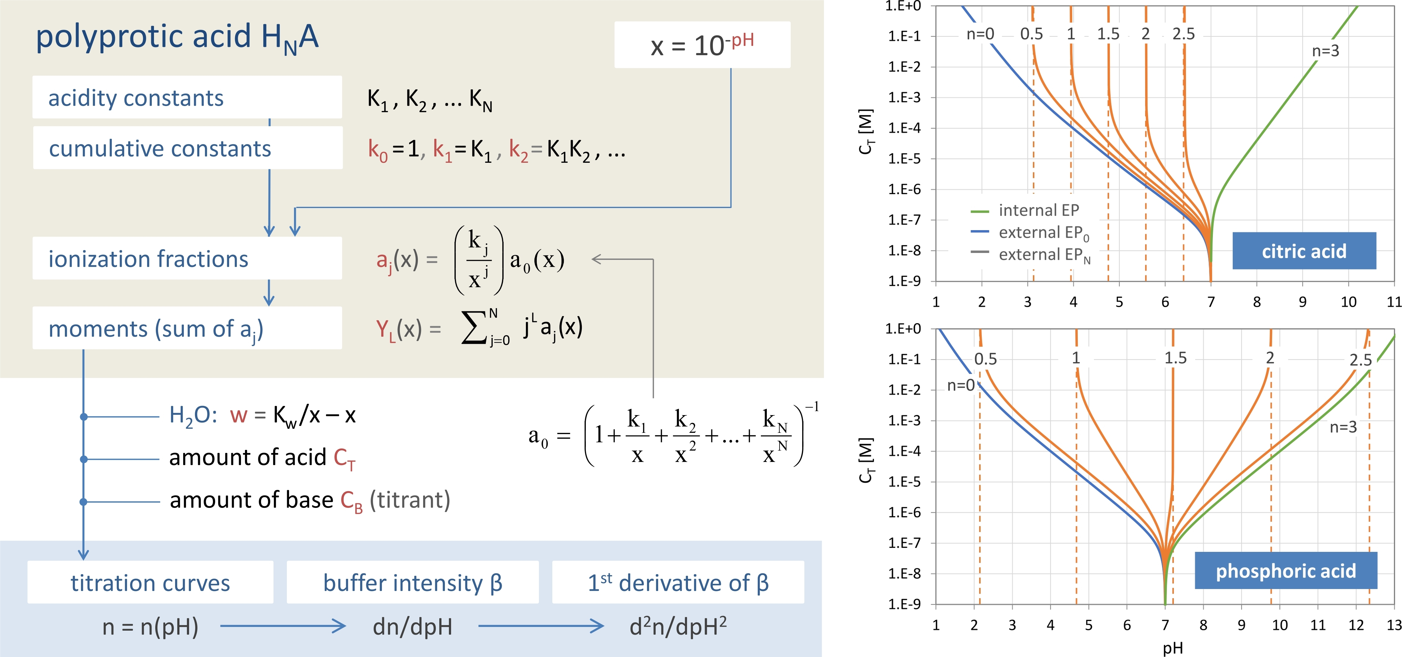
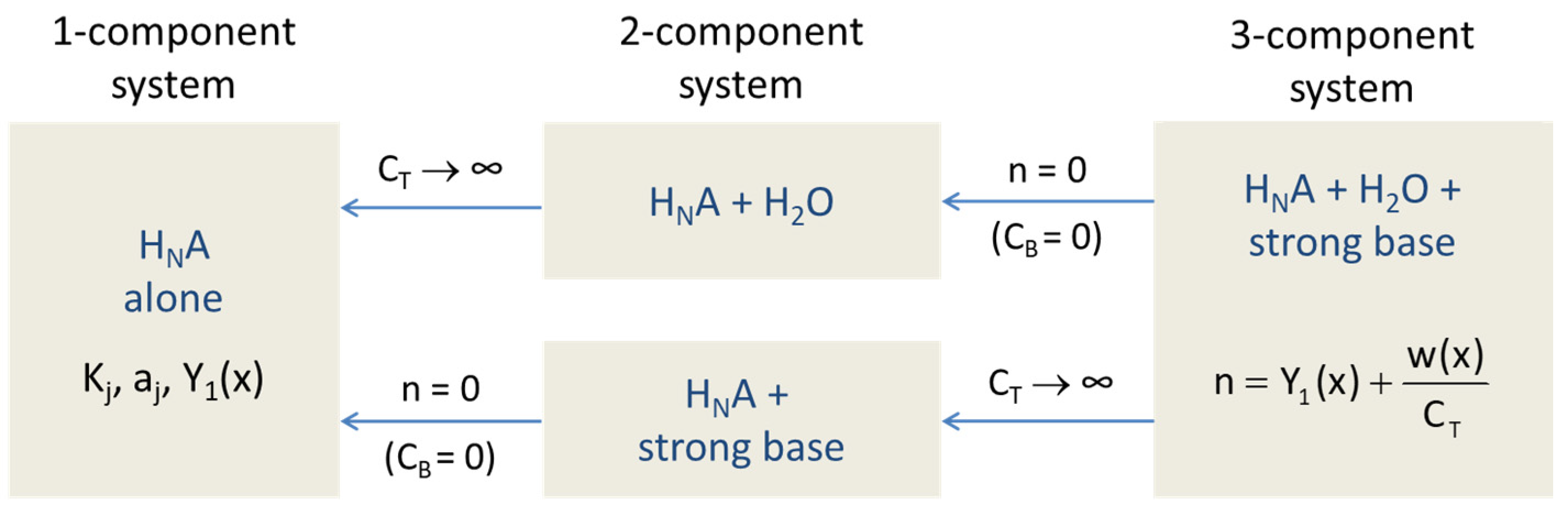
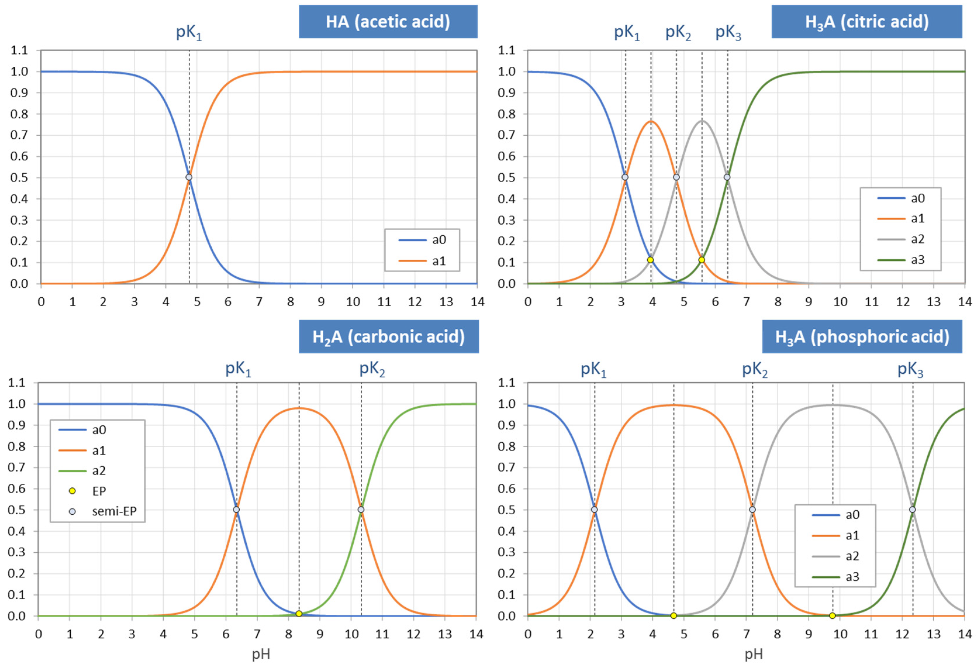
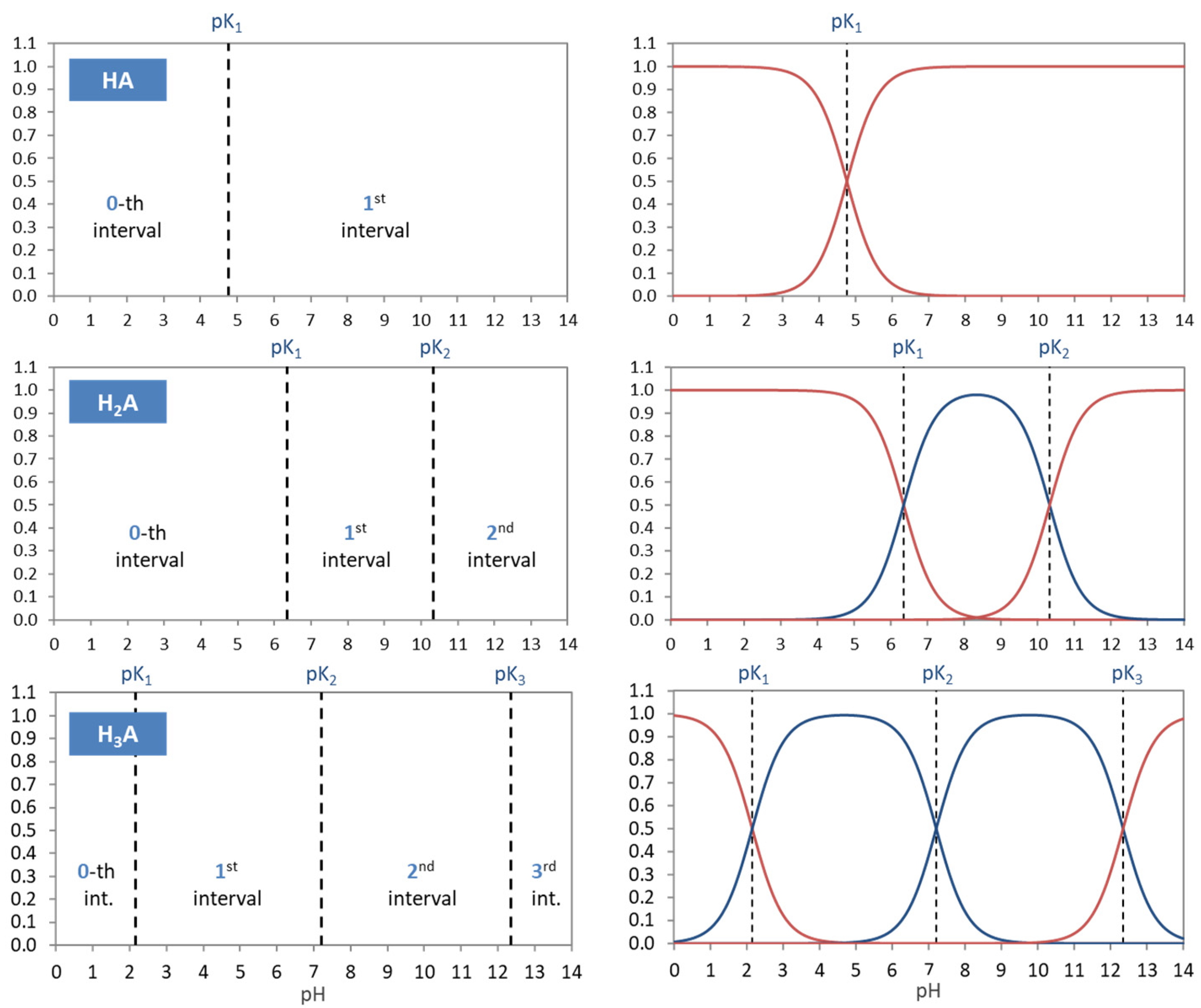
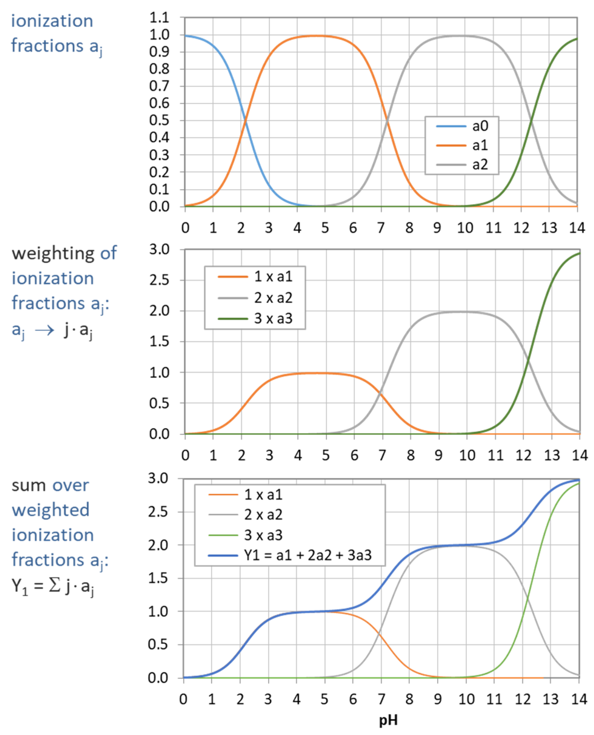
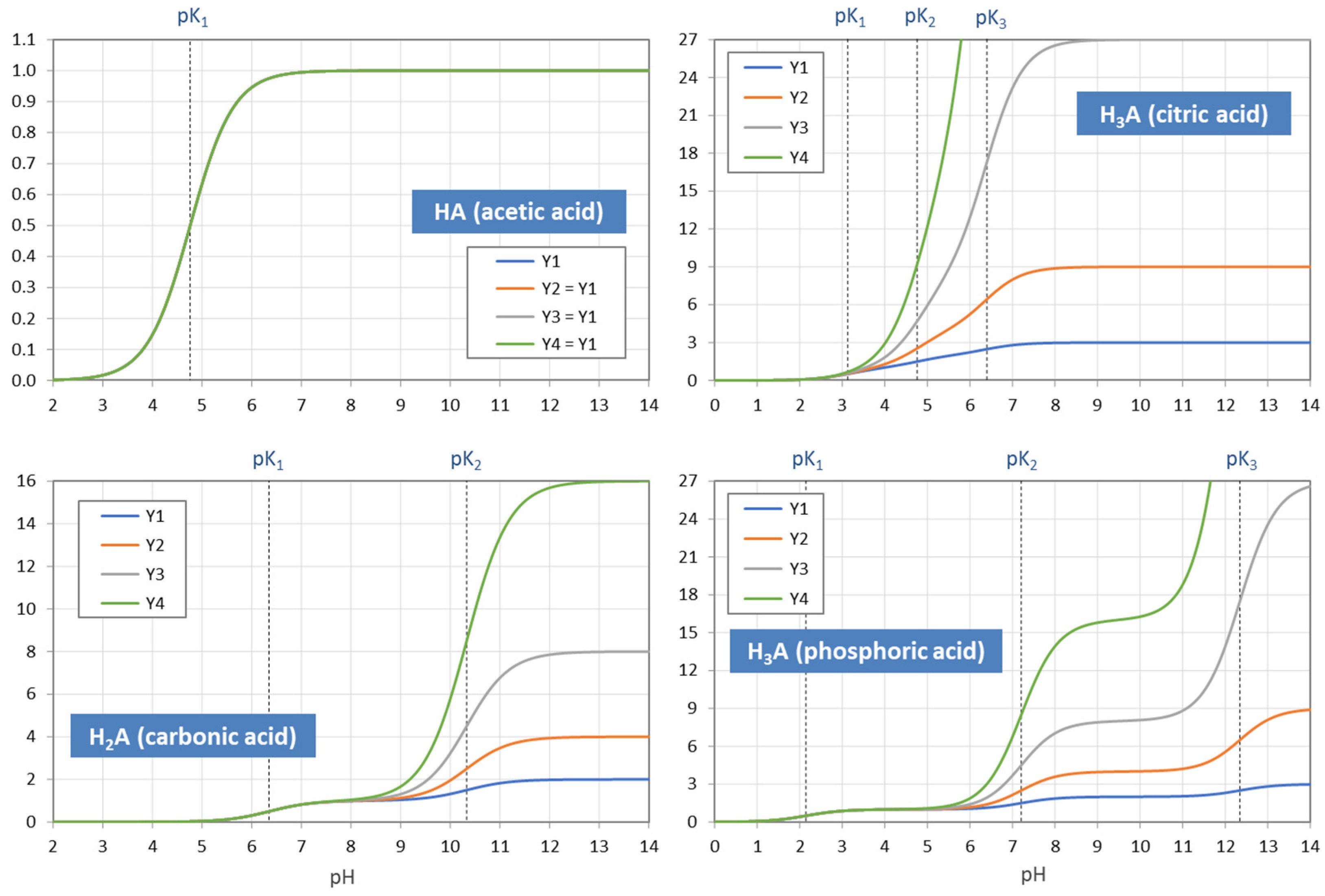
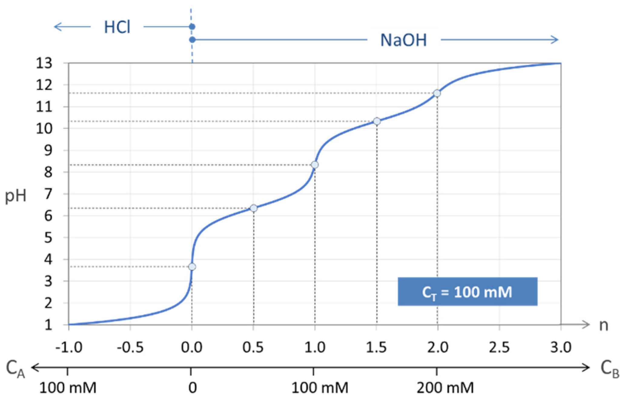
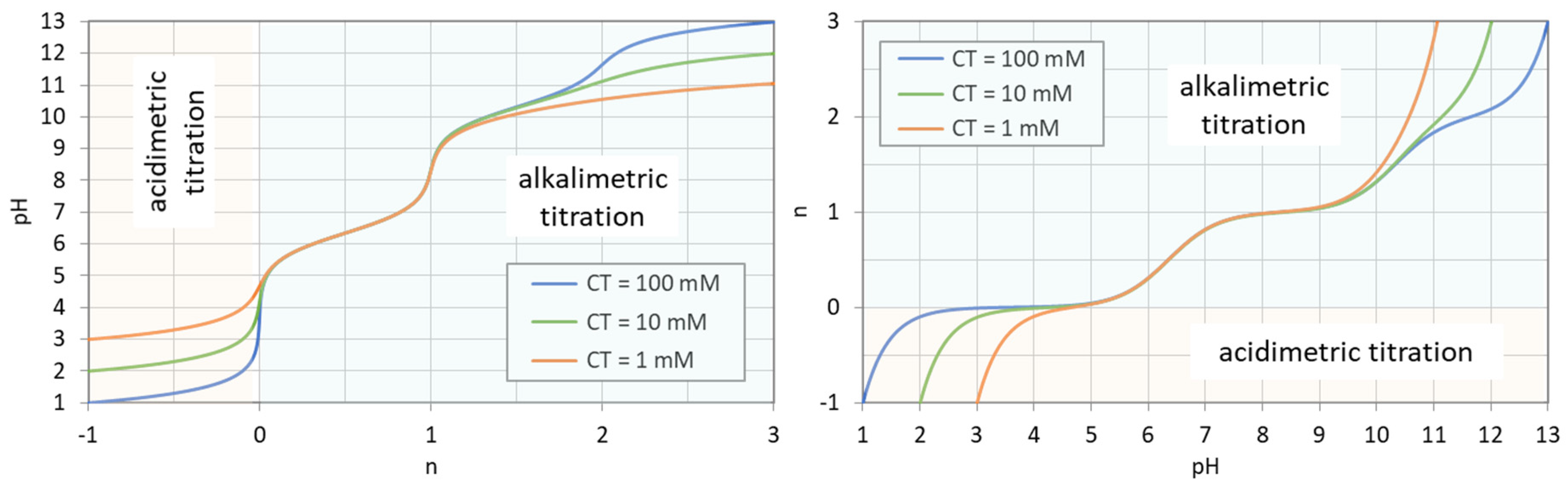
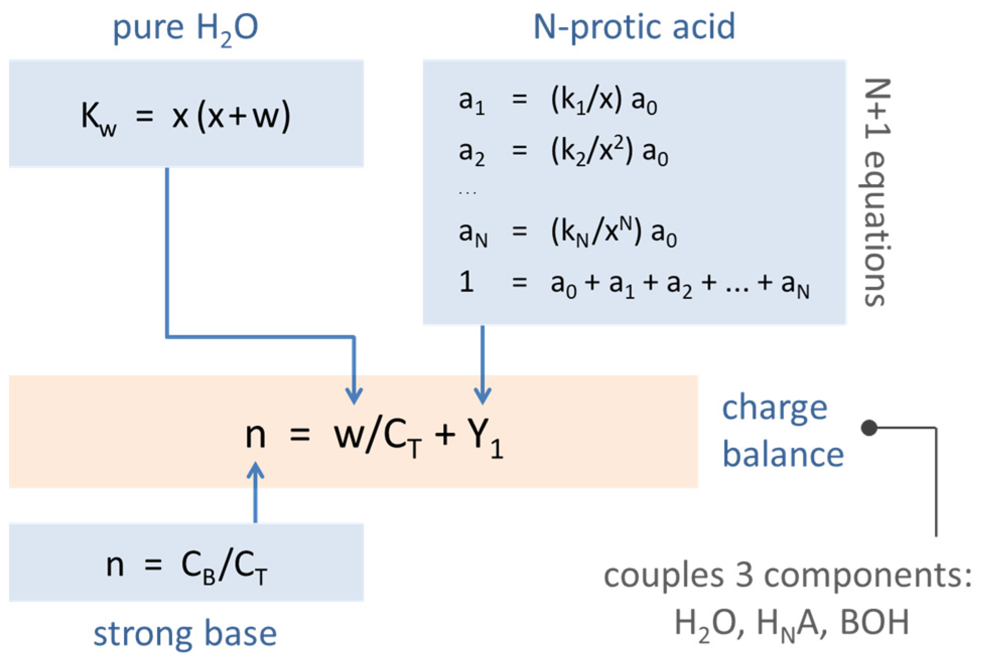
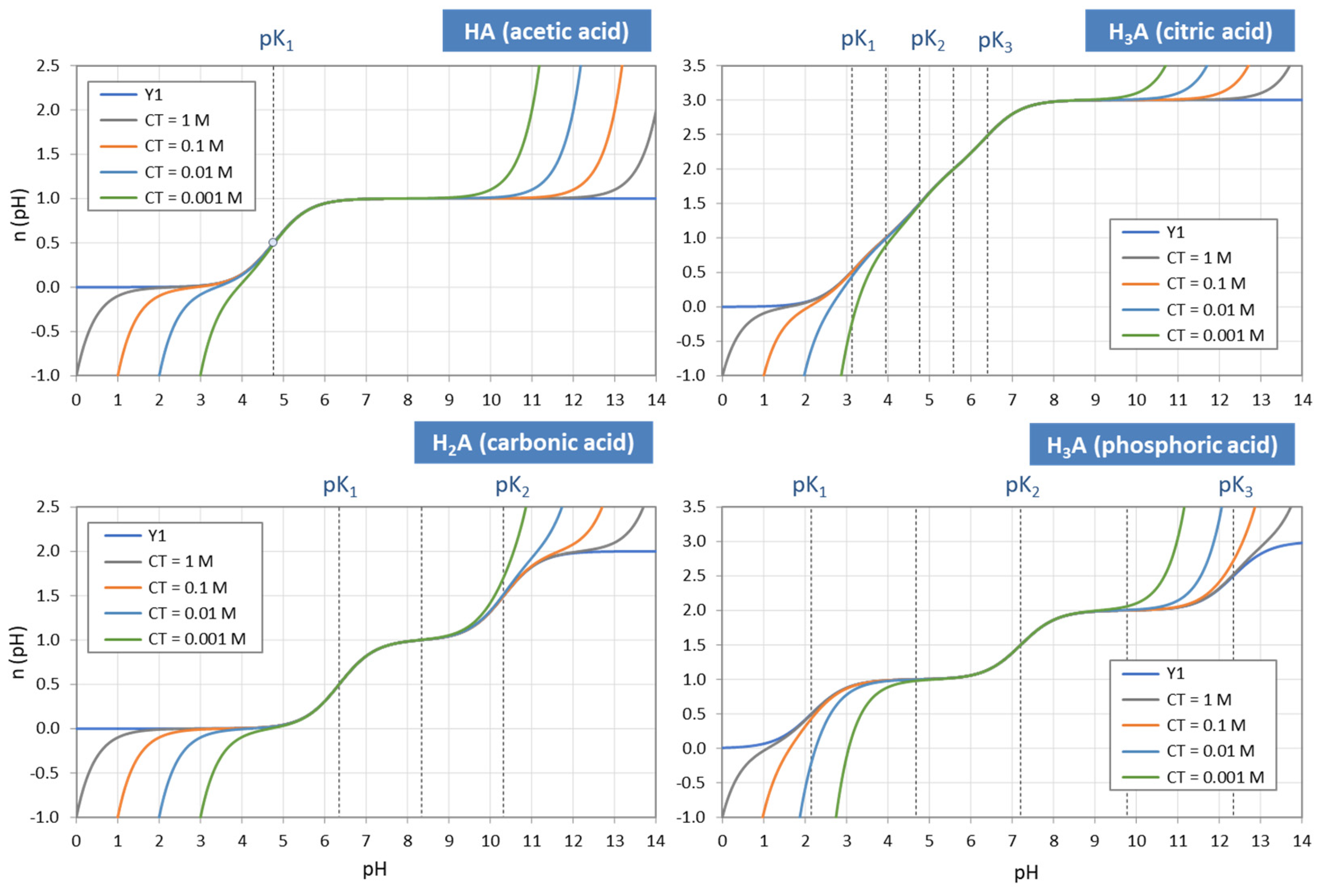
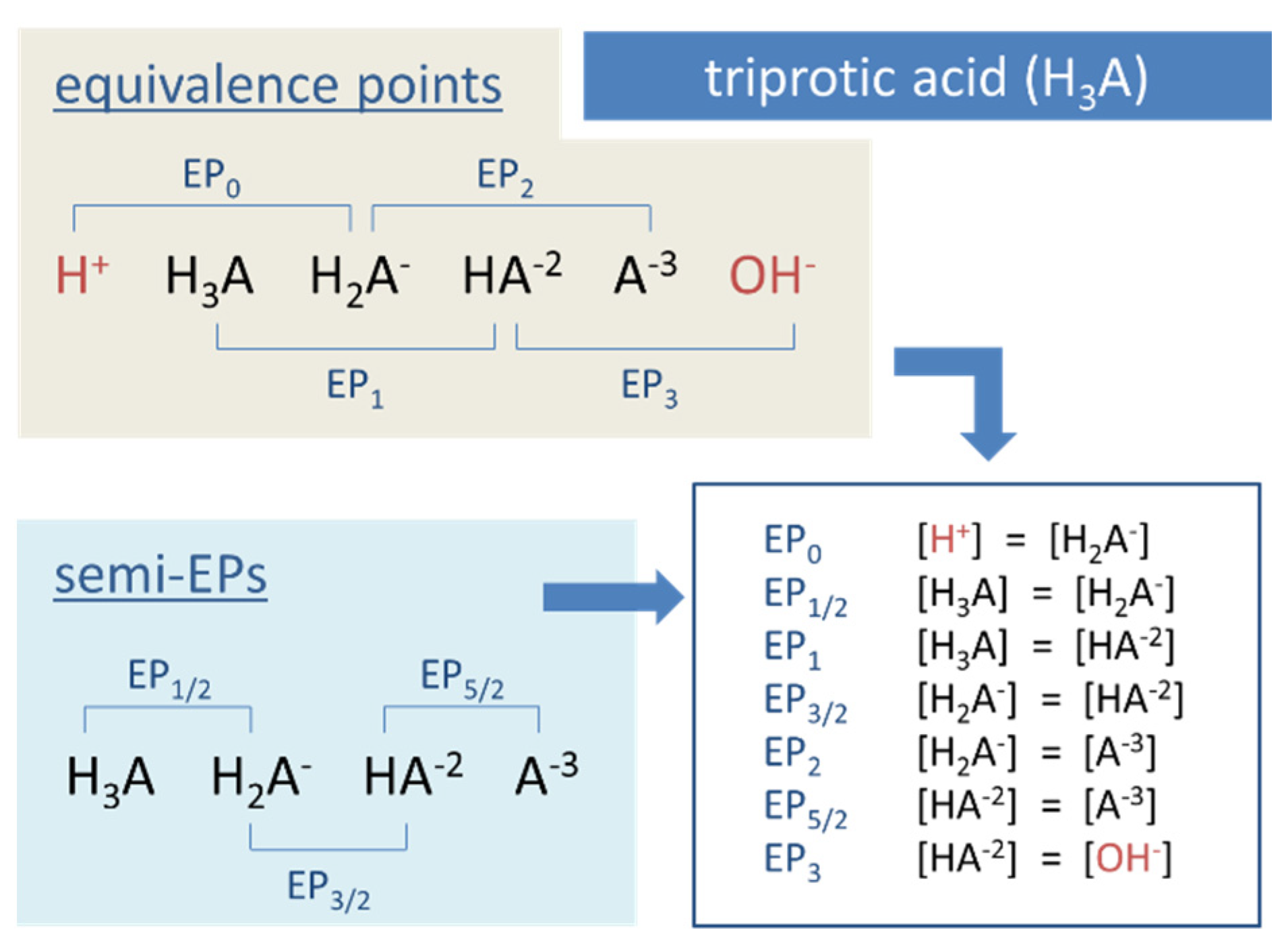
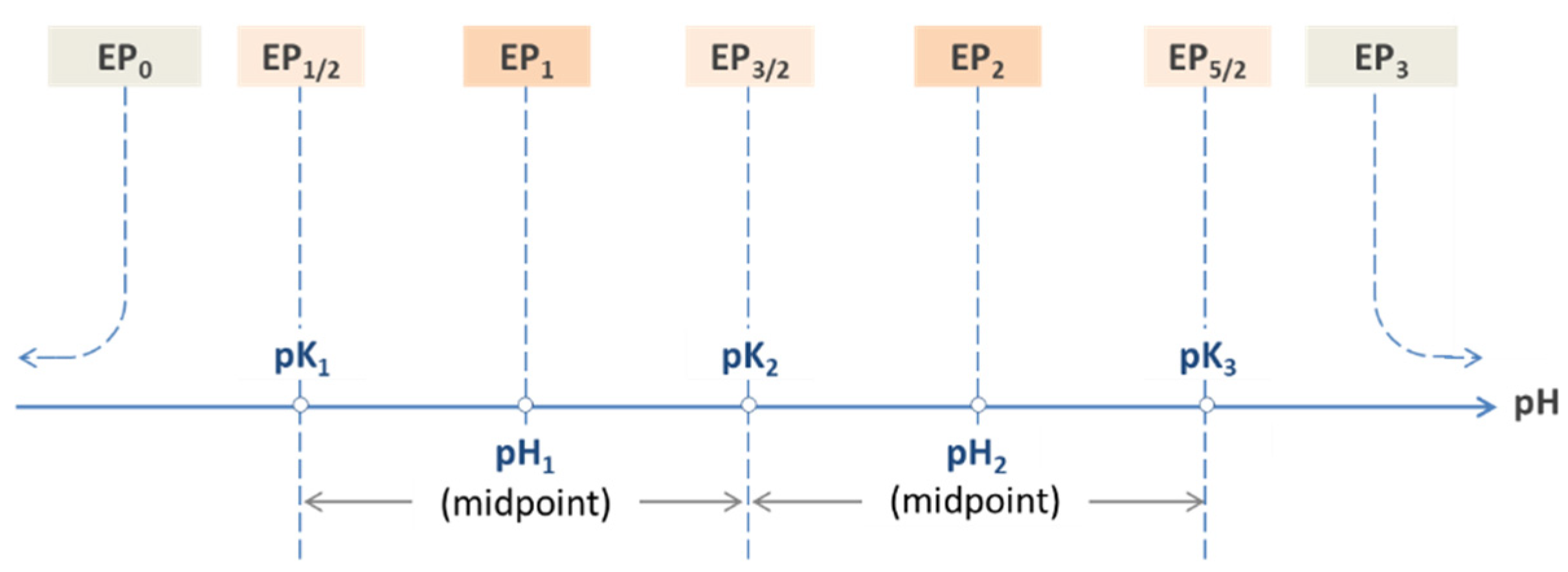
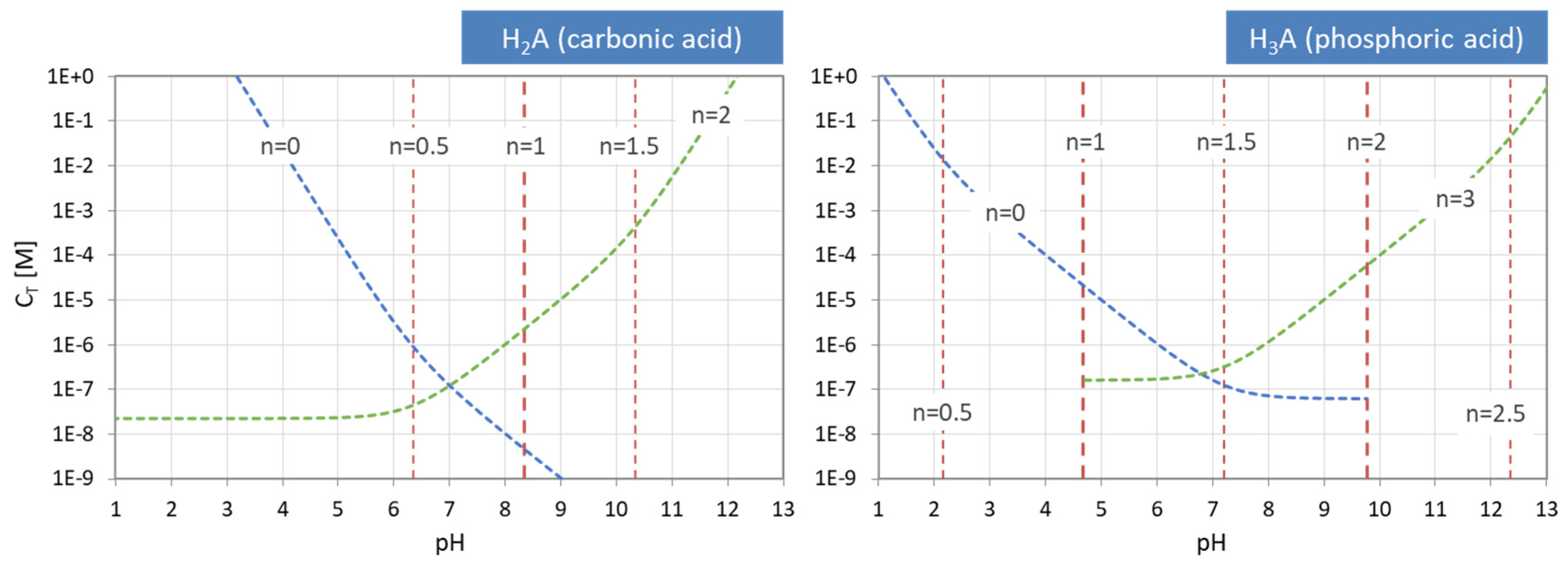
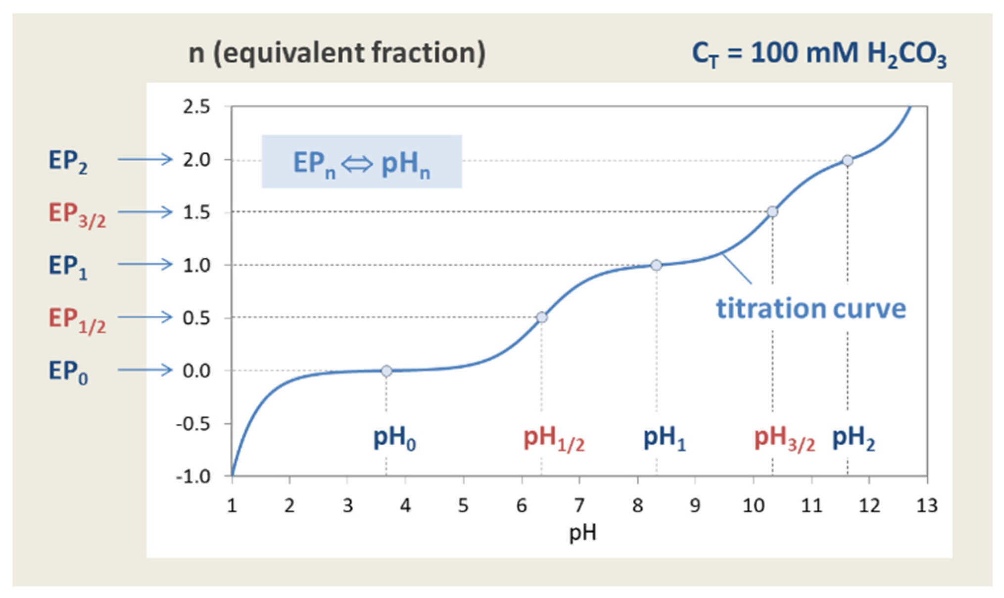
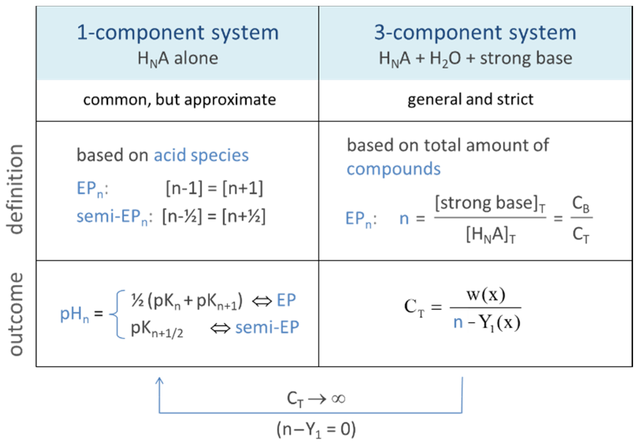
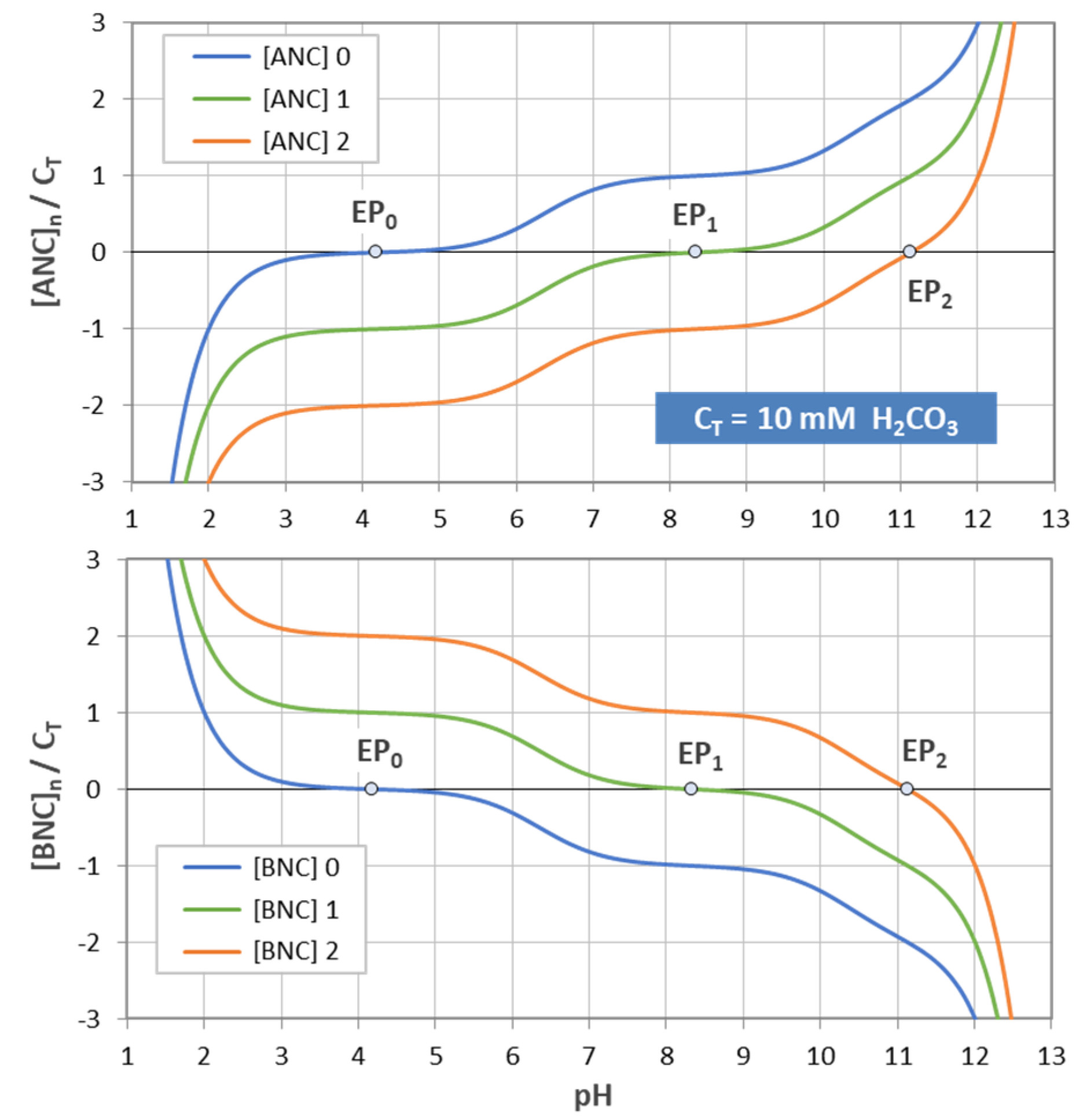
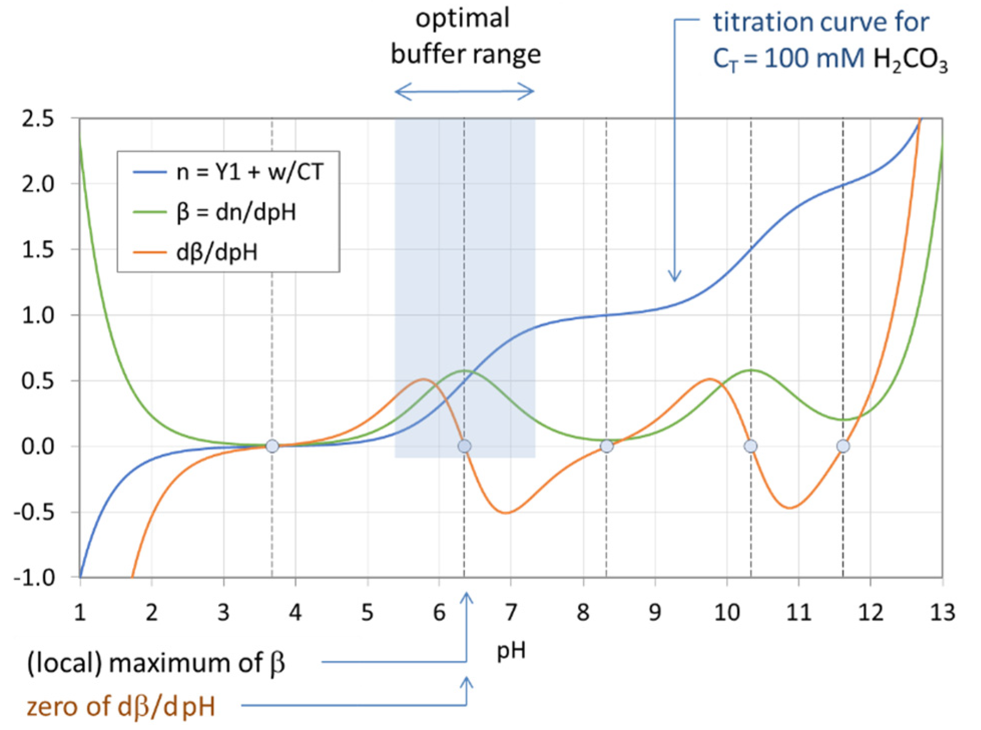
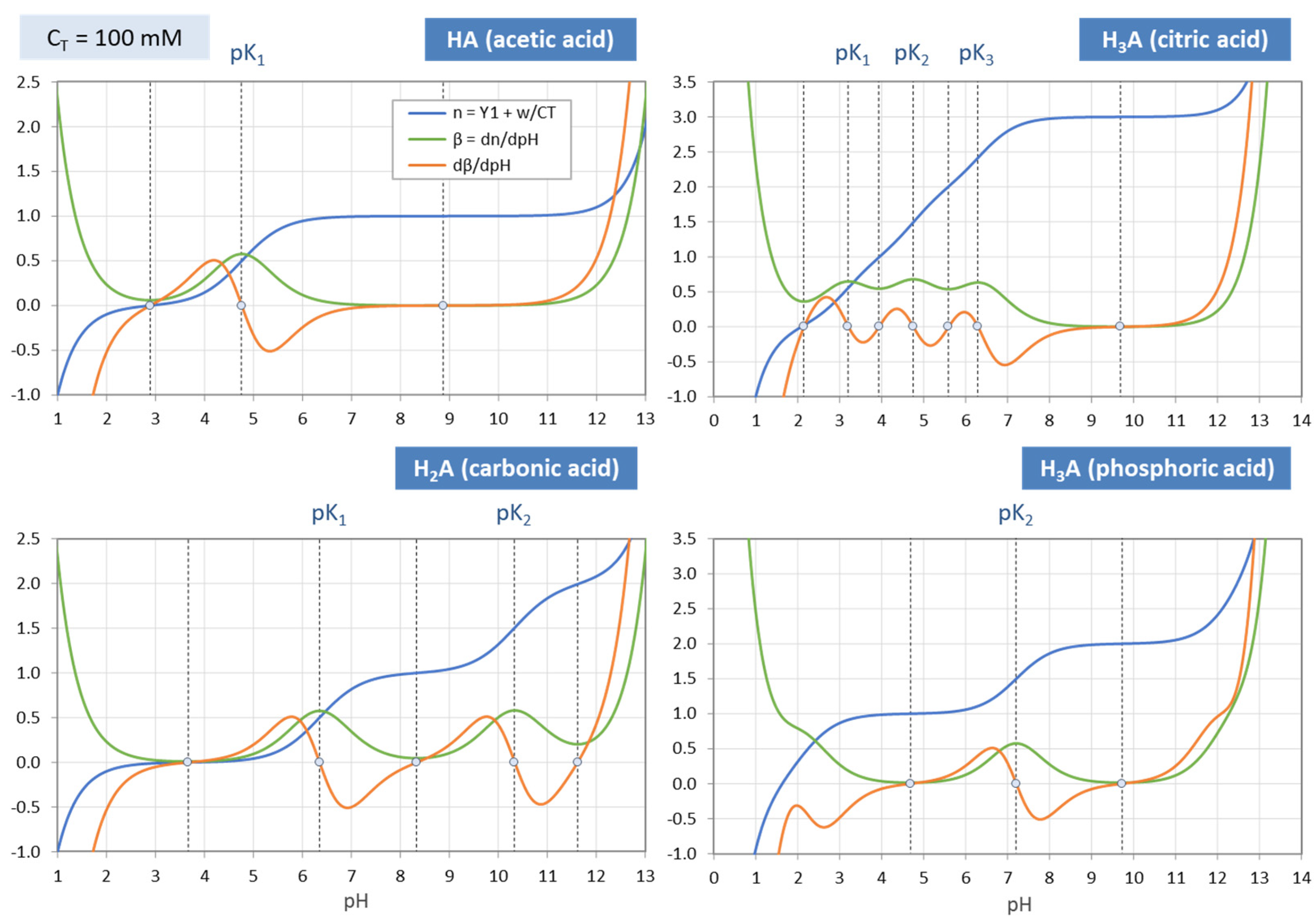
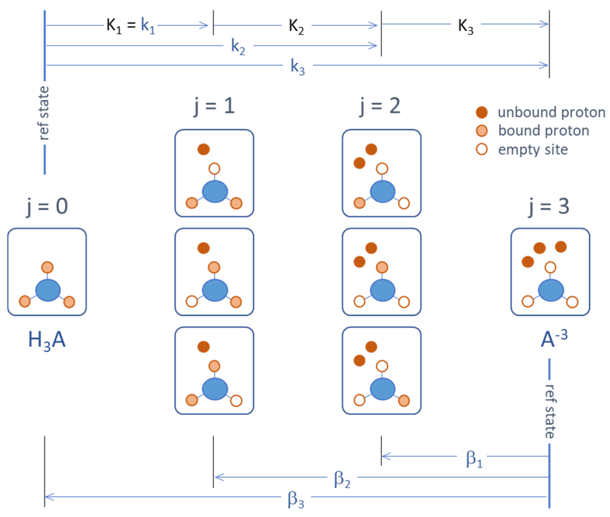
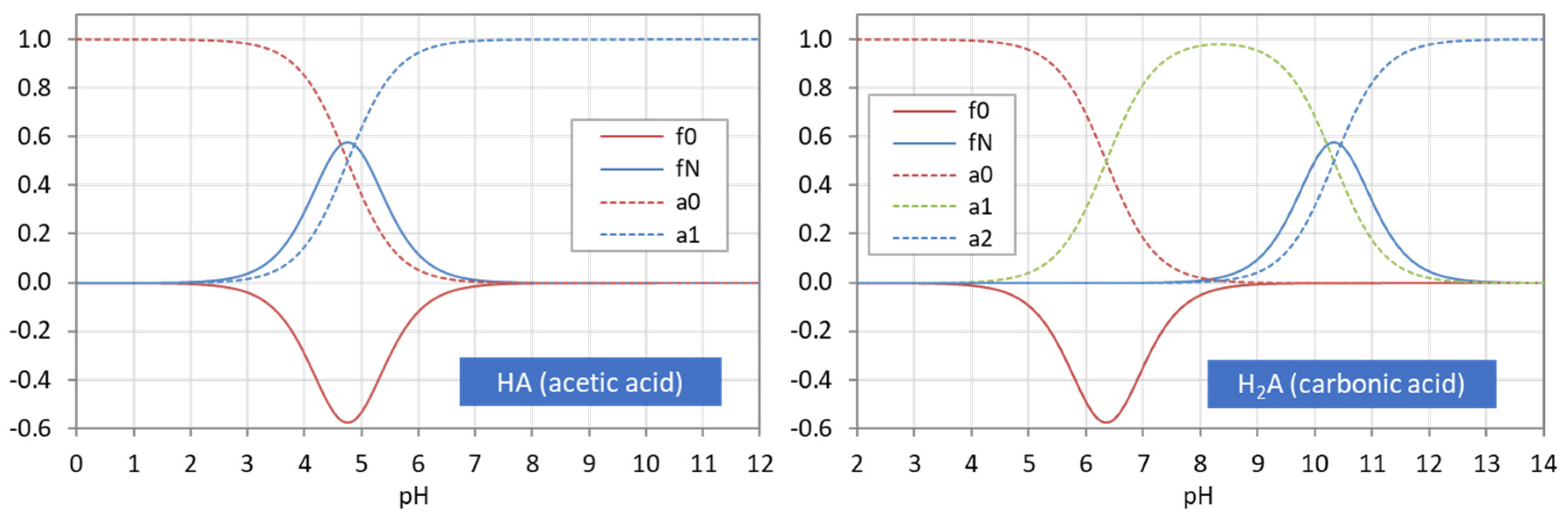
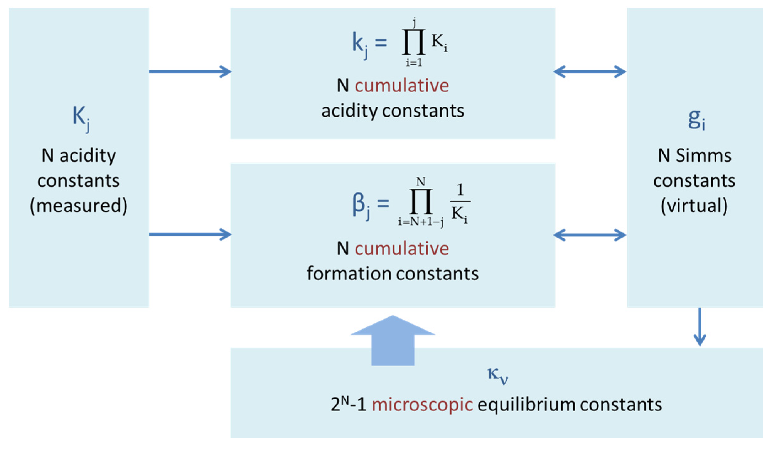
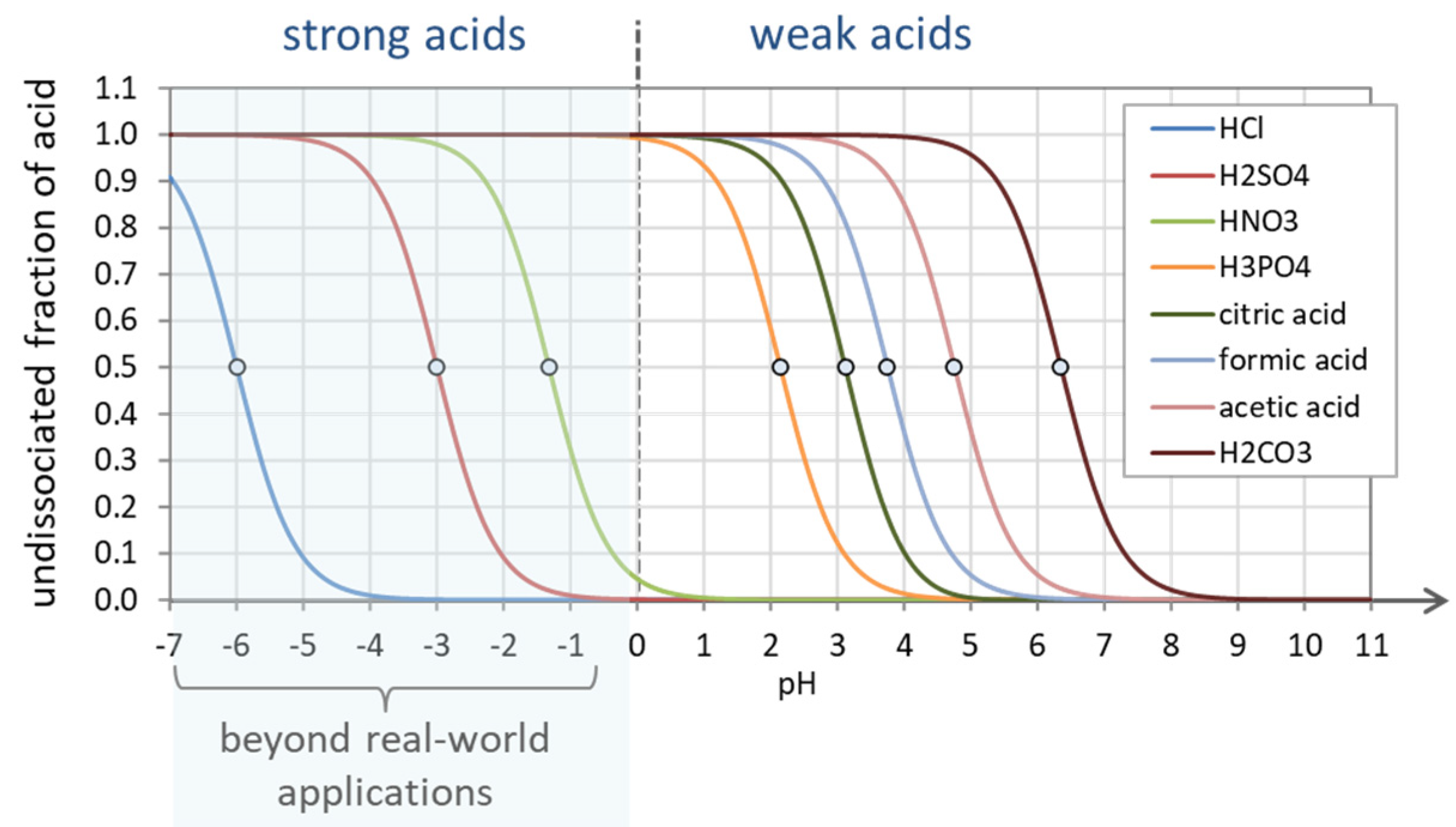
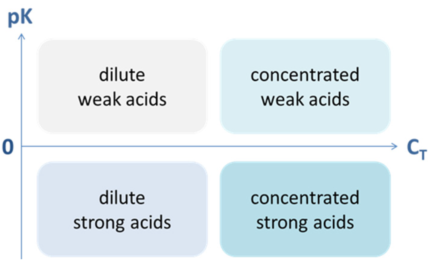
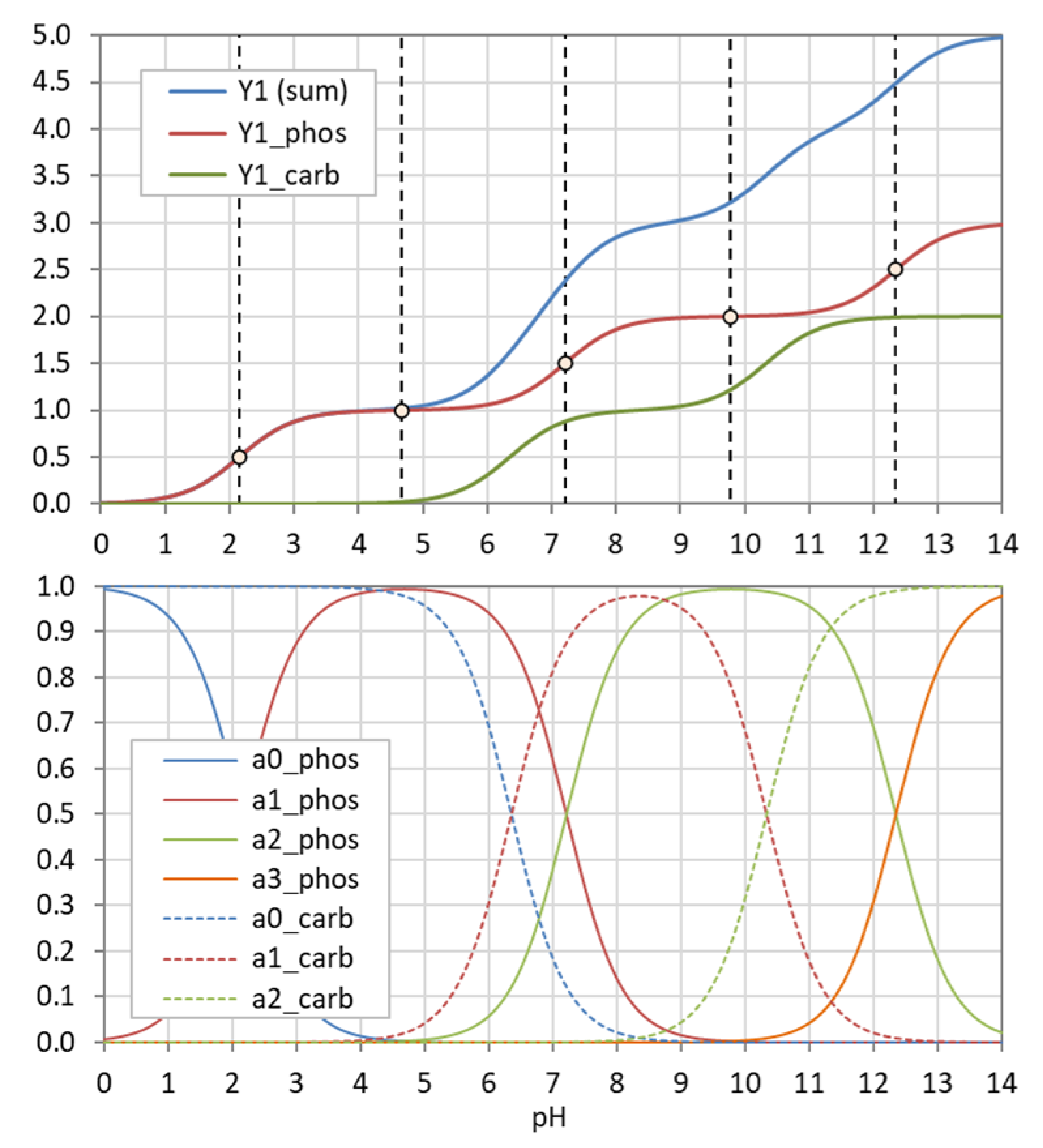
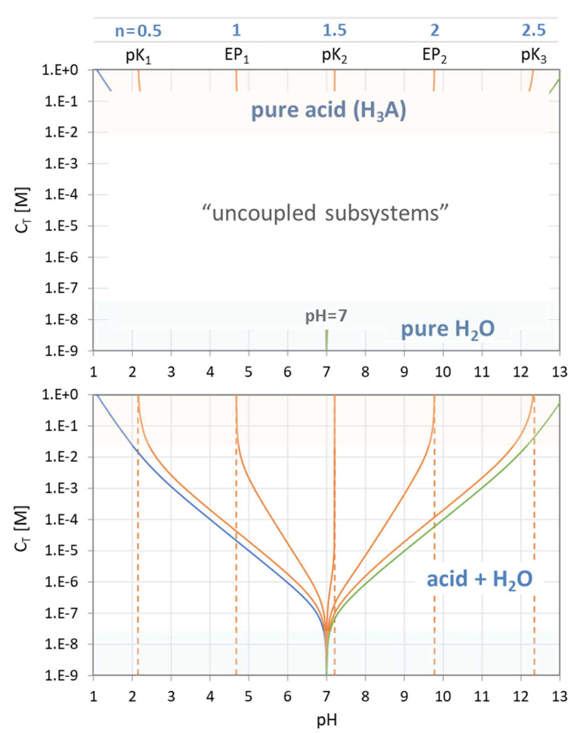
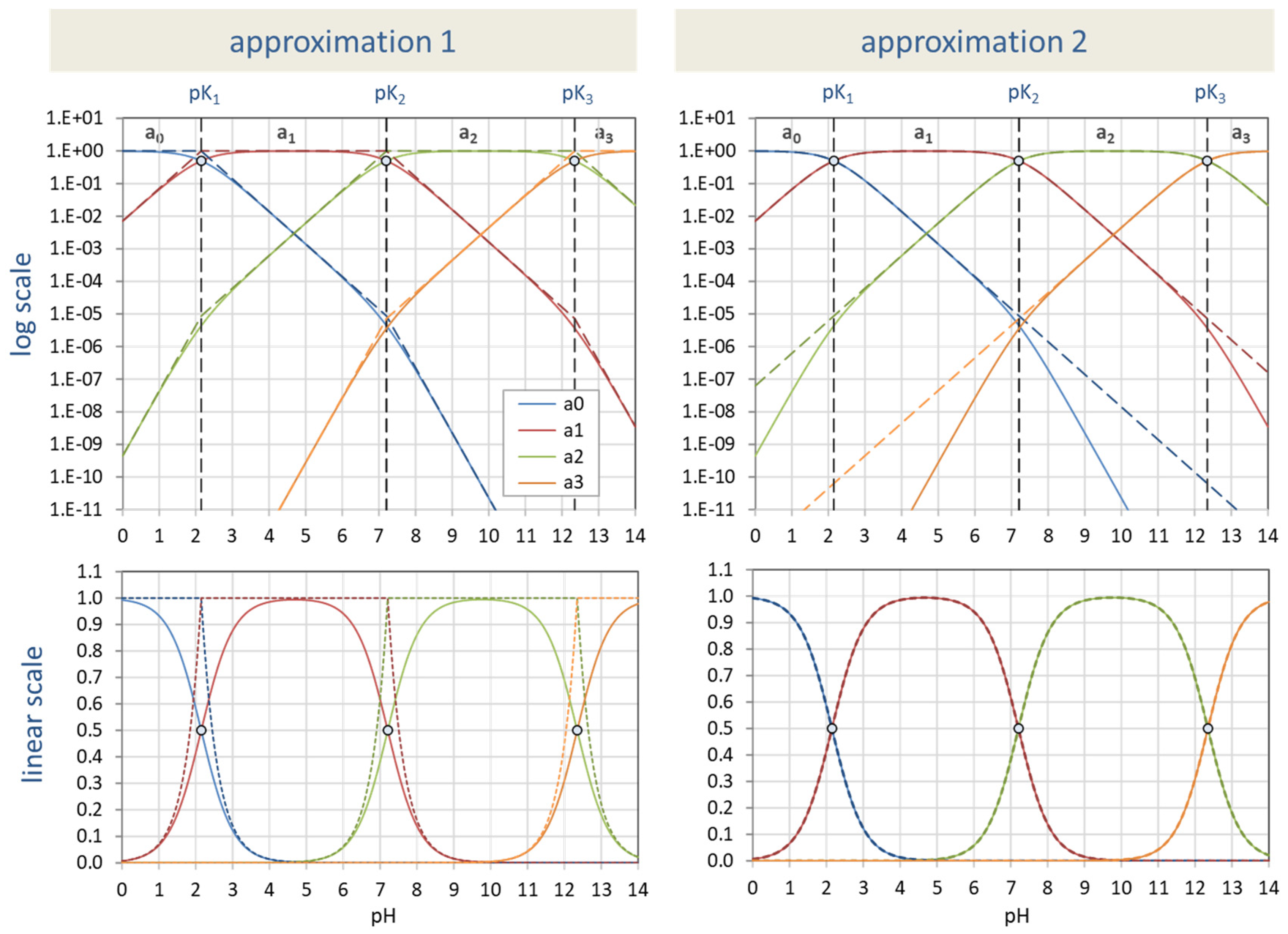
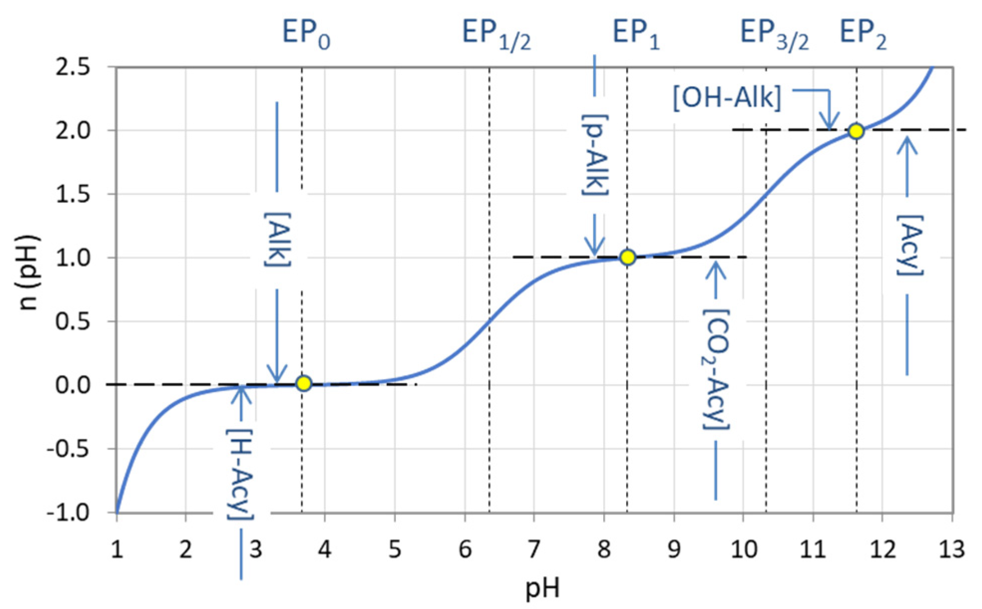
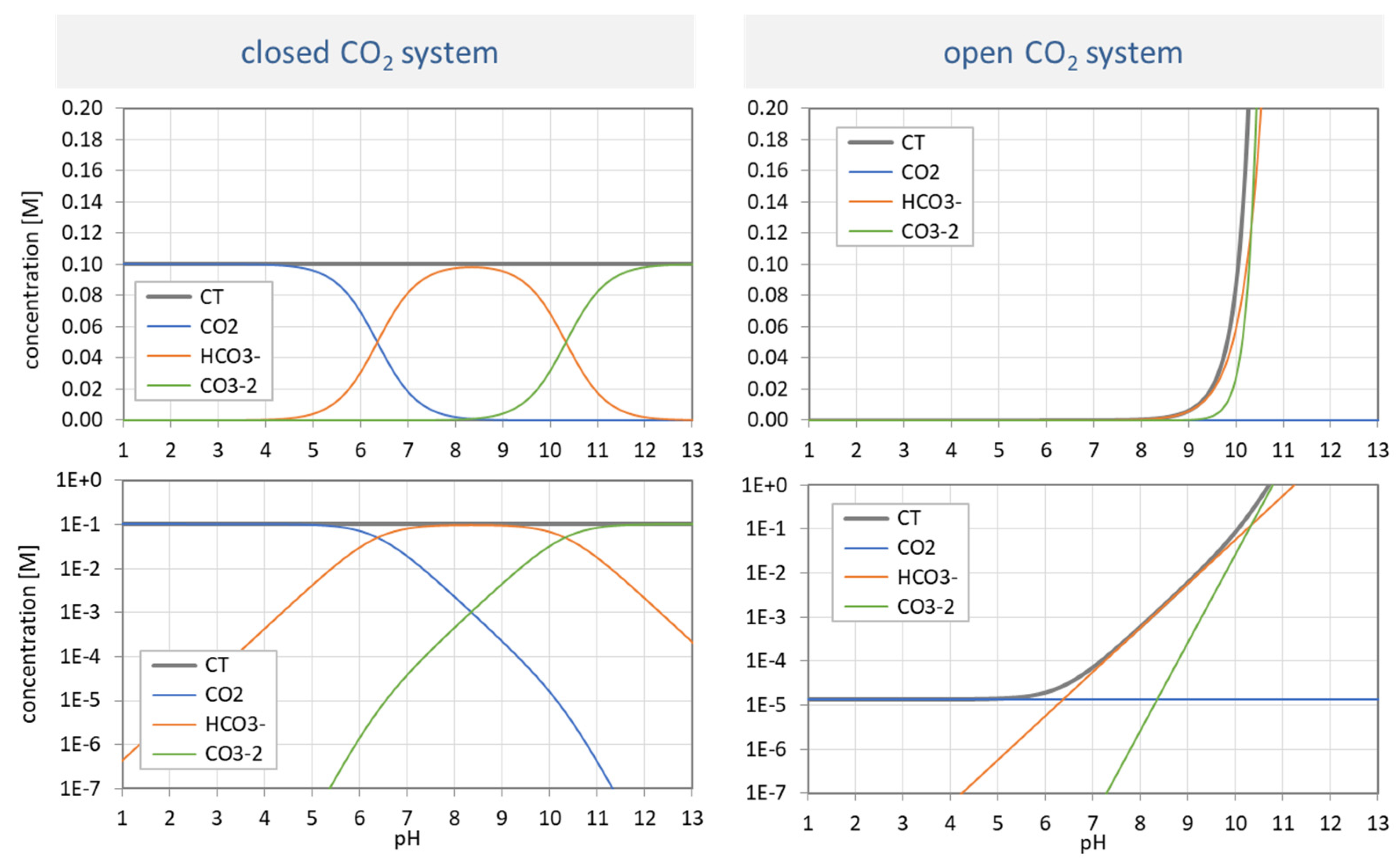
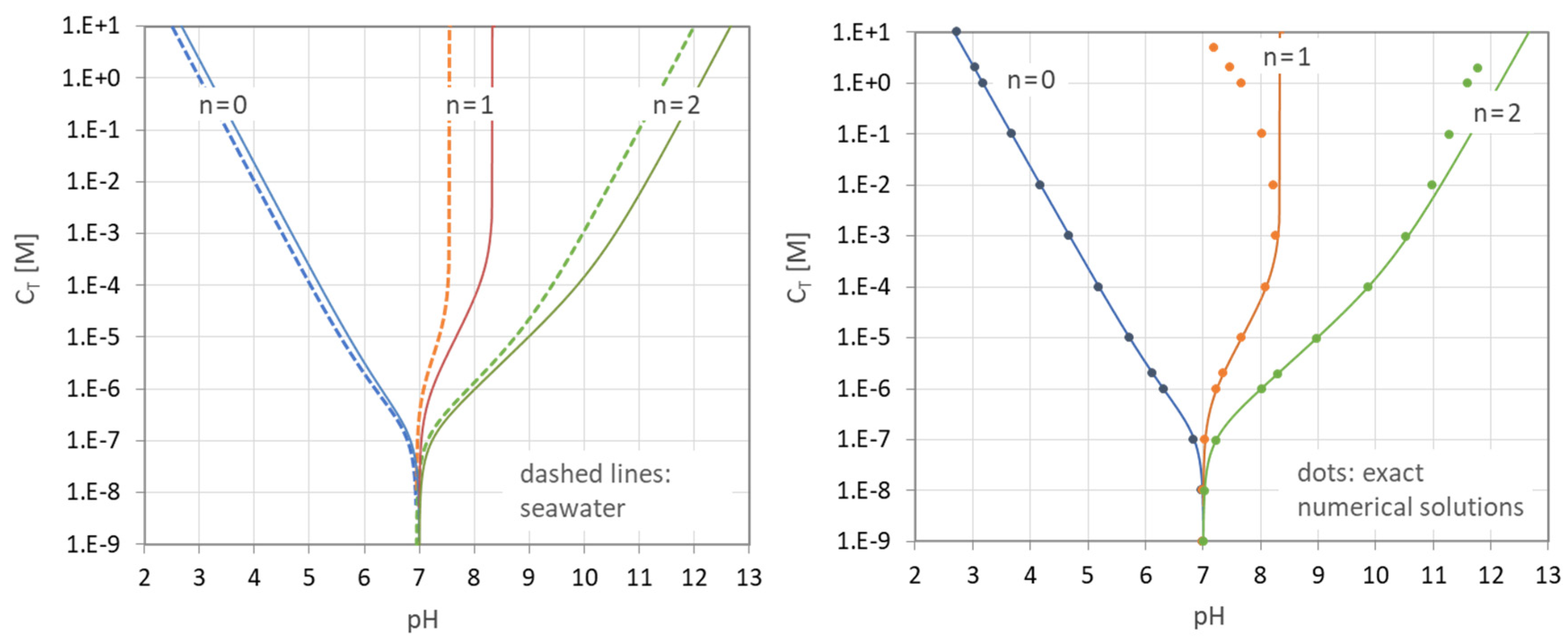
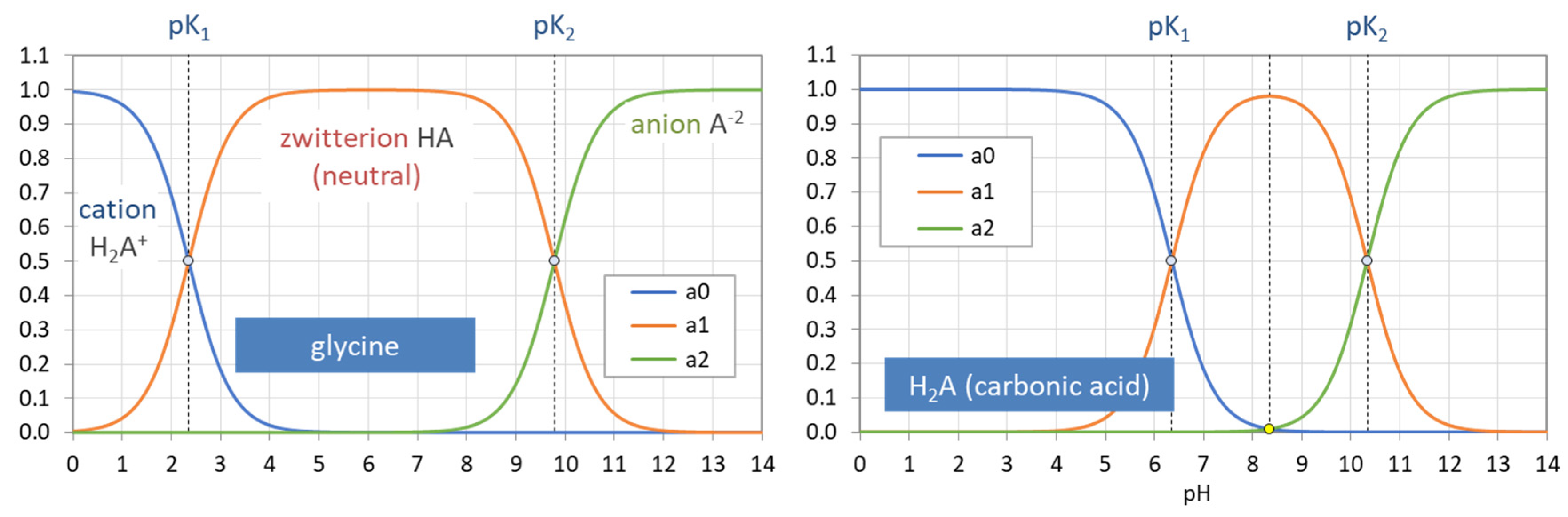
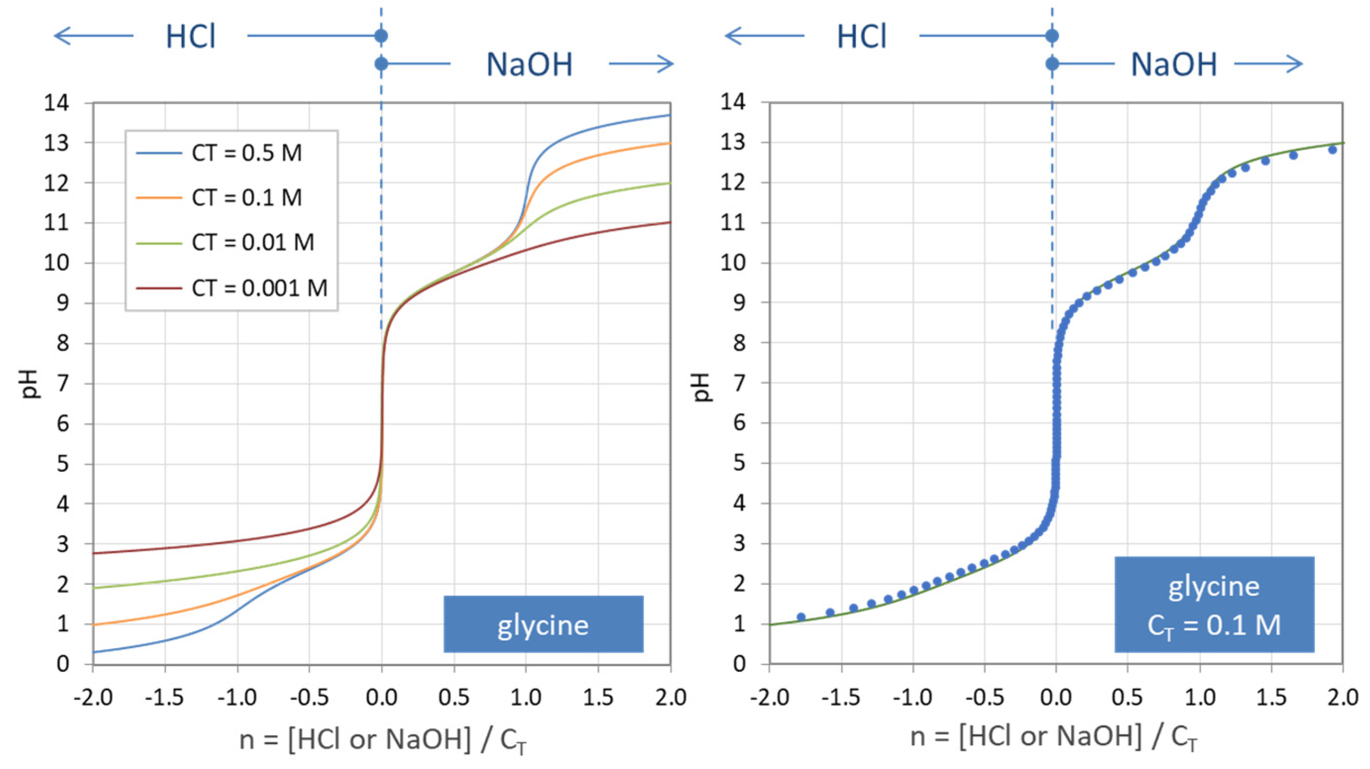
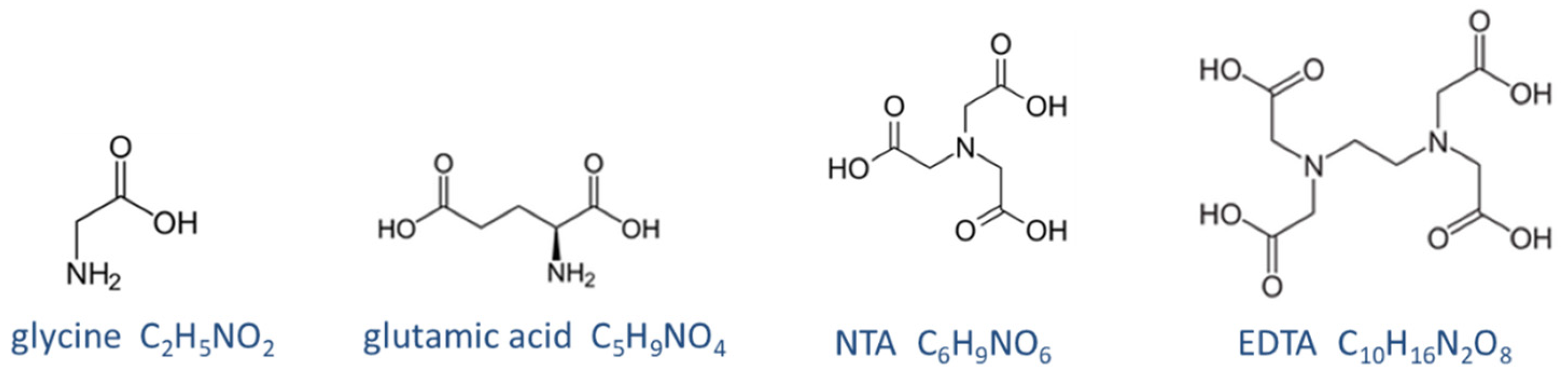
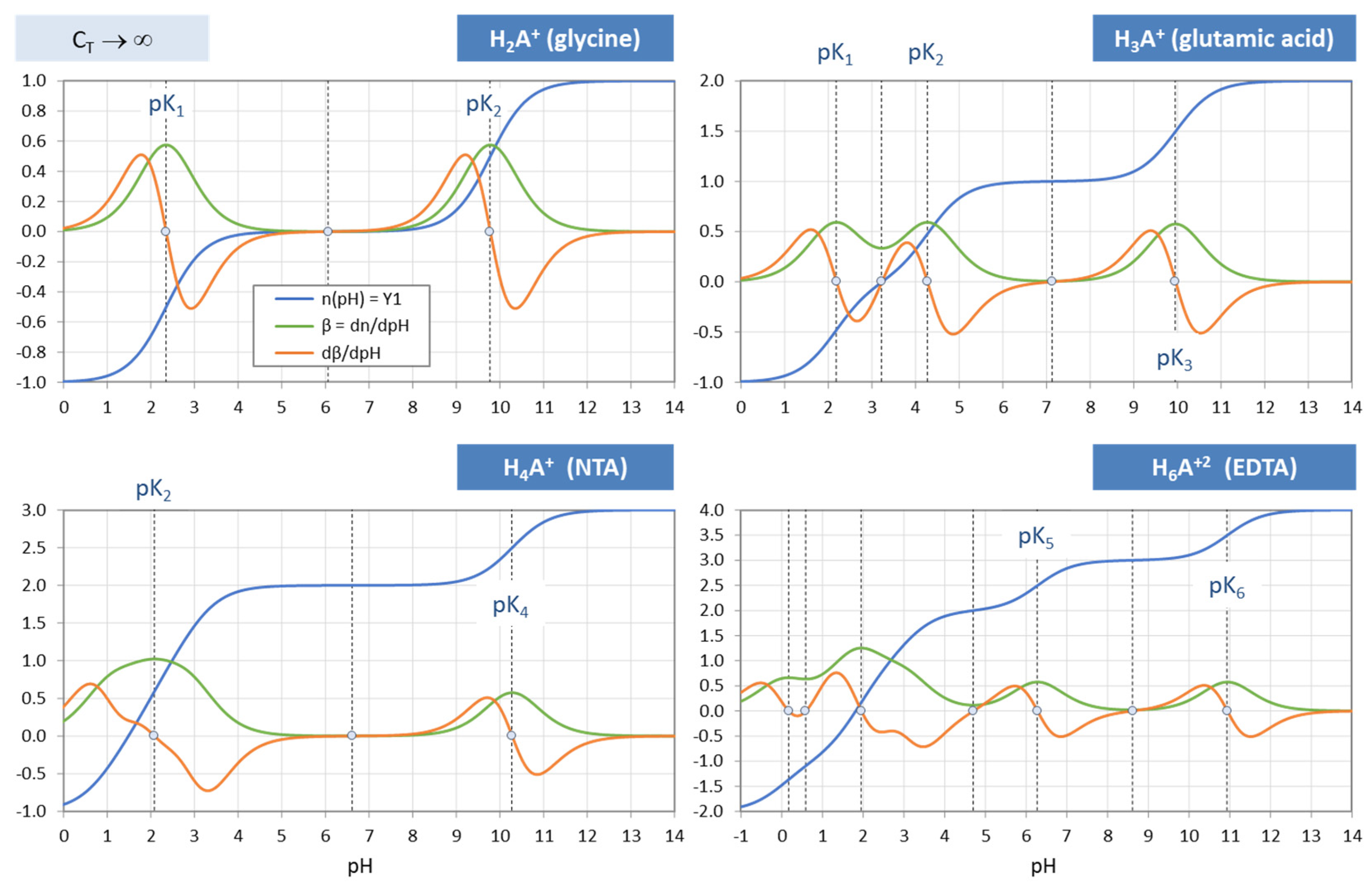
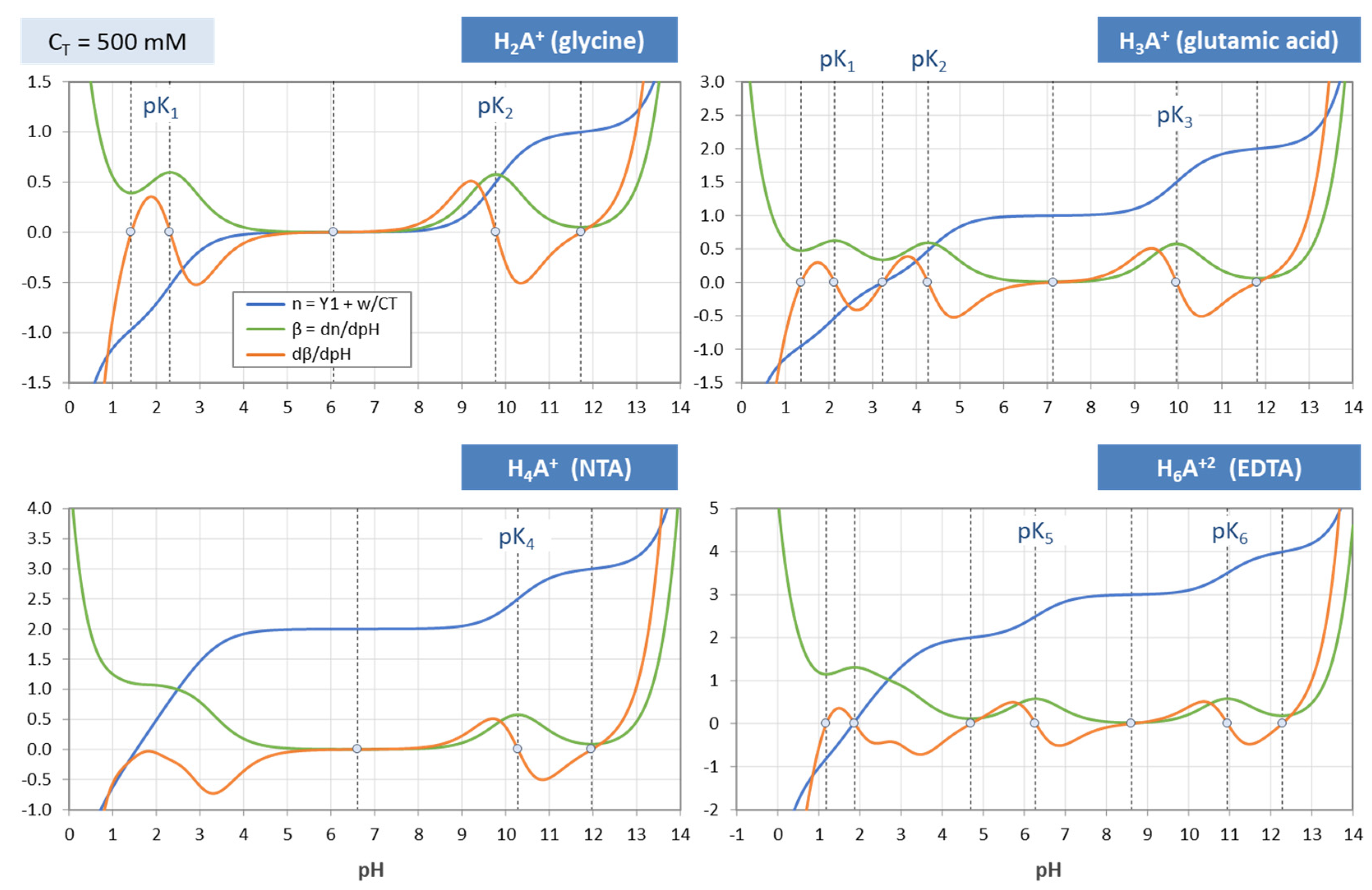
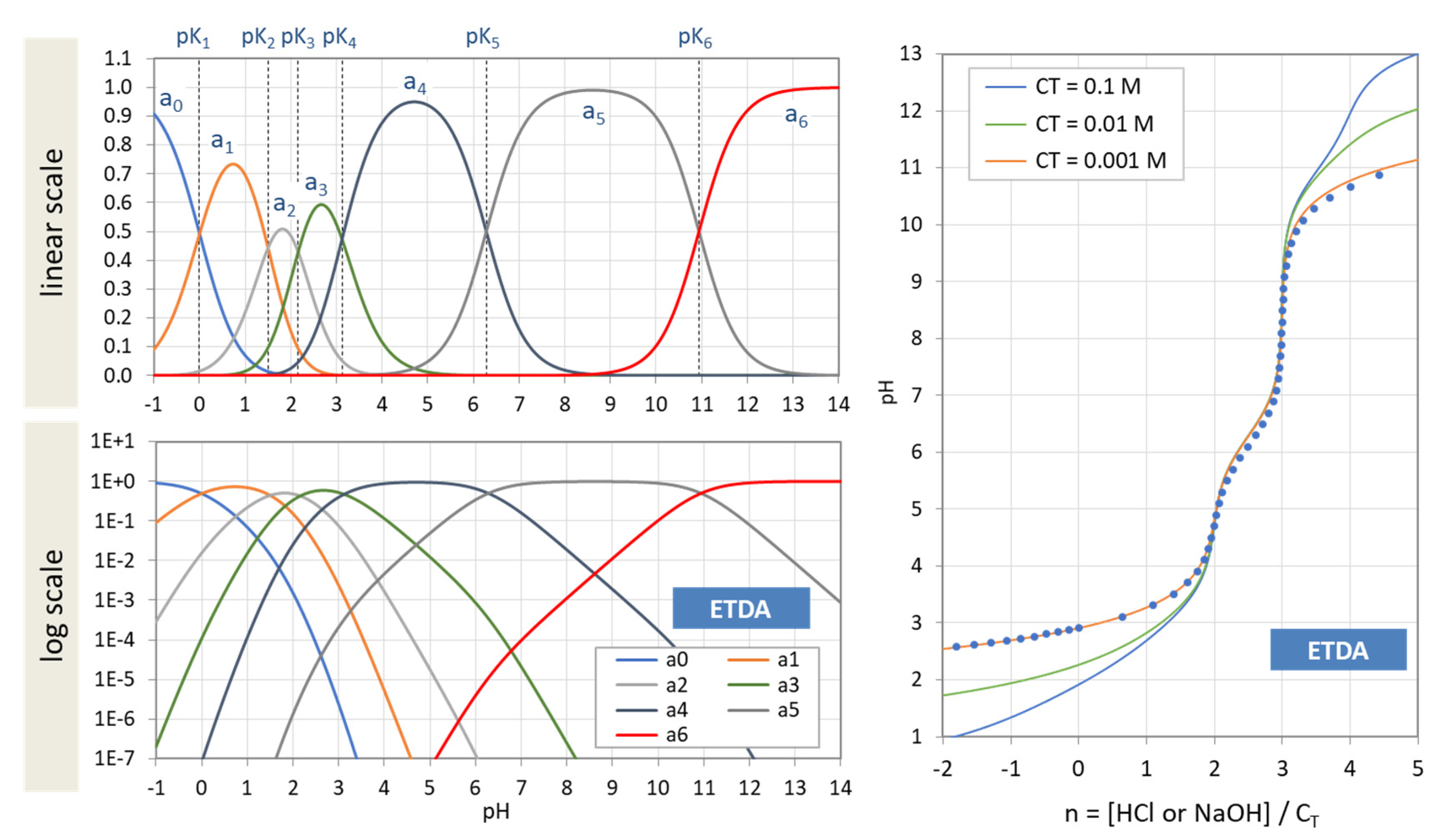
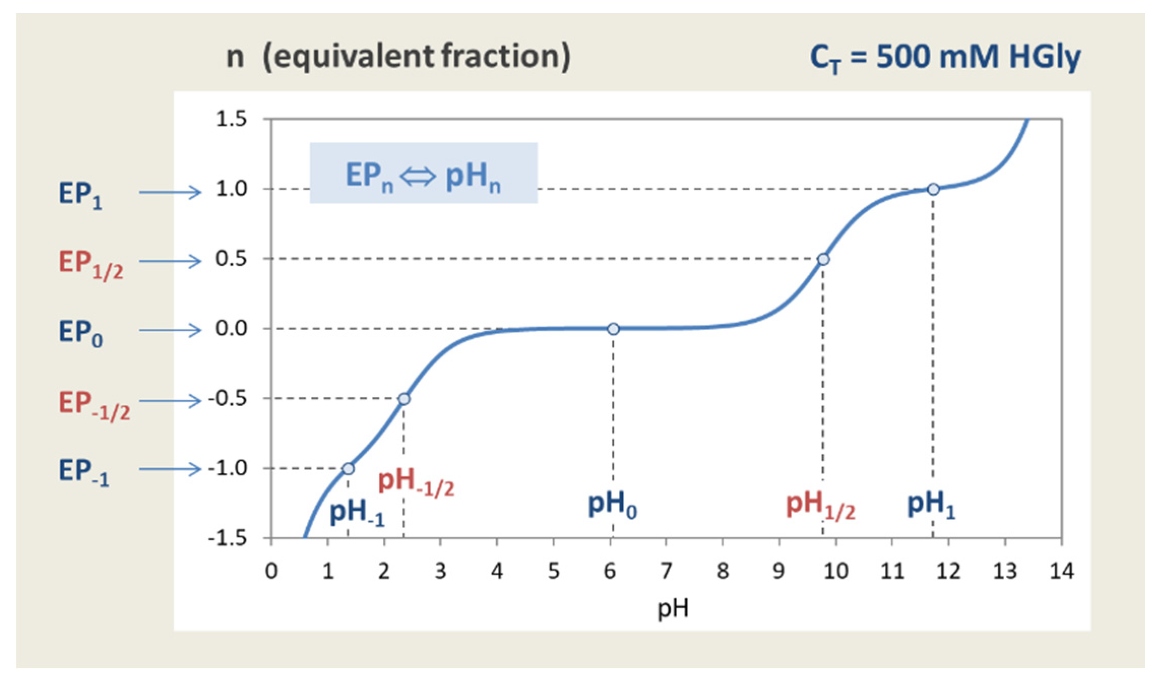
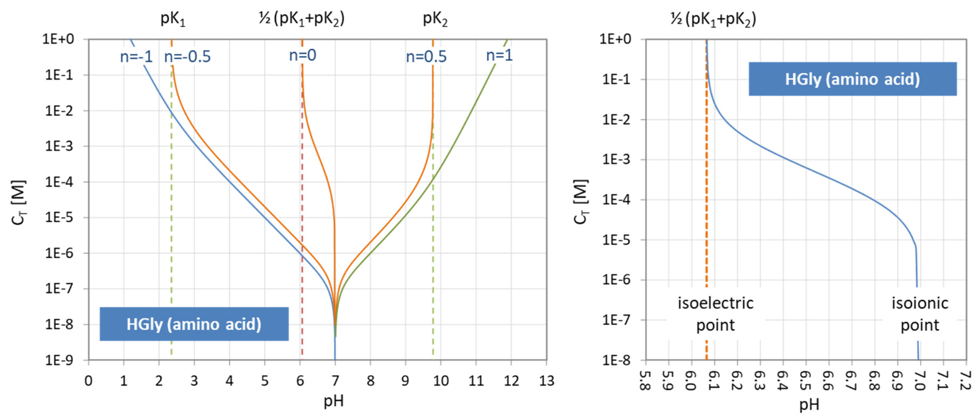
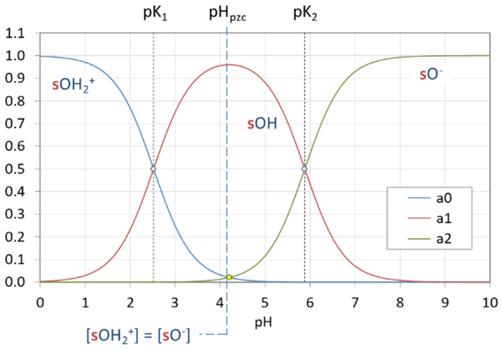
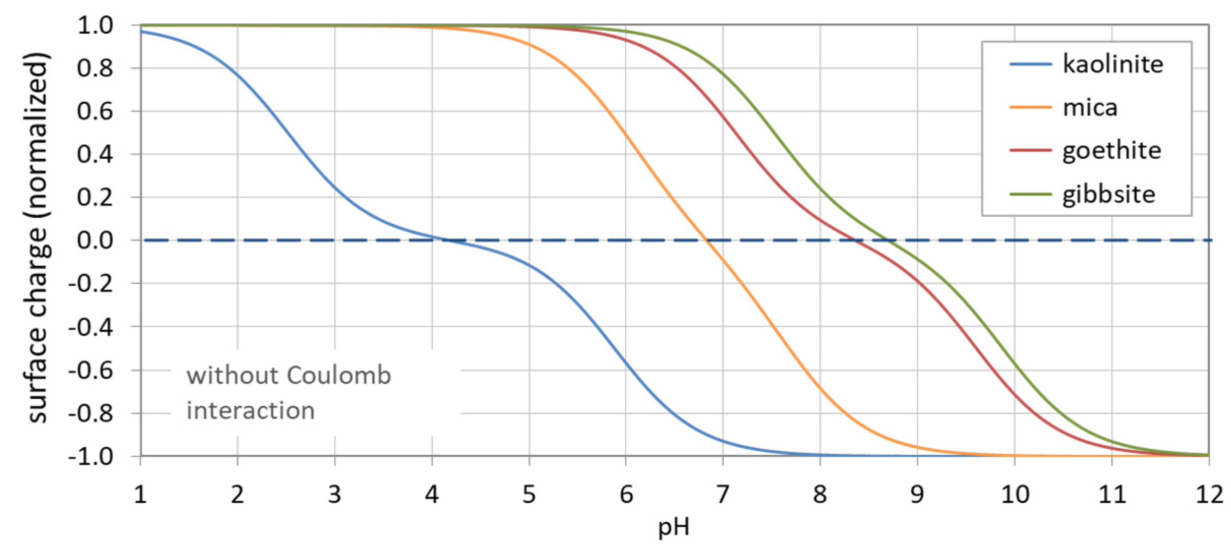
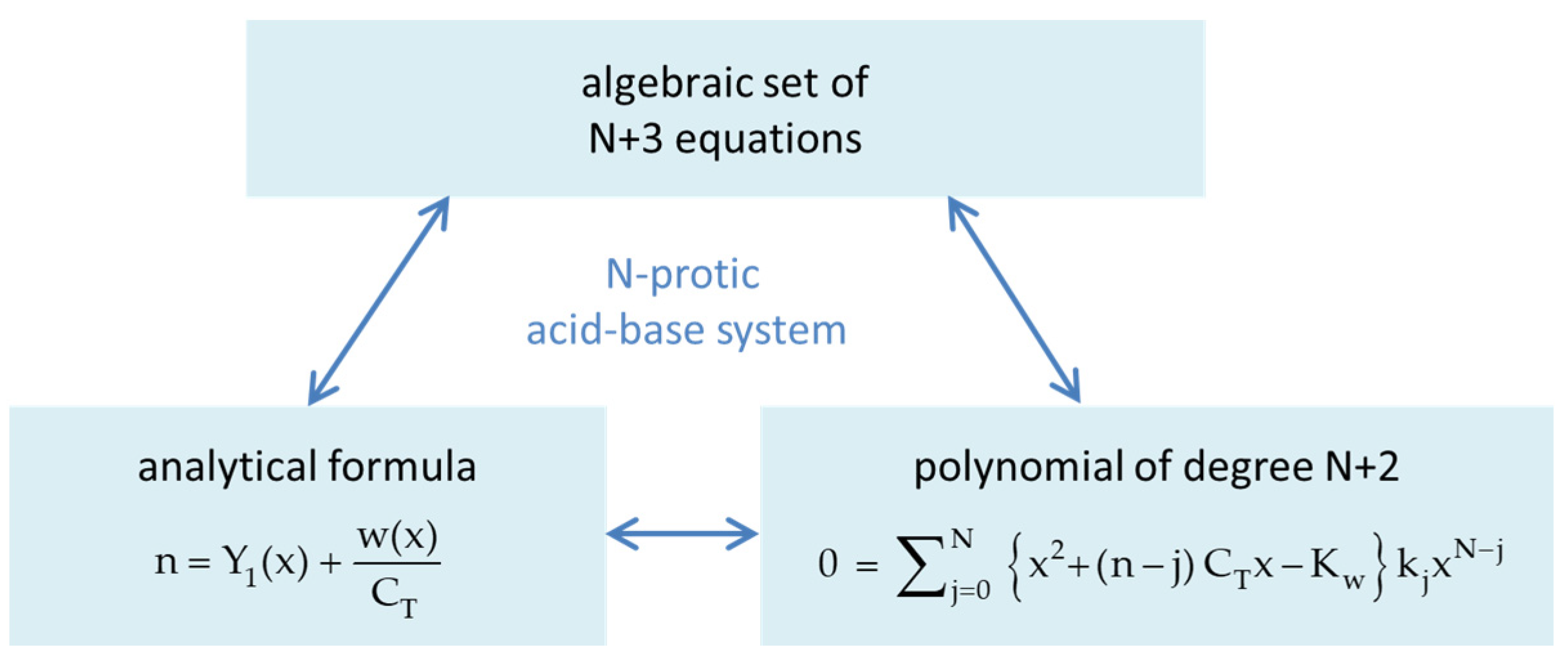
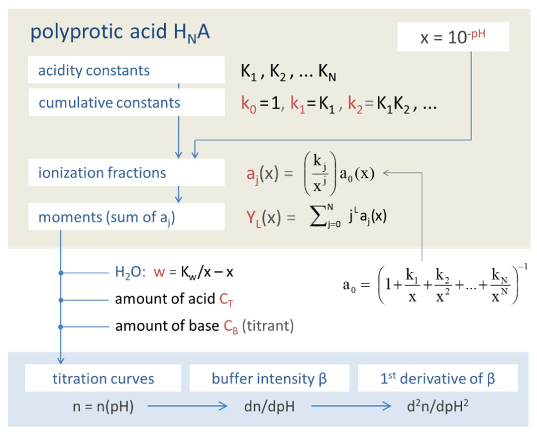
Table A1.
Special values of aj and YL at equivalence points.
| semi-EPn for Half-Integer n (j = n + ½) | EPn for Integer n (j = n) |
|---|---|
| pHn = pKj | pHn = pHj ≡ ½ (pKj + pKj+1) |
| aj = aj−1 ≈ ½ | aj = 1 − 2aj−1 (≈1) |
| YL = ½ {(j−1)L + jL} | YL ≈ jL |
| YL(pK1) = ½ | YL(pH1) = 1 |
| YL(pK2) = ½ (1 + 2L) | YL(pH2) = 2L |
| YL(pK3) = ½ (2L + 3L) | YL(pH3) = 3L |
| Y1(pKj) = j − ½ | Y1(pHj) = j |
| Y2(pKj) = j (j − 1) + ½ | Y2(pHj) = j2 |
Appendix C.2. pH Derivatives
The following list contains a set of important pH derivations:
References
- Stumm, W.; Morgan, J.J. Aquatic Chemistry, 3rd ed.; John Wiley & Sons: New York, NY, USA, 1996; ISBN 978-0-471-51185-4. [Google Scholar]
- Morel, F.M.M.; Hering, J.G. Principles and Applications of Aquatic Chemistry; Wiley: New York, NY, USA, 1993; ISBN 978-0-471-54896-6. [Google Scholar]
- Appelo, C.; Postma, D. Geochemistry, Groundwater and Pollution, 2nd ed.; Routledge: Boca Raton, FL, USA, 2010; ISBN 978-0-415-36428-7. [Google Scholar]
- Butler, J.N. Ionic Equilibrium: Solubility and pH Calculations, Rev; Wiley: New York, NY, USA, 1998; ISBN 0471585262. [Google Scholar]
- Harris, D.C. Quantitative Chemical Analysis, 8th ed.; Freeman Custom Publishing: New York, NY, USA, 2010; ISBN 1429264845. [Google Scholar]
- Hunter, K.A. Acid-Base Chemistry of Aquatic Systems: An Introduction to the Chemistry of Acid-Base Equilibria with Emphasis on the Carbon Dioxide System in Natural Waters; Department of Chemistry, University of Otago: Dunedin, New Zealand, 1998. [Google Scholar]
- Kahlert, H.; Scholz, F. Acid-Base Diagrams; Springer: Berlin/Heidelberg, Germany, 2013; ISBN 978-3-642-37901-7. [Google Scholar]
- Pardue, H.L.; Odeh, I.N.; Tesfai, T.M. Unified Approximations: A New Approach for Monoprotic Weak Acid-Base Equilibria. J. Chem. Educ. 2004, 81, 1367. [Google Scholar] [CrossRef]
- Casado-Riobó, A. A More Rational Treatment of the Acid-Base Equilibria Applying the Proton Condition in Equilibrium. How the Protons in Equilibria are Additive: Dissolutions of Acids. Crit. Rev. Anal. Chem. 2005, 35, 289–299. [Google Scholar] [CrossRef]
- Hofmann, A.F.; Soetaert, K.; Middelburg, J.J.; Meysman, F.J.R. AquaEnv: An Aquatic Acid–Base Modelling Environment in R. Aquat Geochem. 2010, 16, 507–546. [Google Scholar] [CrossRef] [Green Version]
- Parkhust, D.L.; Appelo, C. Description of Input and Examples for PHREEQC Version 3: A Computer Program for Speciation, Batch-Reaction, One-Dimensional Transport, and Inverse Geochemical Calculations; US Geological Survey: Denver, CO, USA, 2013.
- Kulik, D.A.; Wagner, T.; Dmytrieva, S.V.; Kosakowski, G.; Hingerl, F.F.; Chudnenko, K.V.; Berner, U.R. GEM-Selektor geochemical modeling package: Revised algorithm and GEMS3K numerical kernel for coupled simulation codes. Comput. Geosci. 2012. [Google Scholar] [CrossRef] [Green Version]
- Koukkari, P.; Pajarre, R. A Gibbs energy minimization method for constrained and partial equilibria. Pure Appl. Chem. 2011, 83, 1243–1254. [Google Scholar] [CrossRef]
- King, D.W.; Kester, D.R. A general approach for calculating polyprotic acid speciation and buffer capacity. J. Chem. Educ. 1990, 67, 932. [Google Scholar] [CrossRef]
- Weltin, E. Calculating Equilibrium Concentrations for Stepwise Binding of Ligands and Polyprotic Acid-Base Systems: A General Numerical Method to Solve Multistep Equilibrium Problems. J. Chem. Educ. 1993, 70, 568. [Google Scholar] [CrossRef]
- Rodriguez, J.L.; Loparo, K.A. Modeling and identification of pH processes. In Proceedings of the 2004 American Control Conference, Boston, MA, USA, 30 June–2 July 2004; IEEE: Piscataway, NJ, USA, 2004; Volume 6, pp. 5483–5488, ISBN 0-7803-8335-4. [Google Scholar]
- Hurek, J.; Nackiewicz, J. A Simple Method for the Consecutive Determination of Protonation Constants through Evaluation of Formation Curves. J. Chem. Educ. 2013, 90, 604–608. [Google Scholar] [CrossRef]
- Mioni, R.; Mioni, G. A Mathematical Model of pH, Based on the Total Stoichiometric Concentration of Acids, Bases and Ampholytes Dissolved in Water. Scand. J. Clin. Lab. Investig. 2015, 75, 452–469. [Google Scholar] [CrossRef]
- Gambi, A.; Toniolo, R. Acid-Base Logarithmic Diagrams with Computer Algebra Systems. ChemTexts 2016, 2, 9. [Google Scholar] [CrossRef] [Green Version]
- Simms, H.S. Dissociation of Polyvalent Substances II. Relation of Constants to Chemical Structure. J. Am. Chem. Soc. 1926, 48, 1251–1261. [Google Scholar] [CrossRef]
- Pehrsson, L. Acid-base titrations by stepwise addition of equal volumes of titrant with special reference to automatic titrations—II Theory of titration of mixtures of acids, polyprotic acids, acids in mixture with weak bases, and ampholytes. Talanta 1976, 23, 781–788. [Google Scholar] [CrossRef]
- de Levie, R. The Formalism of Titration Theory. Chem. Educator 2001, 6, 272–276. [Google Scholar] [CrossRef]
- Jano, I.; Hardcastle, J.; Jano, L.A.; Bates, K.R.; McCreary, H.E. General Equation for Determining the Dissociation Constants of Polyprotic Acids and Bases from Additive Properties: Part III. Calculation of Errors. Anal. Chim. Acta 2001, 428, 309–321. [Google Scholar] [CrossRef]
- Khan, A. A simple method for analysis of titration curves of polyprotic acids. Nucleus 2015, 51, 448–454. [Google Scholar]
- Asuero, A.G. Buffer Capacity of a Polyprotic Acid: First Derivative of the Buffer Capacity and pKa Values of Single and Overlapping Equilibria. Crit. Rev. Anal. Chem. 2007, 37, 269–301. [Google Scholar] [CrossRef]
- Asuero, A.G.; Michałowski, T. Comprehensive Formulation of Titration Curves for Complex Acid-Base Systems and Its Analytical Implications. Crit. Rev. Anal. Chem. 2011, 41, 151–187. [Google Scholar] [CrossRef]
- Michałowski, T.; Asuero, A.G. New Approaches in Modeling Carbonate Alkalinity and Total Alkalinity. Crit. Rev. Anal. Chem. 2012, 42, 220–244. [Google Scholar] [CrossRef]
- Michałowska-Kaczmarczyk, A.M.; Michałowski, T. Dynamic Buffer Capacity in Acid-Base Systems. J. Solut. Chem. 2015, 44, 1256–1266. [Google Scholar] [CrossRef] [PubMed] [Green Version]
- Kaczmarczyk, A.M.M.; Kucab, A.S.; Asuero, A.G.; Michalowski, T. The Simms Constants as Parameters in Hyperbolic Functions Related to Acid-Base Titration Curves. J. Chem. Appl. Chem. Eng. 2018, 2. [Google Scholar] [CrossRef]
- Michalowska-Kaczmarczyk, A.M.; Michalowski, T. Dynamic buffer capacity versus alkalinity. Formulation in terms of Simms constants idea. Biomed. Sci. Eng. 2020, 6, 1–9. [Google Scholar] [CrossRef]
- Schellman, J.A. Macromolecular binding. Biopolymers 1975, 14, 999–1018. [Google Scholar] [CrossRef]
- Wyman, J.; Gill, S.J. Binding and Linkage: Functionnal Chemistry of Biological Molecules; University Science Books: Mill Valley, CA, USA, 1990; ISBN 9780935702569. [Google Scholar]
- Onufriev, A.; Case, D.A.; Ullmann, G.M. A novel view of pH titration in biomolecules. Biochemistry 2001, 40, 3413–3419. [Google Scholar] [CrossRef] [PubMed]
- Ullmann, G.M. Relations between Protonation Constants and Titration Curves in Polyprotic Acids: A Critical View. J. Phys. Chem. B 2003, 107, 1263–1271. [Google Scholar] [CrossRef]
- Allison, J.D.; Brown, D.S.; Novo-Gradac, K.J. MINTEQA2/PRODEFA2, A Geochemical Assessment Model for Environmental Systems: User Manual Supplement for Version 4.0; EPA: Washington, DC, USA, 1998. [Google Scholar]
- Ball, J.W.; Nordstrom, D.K. WATEQ4F—User’s Manual with Revised Thermodynamic Data Base and Test Cases for Calculating Speciation of Major, Trace and Redox Elements in Natural Waters; US Geological Survey: Denver, CO, USA, 1991. [Google Scholar]
- Reif, F. Fundamentals of Statistical and Thermal Physics; McGraw-Hill: Boston, MA, USA, 1965; ISBN 978-0-07-051800-1. [Google Scholar]
- Kittel, C. Introduction to Solid State Physics, 4th ed.; John Wiley & Sons Ltd.: Hoboken, NJ, USA, 1971; ISBN 978-0-471-14286-7. [Google Scholar]
- Millero, F.J. Thermodynamics of the Carbon Dioxide System in the Oceans. Geochim. Cosmochim. Acta 1995, 59, 661–677. [Google Scholar] [CrossRef]
- RES³T- Rossendorf Expert System for Surface and Sorption Thermodynamics. Available online: https://www.hzdr.de/db/res3t.login (accessed on 15 August 2019).
Figure 1.
Equivalent fraction as the central quantity from which all other formulas follow.

Figure 2.
Relationships between 1-, 2-, and 3-component systems.

Figure 3.
pH dependence of ionization fractions for four acids (small circles mark equivalence points).
Figure 3.
pH dependence of ionization fractions for four acids (small circles mark equivalence points).

Figure 4.
Each ionization fraction aj has its own domain in the pH interval between two adjacent pKj values. (HA—acetic acid, H2A—carbonic acid, H3A—phosphoric acid).
Figure 4.
Each ionization fraction aj has its own domain in the pH interval between two adjacent pKj values. (HA—acetic acid, H2A—carbonic acid, H3A—phosphoric acid).

Figure 5.
Construction of Y1 (blue curve in bottom diagram) from summation over weighted ionization fraction aj. (Example: phosphoric acid as a triprotic acid).
Figure 5.
Construction of Y1 (blue curve in bottom diagram) from summation over weighted ionization fraction aj. (Example: phosphoric acid as a triprotic acid).

Figure 6.
pH dependence of the moments Y1 to Y4 for four acids. In the case of monoprotic acids (top-left diagram), all YL are equal, i.e., the four curves cover each other.
Figure 6.
pH dependence of the moments Y1 to Y4 for four acids. In the case of monoprotic acids (top-left diagram), all YL are equal, i.e., the four curves cover each other.

Figure 7.
Titration curve n = n(pH) of the “closed” carbonate system (100 mM H2CO3).

Figure 8.
Titration curves for 1, 10, and 100 mM H2CO3. (Left): n = n(pH); (right): pH = pH(n).

Figure 9.
Set of equations describing the 3-component acid–base system (H2O, HNA, strong base). The three components are coupled via the charge-balance equation.
Figure 9.
Set of equations describing the 3-component acid–base system (H2O, HNA, strong base). The three components are coupled via the charge-balance equation.

Figure 10.
Titration curves (i.e., buffer capacities) for four acids with different amounts of CT (including the high-CT limit n(pH) = Y1). Plots are based on Equation (41).
Figure 10.
Titration curves (i.e., buffer capacities) for four acids with different amounts of CT (including the high-CT limit n(pH) = Y1). Plots are based on Equation (41).

Figure 11.
Functional relationship between pH and CT for four acids (and n = 0). (Left): calculation based on Equation (43); (right): calculation based on the polynomial (44).
Figure 11.
Functional relationship between pH and CT for four acids (and n = 0). (Left): calculation based on Equation (43); (right): calculation based on the polynomial (44).

Figure 12.
Equivalence points of a triprotic acid—the common approach.

Figure 13.
Equivalence points of a triprotic acid H3A arranged on the pH scale.

Figure 14.
pH–CT diagrams for a diprotic and triprotic acid—the common approach.

Figure 15.
Relationship EPn ⇔ pHn. EPs and semi-EPs are located at integer and half-integer values of n on the titration curve. Calculation for 100 mM H2CO3.
Figure 15.
Relationship EPn ⇔ pHn. EPs and semi-EPs are located at integer and half-integer values of n on the titration curve. Calculation for 100 mM H2CO3.

Figure 16.
Two approaches to equivalence points.

Figure 17.
Normalized [ANC]n and [BNC]n for carbonic acid with CT = 10 mM.

Figure 18.
Optimal buffer range of the H2CO3 system with CT = 100 mM.

Figure 19.
Normalized buffer capacity (blue), buffer intensity (green), and dβ/dpH (red) for four acids and CT → ∞.
Figure 19.
Normalized buffer capacity (blue), buffer intensity (green), and dβ/dpH (red) for four acids and CT → ∞.

Figure 20.
Same as Figure 19, but for CT = 100 mM.
Figure 20.
Same as Figure 19, but for CT = 100 mM.

Figure 21.
Micro- and macrostates of a triprotic acid and the corresponding (cumulative) equilibrium constants.
Figure 21.
Micro- and macrostates of a triprotic acid and the corresponding (cumulative) equilibrium constants.

Figure 22.
Ionization fractions aj (dashed curves) and probability density functions f0 and fN.

Figure 23.
Interrelation between different types of equilibrium constants of a polyprotic acid HNA.

Figure 24.
Undissociated fraction a0 for strong and weak acids. Strong acids are completely dissociated in the pH range above pH ≈ 0.
Figure 24.
Undissociated fraction a0 for strong and weak acids. Strong acids are completely dissociated in the pH range above pH ≈ 0.

Figure 25.
Weak/strong vs. diluted/concentrated acids.

Figure 26.
Y1 and aj for a system composed of phosphoric and carbonic acid.

Figure 27.
pH–CT diagrams with trajectories of EPs and semi-EPs for four acids. Calculations are based on Equation (117).
Figure 27.
pH–CT diagrams with trajectories of EPs and semi-EPs for four acids. Calculations are based on Equation (117).

Figure 28.
Trajectories of EPs and semi-EPs for phosphoric acid (H3PO4) for the uncoupled (top) and coupled system (bottom).
Figure 28.
Trajectories of EPs and semi-EPs for phosphoric acid (H3PO4) for the uncoupled (top) and coupled system (bottom).

Figure 29.
Ionization fractions for phosphoric acid in two approximations (dashed lines) vs. exact description based on Equation (17).
Figure 29.
Ionization fractions for phosphoric acid in two approximations (dashed lines) vs. exact description based on Equation (17).

Figure 30.
Titration curve n = n(pH) for carbonic acid (CT = 10 mM) with equivalence points and the corresponding types of alkalinity and acidity.
Figure 30.
Titration curve n = n(pH) for carbonic acid (CT = 10 mM) with equivalence points and the corresponding types of alkalinity and acidity.

Figure 31.
Species distribution of H2CO3 as a function of pH for var A (left) and var B (right). Top diagrams: concentrations in linear scale; bottom diagrams: logarithmic scale.
Figure 31.
Species distribution of H2CO3 as a function of pH for var A (left) and var B (right). Top diagrams: concentrations in linear scale; bottom diagrams: logarithmic scale.

Figure 32.
Species distribution of H2CO3 as a function of pH for var A (left) and var C (right). Top diagrams: concentrations in linear scale; bottom diagrams: logarithmic scale.
Figure 32.
Species distribution of H2CO3 as a function of pH for var A (left) and var C (right). Top diagrams: concentrations in linear scale; bottom diagrams: logarithmic scale.

Figure 33.
pH–CT diagrams of the carbonic-acid system. (Left): H2CO3 in pure water (solid lines) vs. H2CO3 in seawater (dashed lines). (Right): closed-form expression (117) vs. numerical model (dots).
Figure 33.
pH–CT diagrams of the carbonic-acid system. (Left): H2CO3 in pure water (solid lines) vs. H2CO3 in seawater (dashed lines). (Right): closed-form expression (117) vs. numerical model (dots).

Figure 34.
Ionization fractions of two diprotic acids: glycine (left) vs. carbonic acid (right).

Figure 35.
Titration curves n = n(pH) for the amino acid glycine. (Left): calculations based on Equation (138) for four amounts of CT. (Right): comparison with numerical program PhreeqC (dots).
Figure 35.
Titration curves n = n(pH) for the amino acid glycine. (Left): calculations based on Equation (138) for four amounts of CT. (Right): comparison with numerical program PhreeqC (dots).

Figure 36.
Structural formula of four zwitterionic acids.

Figure 37.
Titration curves n(pH), buffer capacity β and its derivative dβ/dpH for four zwitterionic acids (from Table 12). Calculations for CT → ∞.
Figure 37.
Titration curves n(pH), buffer capacity β and its derivative dβ/dpH for four zwitterionic acids (from Table 12). Calculations for CT → ∞.

Figure 38.
Same as Figure 37, but for CT = 500 mM.
Figure 38.
Same as Figure 37, but for CT = 500 mM.

Figure 39.
(Left): Ionization fractions of EDTA in linear scale (top) and logarithmic scale (bottom). (Right): Titration curves of EDTA for three values of CT based on Equation (138). The red dots represent numerical calculations with PhreeqC. [Note: Complexation with Na is ignored.]
Figure 39.
(Left): Ionization fractions of EDTA in linear scale (top) and logarithmic scale (bottom). (Right): Titration curves of EDTA for three values of CT based on Equation (138). The red dots represent numerical calculations with PhreeqC. [Note: Complexation with Na is ignored.]

Figure 40.
Titration curve of glycine with EPs and semi-EPs located at integer and half-integer n.

Figure 41.
(Left) pH–CT diagrams for glycine. (Right): enlarged section around EP0 showing the isoelectric and isoionic points as a function of CT.
Figure 41.
(Left) pH–CT diagrams for glycine. (Right): enlarged section around EP0 showing the isoelectric and isoionic points as a function of CT.

Figure 42.
Ionization fractions representing the surface-species distribution on kaolinite (in the absence of Coulomb interactions).
Figure 42.
Ionization fractions representing the surface-species distribution on kaolinite (in the absence of Coulomb interactions).

Figure 43.
pH dependence of surface charge for four surfaces (in the absence of Coulomb interactions).
Figure 43.
pH dependence of surface charge for four surfaces (in the absence of Coulomb interactions).

Figure 44.
Three mathematically equivalent descriptions of the N-protic acid–base system. The algebraic set of N + 3 equations is defined in Equations (27)–(32).
Figure 44.
Three mathematically equivalent descriptions of the N-protic acid–base system. The algebraic set of N + 3 equations is defined in Equations (27)–(32).

Figure 45.
Building-block hierarchy of the acid–base model.

Table 1.
pK values for four N-protic acids at 25 °C. (The composite carbonic acid is the sum of the unionized species CO2(aq) and the pure acid: H2CO3* = CO2(aq) + H2CO3; to simplify the notation, we omit the asterisk (*) on H2CO3* throughout the paper).
Table 1.
pK values for four N-protic acids at 25 °C. (The composite carbonic acid is the sum of the unionized species CO2(aq) and the pure acid: H2CO3* = CO2(aq) + H2CO3; to simplify the notation, we omit the asterisk (*) on H2CO3* throughout the paper).
| N | Acid | Formula | Type | pK1 | pK2 | pK3 | Ref. |
|---|---|---|---|---|---|---|---|
| 1 | acetic acid | CH3COOH | HA | 4.76 | [35] | ||
| 2 | (composite) carbonic acid | H2CO3 | H2A | 6.35 | 10.33 | [36] | |
| 3 | phosphoric acid | H3PO4 | H3A | 2.15 | 7.12 | 12.35 | [35] |
| 3 | citric acid | C6H8O7 | H3A | 3.13 | 4.76 | 6.4 | [35] |
Table 2.
Two types of ionization fractions.
| Type 1 (S Shaped) | Type 2 (Bell Shaped) | |
|---|---|---|
| ionization fraction | a0 and aN | a1, a2, … aN−1 (does not exist for 1-protic acids) |
| domain (pH interval) | pH < pK1 (for a0) pH > pKN (for aN) | pKj < pH < pKj+1 |
| maximum at pH | −∞ (for a0) +∞ (for aN) | ½ (pKj + pKj+1) |
| strongly acidic (pH → 0) strongly alkaline (pH → 14) | a0 = 1, aN = 0 a0 = 0, aN = 1 | aj = 0 aj = 0 |
| integral (area below curve) | infinite | finite |
| statistical meaning (see Section 2.5.3) | cumulative distribution function | – |
| associated equivalence points | two external EPs: EP0 and EPN | N − 1 internal EPs: EP1, EP2, … EPN-1 |
Table 3.
Internal equivalence points (based on pK values in Table 1).
Table 3.
Internal equivalence points (based on pK values in Table 1).
| N | Acid | pH1/2 | pH1 | pH3/2 | pH2 | pH5/2 |
|---|---|---|---|---|---|---|
| 1 | acetic acid | 4.76 | ||||
| 2 | (composite) carbonic acid | 6.35 | 8.34 | 10.33 | ||
| 3 | phosphoric acid | 2.15 | 4.68 | 7.21 | 9.78 | 12.35 |
| 3 | citric acid | 3.13 | 3.94 | 4.76 | 5.58 | 6.4 |
Table 4.
Macroscopic and microscopic acidity constants.
| N Acidity Constants | N + 1 Cumulative Constants for | N Simms Constants | 2N − 1 Microscopic Constants | |
|---|---|---|---|---|
| Dissociation | Association | |||
| K1, K2, …, KN | k0 = 1 | β0 = 1 | g1, g2, …, gN | g1, g2, g3, … g1g2, g2g3, … g1g2g3, … g1g2⋯gN |
| (implicit functions of Equations (101) and (102)) | ||||
Table 5.
Strong vs. weak acids (greatly simplified).
| Strong Acid | Weak Acid | |
|---|---|---|
| acidity constant | Ka ≫ 1 | Ka ≤ 1 |
| pKa = −lg Ka | pKa < 0 | pKa > 0 |
| [H+] ≈ {H+} = 10−pH | [H+] ≈ CT | [H+] ≪ CT |
| undissociated acid | [HA] ≈ 0 or a0 ≈ 0 | [HA] ≈ CT or a0 ≈ 1 |
| dissociated acid | [A−] ≈ CT or a1 ≈ 1 | [A−] ≪ CT or a1 ≪ 1 |
Table 6.
Degree of strength vs. degree of dilution.
| Degree of Strength | Degree of Dilution | |||||
|---|---|---|---|---|---|---|
| determined by | acidity constant Ka | amount of acid CT | ||||
| relationships | weak acid small Ka (positive pKa | ↔ ↔ ↔ | strong acid large Ka negative pKa) | diluted acid small CT | ↔ ↔ | concentr. Acid large CT |
| compares | two different acids | dilution of the same acid | ||||
| describes | release of H+ | dilution of H+ | ||||
| type | fundamental property (cannot be changed) | control parameter (can be changed) | ||||
Table 7.
Equivalence points as local extrema and inflection points.
| Function/Curve | semi-EPn (half-integer n = j − ½) at pKj | EPn (integer n = j) at pHj |
|---|---|---|
| titration curve n = n(pH) (normalized buffer capacity) | inflection points | inflection points |
| buffer intensity β = dn/dpH | maxima | minima |
| dβ/dpH = d2n/dpH2 | zeros | zeros |
| ionization fraction aj | inflection point | maximum |
Table 8.
Thermodynamic and conditional equilibrium constants for H2CO3 in pure water and seawater (at 25 °C, 1 atm); cK values from [39].
Table 8.
Thermodynamic and conditional equilibrium constants for H2CO3 in pure water and seawater (at 25 °C, 1 atm); cK values from [39].
| Thermodynamic K (Pure Water, I = 0) | Conditional cK (Seawater, I = 0.7 M) | |
|---|---|---|
| pK1 | 5.18 | 6.0 |
| pK2 | 10.33 | 9.1 |
| pKw | 14.0 | 13.9 |
Table 9.
Diprotic acids (N = 2): ordinary acid vs. zwitterion (simplest amino acid).
| Diprotic Acid | Zwitterion (Simplest Amino Acid) | |||||
|---|---|---|---|---|---|---|
| 1st dissociation | H2A = H+ + HA− | K1 | H2A+ = H+ + HA | K1 | ||
| 2nd dissociation | HA− = H+ + A−2 | K2 | HA = H+ + A− | K2 | ||
| species | H2A | HA− | A−2 | H2A+ | HA | A− |
| abbreviation | [0] | [1] | [2] | [0] | [1] | [2] |
| ionic fraction aj | a0 | a1 | a2 | a0 | a1 | a2 |
| charge zj | 0 | −1 | -2 | 1 | 0 | −1 |
| average charge zav | (0·[H2A] − 1·[HA−] − 2·[A−2])/CT | (1·[H2A+] − 0·[HA] − 1·[A−])/CT | ||||
Table 10.
The three species of an ordinary diprotic acid vs. the simplest zwitterion.
| Diprotic Acid (Z = 0) | Zwitterion (Z = 1) | ||||
|---|---|---|---|---|---|
| [0]: | [H2A] | (neutral) | [H2A+] | (cation) | highest protonation |
| [1]: | [HA−] | (anion) | [HA] | (neutral) | |
| [2]: | [A−2] | (anion) | [A−] | (anion) | fully deprotonated |
Table 11.
Three exceptional cases out of N + 1 acid species.
| Ordinary Acid Z = 0 | Zwitterion 1 ≤ Z < N | |||
|---|---|---|---|---|
| j = 0 | [0] = [HNA+Z] | highest protonation | neutral | cation |
| j = Z | [Z] = [HN-ZA] | undissociated acid | neutral, [Z] = [0] | neutral |
| j = N | [N] = [A−(N−Z)] | fully deprotonated | anion | anion |
Table 12.
Acidity constants for carbonic acid and zwitterionic acids (the pK values for EDTA are taken from [5]; they differ slightly from those in [17]).
| Acid | N | Z | pK1 | pK2 | pK3 | pK4 | pK5 | pK6 | [j = 0] | [j = Z] | [j = N] |
|---|---|---|---|---|---|---|---|---|---|---|---|
| carbonic acid | 2 | 0 | 6.35 | 11.33 | H2A | H2A | A−2 | ||||
| glycine | 2 | 1 | 2.35 | 9.778 | H2A+ | HA | A−1 | ||||
| glutamic acid | 3 | 1 | 2.16 | 4.30 | 9.96 | H3A+ | H2A | A−2 | |||
| NTA | 4 | 1 | 1.0 | 2.0 | 2.942 | 10.28 | H4A+ | H3A | A−3 | ||
| EDTA | 6 | 2 | 0 | 1.5 | 2.16 | 3.119 | 6.281 | 10.94 | H6A+2 | H4A | A−4 |
Table 13.
Isoionic vs. isoelectric point.
| Isoionic Point | Isoelectric Point (pI) |
|---|---|
| pH of pure acid | pH at which the net charge of all acid species is zero |
| depends on CT (approaches pI-value for CT → ∞ and pH = 7 for CT → 0) | independent of CT |
| Z − Y1(pH) = w(pH)/CT | Z − Y1(pH) = 0 |
| exists for ordinary acids and zwitterions | exists only for zwitterions |
Table 14.
Intrinsic pK values and pHpzc for surface complexation on four (clay) minerals [40].
Table 14.
Intrinsic pK values and pHpzc for surface complexation on four (clay) minerals [40].
| Kaolinite | Mica | Goethite | Gibbsite | |
|---|---|---|---|---|
| pK1 | 2.52 | 6.01 | 7.13 | 7.53 |
| pK2 | 5.88 | 7.65 | 9.60 | 9.87 |
| pHpzc = ½ (pK1+pK2) | 4.20 | 6.83 | 8.37 | 8.70 |
Publisher’s Note: MDPI stays neutral with regard to jurisdictional claims in published maps and institutional affiliations. |
© 2021 by the author. Licensee MDPI, Basel, Switzerland. This article is an open access article distributed under the terms and conditions of the Creative Commons Attribution (CC BY) license (https://creativecommons.org/licenses/by/4.0/).
Share and Cite
MDPI and ACS Style
Kalka, H. Polyprotic Acids and Beyond—An Algebraic Approach. Chemistry 2021, 3, 454-508. https://doi.org/10.3390/chemistry3020034
AMA Style
Kalka H. Polyprotic Acids and Beyond—An Algebraic Approach. Chemistry. 2021; 3(2):454-508. https://doi.org/10.3390/chemistry3020034
Chicago/Turabian StyleKalka, Harald. 2021. "Polyprotic Acids and Beyond—An Algebraic Approach" Chemistry 3, no. 2: 454-508. https://doi.org/10.3390/chemistry3020034