Non-Parametric Retrieval of Aboveground Biomass in Siberian Boreal Forests with ALOS PALSAR Interferometric Coherence and Backscatter Intensity

Abstract

The main objective of this paper is to investigate the effectiveness of two recently popular non-parametric models for aboveground biomass (AGB) retrieval from Synthetic Aperture Radar (SAR) L-band backscatter intensity and coherence images. An area in Siberian boreal forests was selected for this study. The results demonstrated that relatively high estimation accuracy can be obtained at a spatial resolution of 50 m using the MaxEnt and the Random Forests machine learning algorithms. Overall, the AGB estimation errors were similar for both tested models (approximately 35 t∙ha⁻¹). The retrieval accuracy slightly increased, by approximately 1%, when the filtered backscatter intensity was used. Random Forests underestimated the AGB values, whereas MaxEnt overestimated the AGB values.

1. Introduction

Aboveground biomass (AGB) is an important variable in carbon accounting and climate science. In particular, forest AGB is relevant because forests constitute approximately 70%–90% of the Earth’s aboveground biomass [1].

The AGB is defined as the mass of living organic matter growing above ground level per unit area at a particular time. The difference in AGB over time allows for measurement of carbon sequestration (excluding root growth) and carbon emission from deforestation, forest degradation, and forest fires. The estimation of AGB in the boreal forest is of special concern as it constitutes the largest biome in the world and has substantial carbon accumulation capability. Russia, as the country with the largest forested area in the world (809 million ha [2]), provided more than 90% of the carbon sink of the world’s boreal forests between the years 2000 and 2007 [3]. Despite this importance, Russia’s boreal forest has the highest uncertainty in carbon stock calculations [4,5]. This is mostly due to poor measurements of biomass stocks, forest degradation, deforestation, and forest growth. Additionally, due to the lack of financial support, some forested regions in Siberia have not been inventoried for more than 20 years [6]. Therefore, there is a strong need for earth observation-based methods to reduce costs and improve biomass estimations.

The most common method of measuring AGB is estimation from field measurements, such as stem diameter and tree height, using allometric models. However, due to the sampling nature of the field measurements and their high acquisition costs, they can only be collected over small areas. Satellite technology together with reliable in situ measurements allows for accurate and relatively cost-efficient wall-to-wall AGB estimates.

There are different remote sensing techniques for AGB retrieval. Several publications provide a comprehensive review of use of remote sensing techniques for biomass estimation including sourcebooks of recommended methods and data sources [7,8,9,10,11,12,13,14,15,16]. The estimates using optical sensors are feasible at low biomass levels using vegetation indices, bidirectional reflectance distribution function (BRDF), and texture [17,18,19,20,21,22]. The latest results of biomass estimation using Landsat data showed that an accuracy of ±36% can be measured in the boreal zones [23]. The most accurate estimates are gathered from airborne light detection and ranging (LiDAR) systems. The only archive data from the satellite profiling LiDAR for measuring and monitoring vegetation are from the Ice, Cloud, and land Elevation (ICESat) Geoscience Laser Altimeter System (GLAS). However, the data have some limitations related to the large footprint, sparse coverage, and sensitivity to terrain variability [24,25,26,27,28]. Another technique that has a potential for forest AGB estimation is synthetic aperture radar (SAR). Similar to LiDAR sensors, radar systems are sensitive to the geometrical properties of observed objects; on the contrary, SAR platforms are imaging sensors. SAR is an active system that transmits microwave energy at wavelengths ranging from 3.1 cm (the X band) to 23.6 cm (the L band). Longer wavelengths, i.e., L-band, are preferable due to its deeper penetration into the forest canopy and due to saturation of radar signal at higher biomass levels [29,30,31]. Especially, SAR data with long wavelength, horizontal and vertical polarizations, interferometric capabilities, and global acquisition strategy are of great value for biomass retrieval. Data from those sensors are already available as archive data from L-band Japanese Earth Resources Satellite 1 (JERS-1) and Advanced Land Observing Satellite (ALOS) Phased Array L-band Synthetic Aperture Radar (PALSAR), or as new acquisitions from ALOS-2 PALSAR-2. Moreover, new SAR missions are planned that will ensure data continuity, e.g., the European Space Agency’s P-band (68.9 cm) BIOMASS mission [32] and the UK NovaSAR S-band mission [33].

SAR data have been investigated for more than 30 years and were proved to be physically related to forest parameters until the saturation point showing correlation coefficients of up to approximately 0.9 [29,34,35,36]. Many SAR properties have been successfully exploited to quantify biomass: backscattering intensity [37,38], interferometric phase [39,40], interferometric correlation [41,42,43], polarimetric signature [44,45], SAR tomography, and radargrammetry [46,47,48]. In particular, satellite SAR data at the L-band have provided low AGB or growing stock volume (GSV) estimation error down to approximately 20% when forest stands greater than 10 ha were used and/or a multi-temporal approach was implemented [31,49,50,51,52]. Until now, only few retrieval results using interferometric coherence synergistically with backscatter over Russian boreal forests have been published [50,53,54].

Table 1 [50,51,52,55,56,57,58,59,60] presents a summary of the SAR retrieval statistics reported in the literature over Russian boreal forests, the same type of forest that was used in this study. The estimation error is represented as the root mean square error (RMSE) and the relative RMSE, i.e., the RMSE divided by the mean GSV or AGB.

Table 1. Summary of previous studies of growing stock volume (GSV) or aboveground biomass (AGB) estimation over Siberian boreal forests using SAR data. The estimation error is given as the root mean square error (RMSE) and the relative RMSE, i.e., the RMSE divided by the mean GSV or AGB.

Reference	SAR Sensor Wavelength	Estimated Variable	Model	Predictors	Spatial Resolution	Estimation Error RMSE (Units As Estimated Variable)/Relative RMSE (%)
[55]	JERS-1 L-band	GSV (m3∙ha−1)	Semi-empirical Water-Cloud type model	Backscatter in σ°HH, 9 images	Stand-wise > 8 ha	57–87/33–51
[50]	ERS-1/2 C-band	GSV (m3·ha−1)	Semi-empirical model Interforemetric Water Cloud Model	Interferometric coherence adjusted by environmental conditions (relative stocking, stand size, topography)	Stand-wise > 3 ha	45–75/25–41
[56]	Envisat ASAR C-band	GSV (m3·ha−1)	BIOMASAR—semi-empirical Water-Cloud type model	Backscatter in γ°HH and γ°VV polarization, tens of images	1 km	-/34.2
[57]	Envisat ASAR C-band	GSV (m3·ha−1)	BIOMASAR—semi-empirical Water-Cloud type model	Backscatter in γ°HH and γ°VV, mean 93 observations	0.5°	-/15
[51]	ALOS PALSAR L-band	AGB (t·ha−1)	Single and multivariate regression, semi-empirical Water-Cloud type model	Backscatter in σ°HH and σ°VV, 1-5 images	Stand-wise > 10 ha	46–55/25–32
[58,59]	ALOS PALSAR L-band	GSV (m3·ha−1)	Machine learning approach—Random Forest	4 ALOS PALSAR mosaics, backscatter in γ°HH and γ°HV	25 m	54.4/39.4
[52]	ALOS PALSAR L-band	GSV (m3·ha−1)	Empirical exponential model	Polarimetric coherence, HHVV-coherence	Stand-wise > 2 ha	33–51/-
[60]	ALOS PALSAR L-band	AGB (t·ha−1)	Machine learning approach—MaxEnt	ALOS PALSAR mosaic, backscatter in γ°HH and γ°HV, Landsat bands, and categorical data	50 m	36.4/-

Table 1. Summary of previous studies of growing stock volume (GSV) or aboveground biomass (AGB) estimation over Siberian boreal forests using SAR data. The estimation error is given as the root mean square error (RMSE) and the relative RMSE, i.e., the RMSE divided by the mean GSV or AGB.

Reference	SAR Sensor Wavelength	Estimated Variable	Model	Predictors	Spatial Resolution	Estimation Error RMSE (Units As Estimated Variable)/Relative RMSE (%)
[55]	JERS-1 L-band	GSV (m3∙ha−1)	Semi-empirical Water-Cloud type model	Backscatter in σ°HH, 9 images	Stand-wise > 8 ha	57–87/33–51
[50]	ERS-1/2 C-band	GSV (m3·ha−1)	Semi-empirical model Interforemetric Water Cloud Model	Interferometric coherence adjusted by environmental conditions (relative stocking, stand size, topography)	Stand-wise > 3 ha	45–75/25–41
[56]	Envisat ASAR C-band	GSV (m3·ha−1)	BIOMASAR—semi-empirical Water-Cloud type model	Backscatter in γ°HH and γ°VV polarization, tens of images	1 km	-/34.2
[57]	Envisat ASAR C-band	GSV (m3·ha−1)	BIOMASAR—semi-empirical Water-Cloud type model	Backscatter in γ°HH and γ°VV, mean 93 observations	0.5°	-/15
[51]	ALOS PALSAR L-band	AGB (t·ha−1)	Single and multivariate regression, semi-empirical Water-Cloud type model	Backscatter in σ°HH and σ°VV, 1-5 images	Stand-wise > 10 ha	46–55/25–32
[58,59]	ALOS PALSAR L-band	GSV (m3·ha−1)	Machine learning approach—Random Forest	4 ALOS PALSAR mosaics, backscatter in γ°HH and γ°HV	25 m	54.4/39.4
[52]	ALOS PALSAR L-band	GSV (m3·ha−1)	Empirical exponential model	Polarimetric coherence, HHVV-coherence	Stand-wise > 2 ha	33–51/-
[60]	ALOS PALSAR L-band	AGB (t·ha−1)	Machine learning approach—MaxEnt	ALOS PALSAR mosaic, backscatter in γ°HH and γ°HV, Landsat bands, and categorical data	50 m	36.4/-

The study presented in this paper is based on multi-temporal ALOS PALSAR L-band backscatter intensity and coherence data. Both types of data were used as explanatory variables for AGB retrieval at a local scale of 0.25 ha. The AGB was estimated using two non-parametric machine learning algorithms: maximum entropy (MaxEnt) and Random Forests. Both models are popular in applied research. The MaxEnt approach [61] is particularly popular in species distribution modeling [62,63]. However, the method was also successfully implemented for AGB estimation at regional and global scale [60,64]. The Random Forests [65] are widely used for classification in ecology [66,67,68] as well as for AGB estimation [27,58,69,70,71,72,73,74]. The Random Forests were found to be superior to other methods such as support vector machine (SVM), k-nearest neighbour (KNN), Gaussian processes (GP), and stepwise linear models [75]. So far Random Forests have not been compared with the MaxEnt approach.

In summary, the aim of this paper is to:

• use SAR L-band backscatter and coherence data synergistically to improve AGB estimation at a local scale;
• compare AGB retrieval results using two recently popular machine learning algorithms.

2. Test Site and Available Data

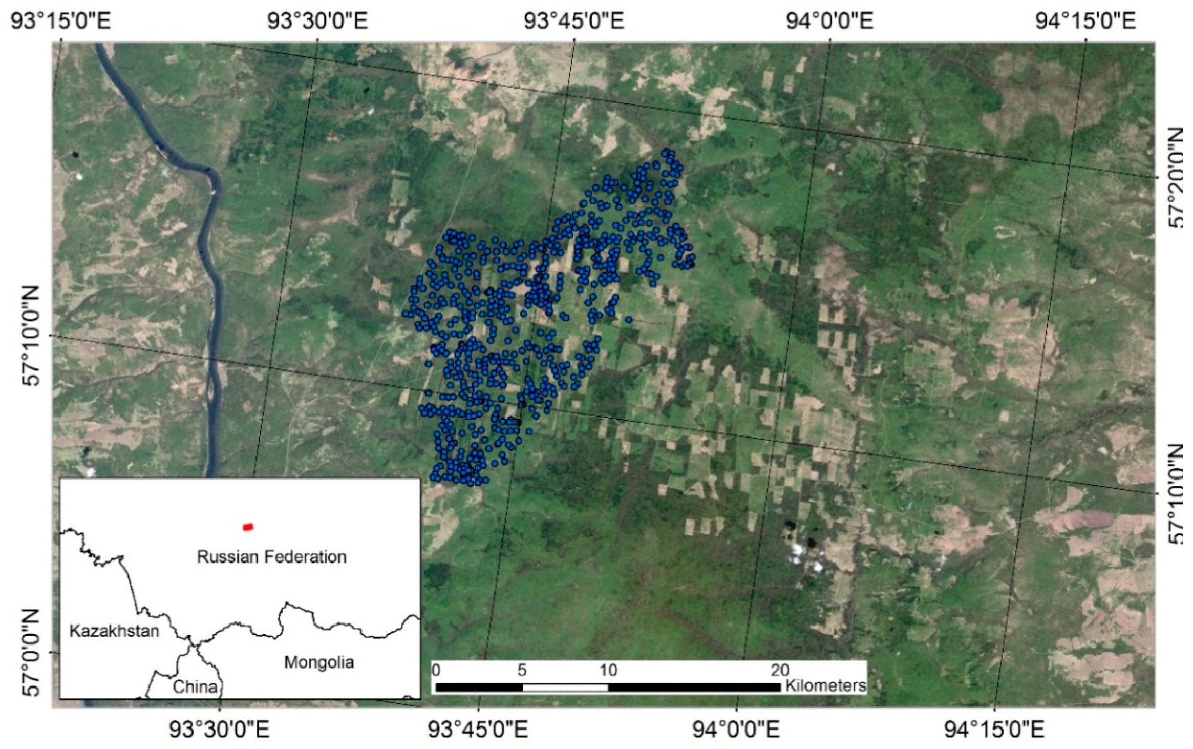
2.1. Study Site

The study site is located in Krasnoyarskiy Kray in the Southern part of Central Siberia, Russia, approximately 120 km northeast of the city Krasnoyarsk—part of the Bolshe Murtinsky forest enterprise (center coordinates: 57°12′N and 93°49′E, Figure 1). The area is characterized by a continental climate with long, severe winters and short, warm, and wet summers. From mid-October until the beginning of April, the mean temperature is approximately −15 °C; in summer the mean temperature is approximately +15 °C. The annual precipitation is below 450 millimeters.

Figure 1. Extent of the study area and the spatial distribution of the reference points. Background image acquired by the Landsat 5 TM satellite (data available from the U.S. Geological Survey Earth Explorer).

Figure 1. Extent of the study area and the spatial distribution of the reference points. Background image acquired by the Landsat 5 TM satellite (data available from the U.S. Geological Survey Earth Explorer).

The research area covers almost 2000 km². The area is mainly characterized by needleleaf, coniferous forests. The dominant trees are pine, spruce, fir, and larch. The main disturbances are logging activities and fire events. The study site is characterized by gentle topography with heights from 90 m to 572 m above sea level (a.s.l.) with an average height of 243 m a.s.l. The slopes range from 0° to 54° (riverside), with a mean value of 6°.

2.2. Available Data

The ALOS PALSAR L-band data were used for the explanatory variables. The data were delivered in Single Look Complex (SLC) Level 1.1 format. The data were provided by the Japan Aerospace Exploration Agency (JAXA) within the third phase of the Kyoto and Carbon Initiative [76,77]. In total, 19 scenes were available for this study area (Table 2). The weather data were downloaded from http://www.sibessc.uni-jena.de/ [78].

Ten scenes were acquired between 2006 and 2011 in fine beam single (FBS) mode and nine scenes were obtained in fine beam dual (FBD) mode. In the case of the FBS mode, the data were collected in horizontally transmitted and horizontally received polarization (HH), and in the case of the FBD mode, the data were given in HH and horizontally transmitted and vertically received (HV) polarizations.

The spatial resolution of the single-look image is 9.37 m in range and 3.14 m in azimuth for data acquired in the FBD mode and 4.68 m in range and 3.14 m in azimuth for data acquired in the FBS mode. The acquisition angle is 34.3°.

The forest inventory data were used as the dependent variable. The field data were provided by the Russian State Forest Inventory within the SIBERIA project [79]. The inventory dates back to 1998. Because of the time difference between inventory data and the SAR data acquisitions (>10 years) the field data were updated using semi-empirical phytomass models [80] and growth (yield) tables [81]. The latter were developed by the International Institute for Applied Systems Analyses (IIASA) in collaboration with the V.N. Sukachev Institute of Forest, Siberian Branch, Russian Academy of Sciences, and Moscow State Forest University. Those models and tables are recommended for use in forestry and forest management in Russia (Protocol of the Council of Federal Agency of Forest Management No. 2, dated 8 June 2006) [81].

The original data were gathered in the framework of the Russian forest inventory and planning (FIP) and are available in GIS vector format. Attributes such as GSV, age, tree height, diameter at breast height, and species composition were provided. All information is given for a forest stand, i.e. a group of trees occupying a specific area uniform in species composition, size, age, and management strategy. In total, information about 1604 stands was available.

Table 2. Summary of SAR data available for the test site. The data acquisition time was approximately 16 GMT—10 PM local time in summer or 11 PM local time in winter. The weather parameters are given as a mean from eight daily measurements [78]. The weather station is located approximately 50 km southwest from the center of the test site.

Image Name	Acquisition Date	Acquisition Mode	Weather Conditions: Mean Temperature (°C)/Wind Speed (m/s)/Precipitation (mm)/Snow Depth (mm)
ALPSRP049391140	28 December 2006	FBS	dry frozen conditions, −17.8/0.5/0/238.8
ALPSRP056101140	12 February 2007	FBS	dry frozen conditions, −18.9/1.7/0/340.4
ALPSRP082941140	15 August 2007	FBD	wet unfrozen conditions, 13.6/1.2/0/0 (2 days before heavy rain)
ALPSRP089651140	30 September 2007	FBD	wet unfrozen conditions, 13.1/3.9/-/0 (3 days before heavy rain)
ALPSRP103071140	31 December 2007	FBS	dry frozen conditions, −5.9/4.4/0/279.4
ALPSRP109781140	15 February 2008	FBD	dry frozen conditions, −17.2/0.4/0/381
ALPSRP129911140	2 July 2008	FBD	wet unfrozen conditions, 19.7/1.7/0.3/0
ALPSRP136621140	17 August 2008	FBD	wet unfrozen conditions, 16.8/1.6/0.8/0
ALPSRP156751140	2 January 2009	FBS	dry frozen conditions, −12.7/1.1/0/299.7
ALPSRP163461140	17 February 2009	FBS	dry frozen conditions, -31.3/0.6/0/459.7
ALPSRP190301140	20 August 2009	FBD	wet unfrozen conditions,14.7/0.8/1/0 (6 days before heavy rain)
ALPSRP197011140	5 October 2009	FBD	dry unfrozen conditions,11.5/1.6/0/0
ALPSRP210431140	5 January 2010	FBS	dry frozen conditions, −33.7/1.5/0/589.3
ALPSRP217141140	20 February 2010	FBS	dry frozen conditions, −22.9/1.2/0/599.4
ALPSRP243981140	23 August 2010	FBD	dry unfrozen conditions, 22.6/2.3/0/0
ALPSRP250691140	8 October 2010	FBD	wet unfrozen conditions, 1.4/1.7/0.5/10.2
ALPSRP257401140	23 November 2010	FBD	dry frozen conditions, −12.9/1.7/0/119.4
ALPSRP264111140	8 January 2011	FBS	dry frozen conditions, −23.3/1.5/0/360.7
ALPSRP270821140	23 February 2011	FBS	dry frozen conditions, −27.6/0.5/0/429.3

Table 2. Summary of SAR data available for the test site. The data acquisition time was approximately 16 GMT—10 PM local time in summer or 11 PM local time in winter. The weather parameters are given as a mean from eight daily measurements [78]. The weather station is located approximately 50 km southwest from the center of the test site.

Image Name	Acquisition Date	Acquisition Mode	Weather Conditions: Mean Temperature (°C)/Wind Speed (m/s)/Precipitation (mm)/Snow Depth (mm)
ALPSRP049391140	28 December 2006	FBS	dry frozen conditions, −17.8/0.5/0/238.8
ALPSRP056101140	12 February 2007	FBS	dry frozen conditions, −18.9/1.7/0/340.4
ALPSRP082941140	15 August 2007	FBD	wet unfrozen conditions, 13.6/1.2/0/0 (2 days before heavy rain)
ALPSRP089651140	30 September 2007	FBD	wet unfrozen conditions, 13.1/3.9/-/0 (3 days before heavy rain)
ALPSRP103071140	31 December 2007	FBS	dry frozen conditions, −5.9/4.4/0/279.4
ALPSRP109781140	15 February 2008	FBD	dry frozen conditions, −17.2/0.4/0/381
ALPSRP129911140	2 July 2008	FBD	wet unfrozen conditions, 19.7/1.7/0.3/0
ALPSRP136621140	17 August 2008	FBD	wet unfrozen conditions, 16.8/1.6/0.8/0
ALPSRP156751140	2 January 2009	FBS	dry frozen conditions, −12.7/1.1/0/299.7
ALPSRP163461140	17 February 2009	FBS	dry frozen conditions, -31.3/0.6/0/459.7
ALPSRP190301140	20 August 2009	FBD	wet unfrozen conditions,14.7/0.8/1/0 (6 days before heavy rain)
ALPSRP197011140	5 October 2009	FBD	dry unfrozen conditions,11.5/1.6/0/0
ALPSRP210431140	5 January 2010	FBS	dry frozen conditions, −33.7/1.5/0/589.3
ALPSRP217141140	20 February 2010	FBS	dry frozen conditions, −22.9/1.2/0/599.4
ALPSRP243981140	23 August 2010	FBD	dry unfrozen conditions, 22.6/2.3/0/0
ALPSRP250691140	8 October 2010	FBD	wet unfrozen conditions, 1.4/1.7/0.5/10.2
ALPSRP257401140	23 November 2010	FBD	dry frozen conditions, −12.9/1.7/0/119.4
ALPSRP264111140	8 January 2011	FBS	dry frozen conditions, −23.3/1.5/0/360.7
ALPSRP270821140	23 February 2011	FBS	dry frozen conditions, −27.6/0.5/0/429.3

3. Processing Methods

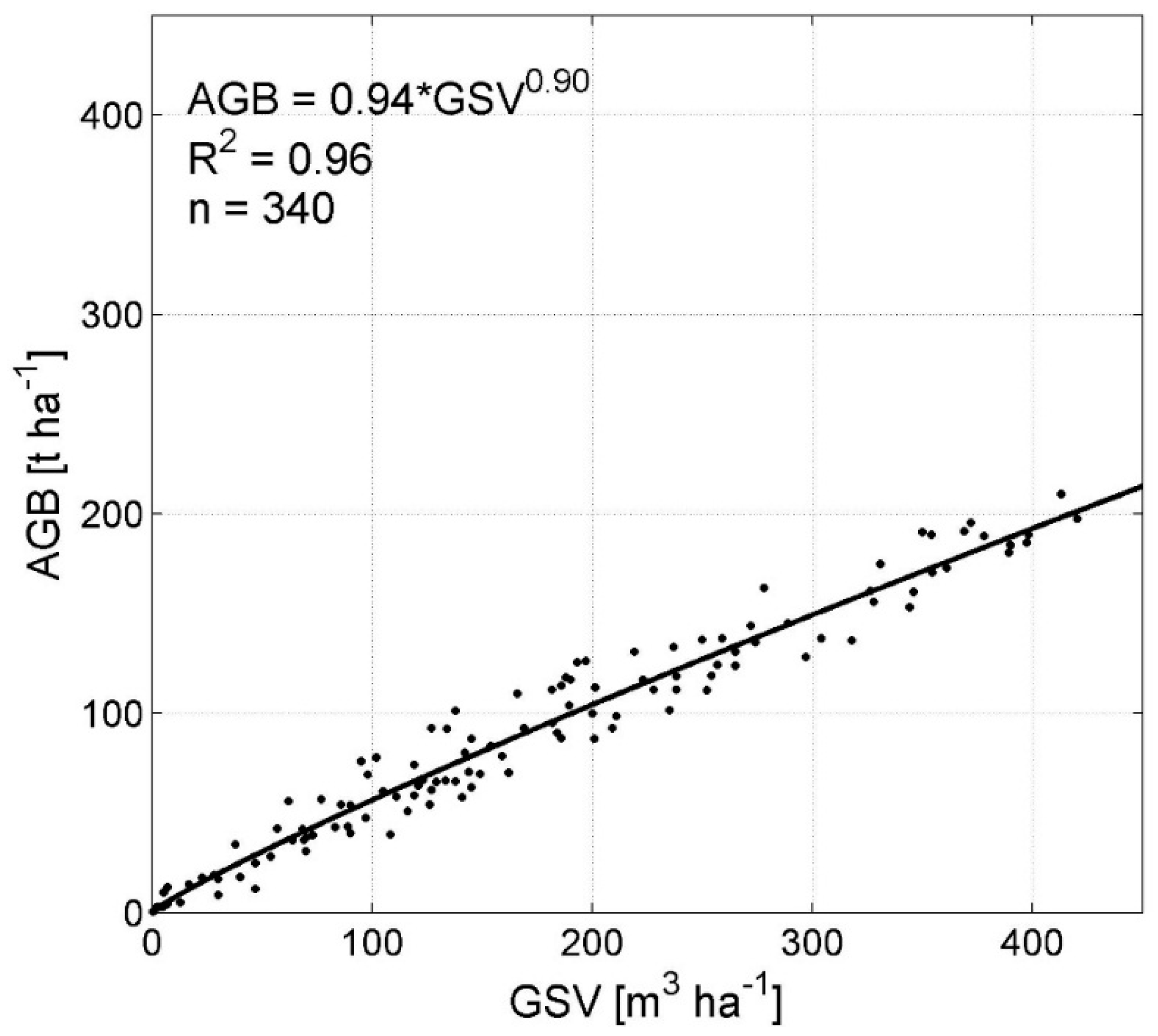
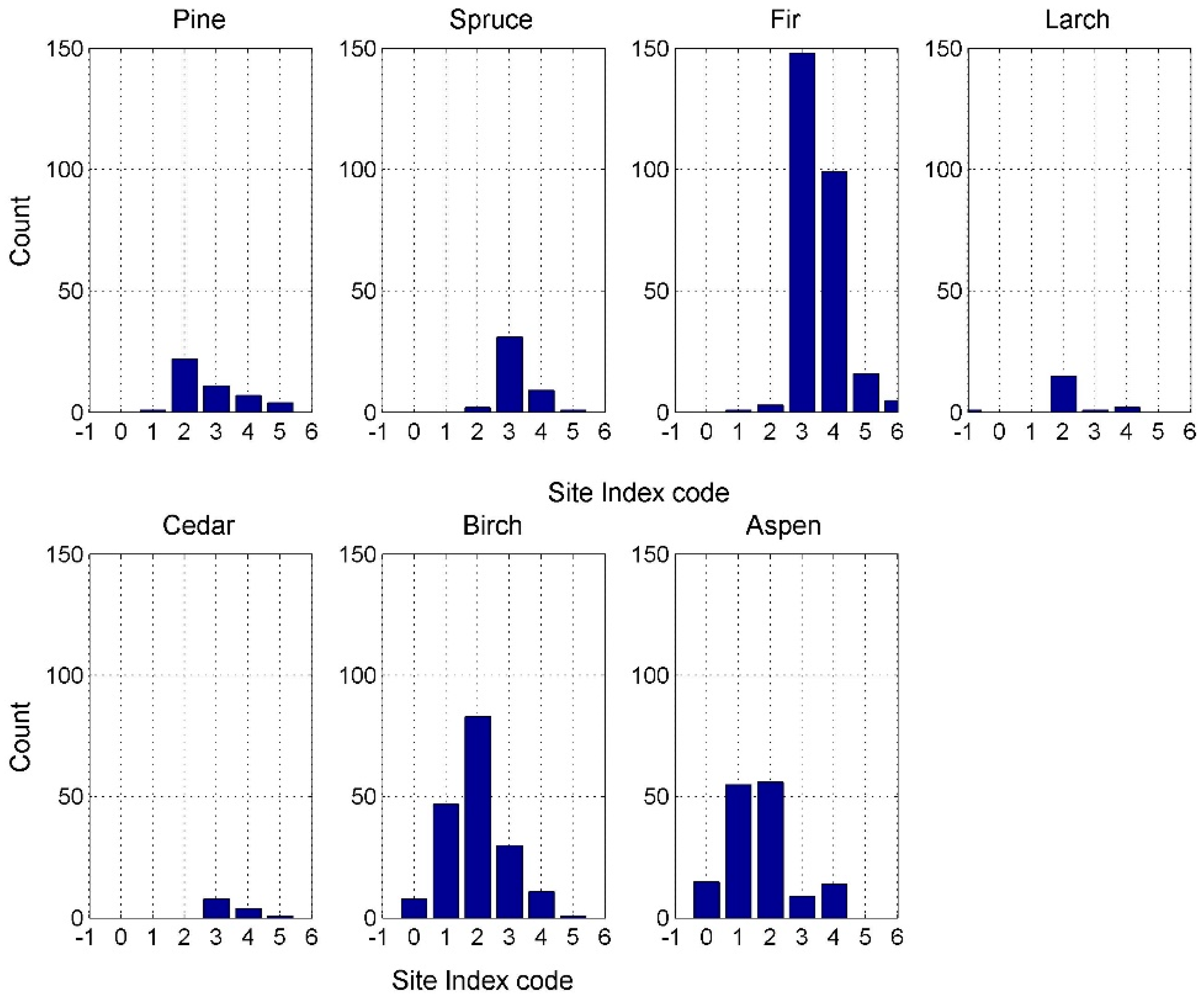
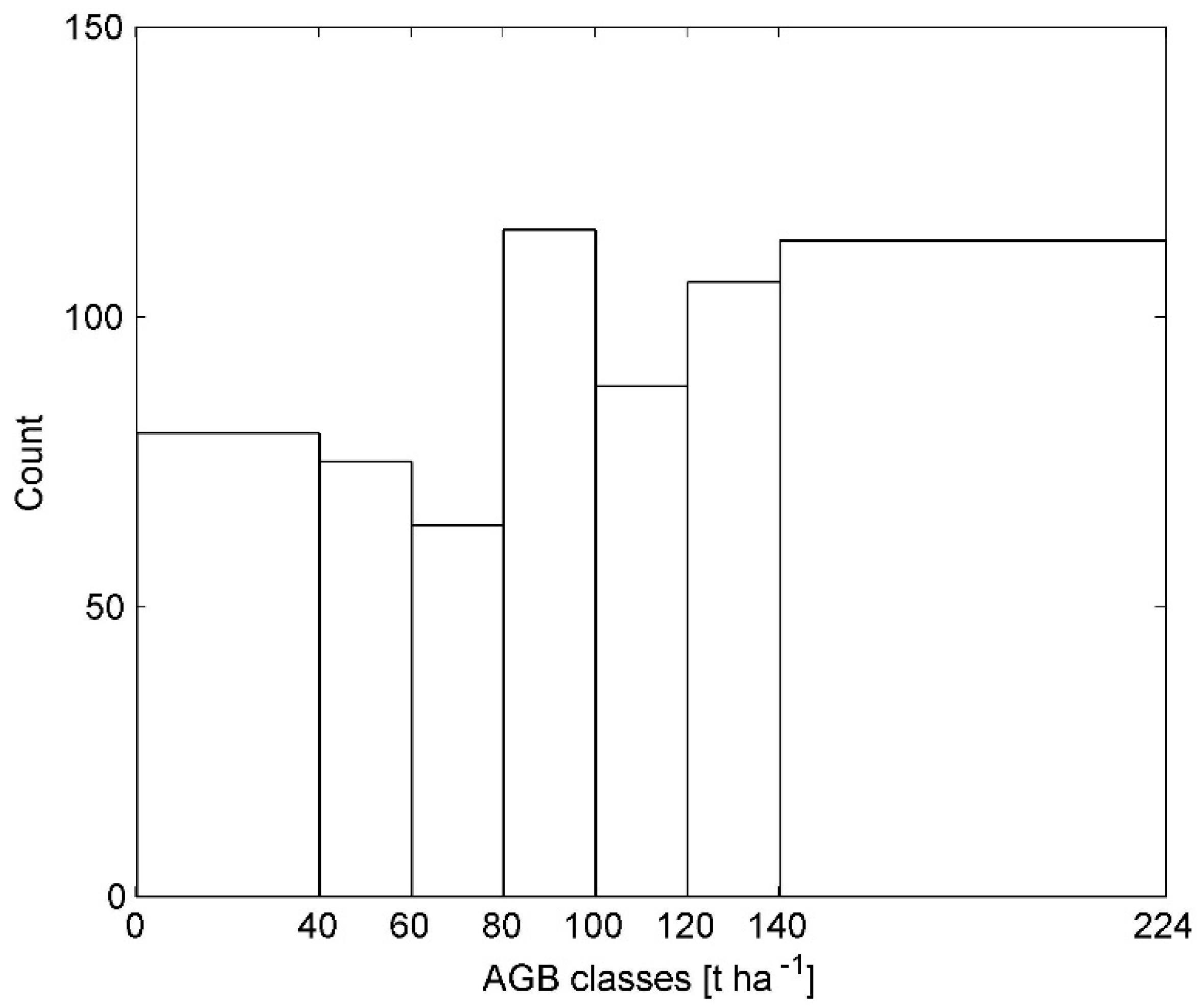
3.1. Forest Inventory Data

The available forest inventory data are for 1998. Therefore, the first step of AGB retrieval was an update of the reference data. The data were improved to the year 2010. The data update consisted of four stages. First, the forest stands that changed from forest to non-forest were excluded by visual interpretation using very high and high resolution optical data. Cloud-free images were selected from KOMPSAT-2 and RapidEye. The data were acquired from spring to autumn in 2010, 2011, and 2012. Then, from the resulting stands only those were selected in which at least 60% of the trees belong to a single species. The reason for the selection is that the growth (yield) tables were done for dominant tree species. In the second step, the stands were used in the semi-empirical phytomass models. The basis for the improvement of the old inventory data is a site index (SI). SI is defined as the edaphic and climatic characteristics of a site that have an impact on the growth and yield of a given tree species [82]. Usually SI classes are determined by the relationship between the mean tree height and the mean age of a stand. As the SI was not available in the original forest inventory data it was calculated from the following equation [83]:

$$H_t=22.47{\left(1-e^{-0.0234\mathrm{A}\left(1-e^{-0.0057A}\right)}\right)}^{0.548}+\left(3-SI\right)\mathsf{\Delta }$$

(1)

$$\mathsf{\Delta }=4.35{\left(1-e^{-0.0205\mathrm{A}}\right)}^{0.957}$$

(2)

where $H_t$represents tree height, $\mathrm{A}$ denotes forest stand age, and $\mathsf{\Delta }$ is the interval between site indexes.

In the case of Russian forests, the SI from Ib, Ia, I–V, Va, and Vb are denoted as where the class with the lowest SI indicates the best site conditions for forest trees to grow. The site indexes II and III are dominant in the study area with fir, birch, and aspen as the dominant species (Figure 2).

Figure 2. The number of stands with more than 60% of tree species per site index; site index code: −1-Ib, 0–Ia, 1–I, 2-II, 3-III, 4-IV, 5-V, 6-Va.

Figure 2. The number of stands with more than 60% of tree species per site index; site index code: −1-Ib, 0–Ia, 1–I, 2-II, 3-III, 4-IV, 5-V, 6-Va.

After calculating the SI, the growth rate was derived by implementing the Richards–Chapman growth function in polynomial quadratic form [81]:

$$GS{V}_{growthrate}=c_1{c}_2{c}_3{\left(1-e^{-c_{2}A}\right)}^{c_3-1}{e}^{-c_{2}A},$$

(3)

where $A$ denotes age and $c_i$are the parameters that have an ecological interpretation and depend on site index ($SI$) [81]:

$$c_i=c_{i3}S{I}^2+c_{i2}SI+c_{i1}.$$

(4)

After obtaining the GSV growth rate, the correction coefficient $GS{V}_{cc}$ was calculated:

$$GS{V}_{cc}=\frac{GS{V}_{in-situ}}{GS{V}_{model}}$$

(5)

where $GS{V}_{in-situ}$ represents the GSV measured in the field, whereas $GS{V}_{model}$ is the GSV calculated according to the models [81] for a particular site index and forest stand age. A new GSV was then derived:

$$GS{V}_{new}=GS{V}_{in-situ}+A_{diff}GS{V}_{growthrate}GS{V}_{cc}$$

(6)

where $A_{diff}$is the age difference between the old inventory and reference year 2010 and equals 12.

Thirdly, GSV were converted to AGB. Based on freely available in situ measurements of forest live biomass (phytomass) [83], a regional allometric model relating GSV to AGB was developed (Figure 3).

The final step of the reference data processing was to rasterize the inventory data to 50 m spatial resolution, and then to erode the stands. An erosion of two pixels was used (100 m) to avoid border effects in the SAR products. Then, the stands were converted into points using the center of gravity (centroid) of the stand. The final updated AGB values ranged from 0 to 224 t·ha⁻¹, with a mean value of 98 t·ha⁻¹. The stand size with erosion varied from 0.5 to 130 ha, with a mean value of 16 ha that corresponds to 64 pixels. The stand age varied from 20 to 290 years. Six hundred forty-one stands remained for the investigations.

Figure 3. Allometric model relating AGB to GSV using in situ measurements of forest phytomass.

Figure 3. Allometric model relating AGB to GSV using in situ measurements of forest phytomass.

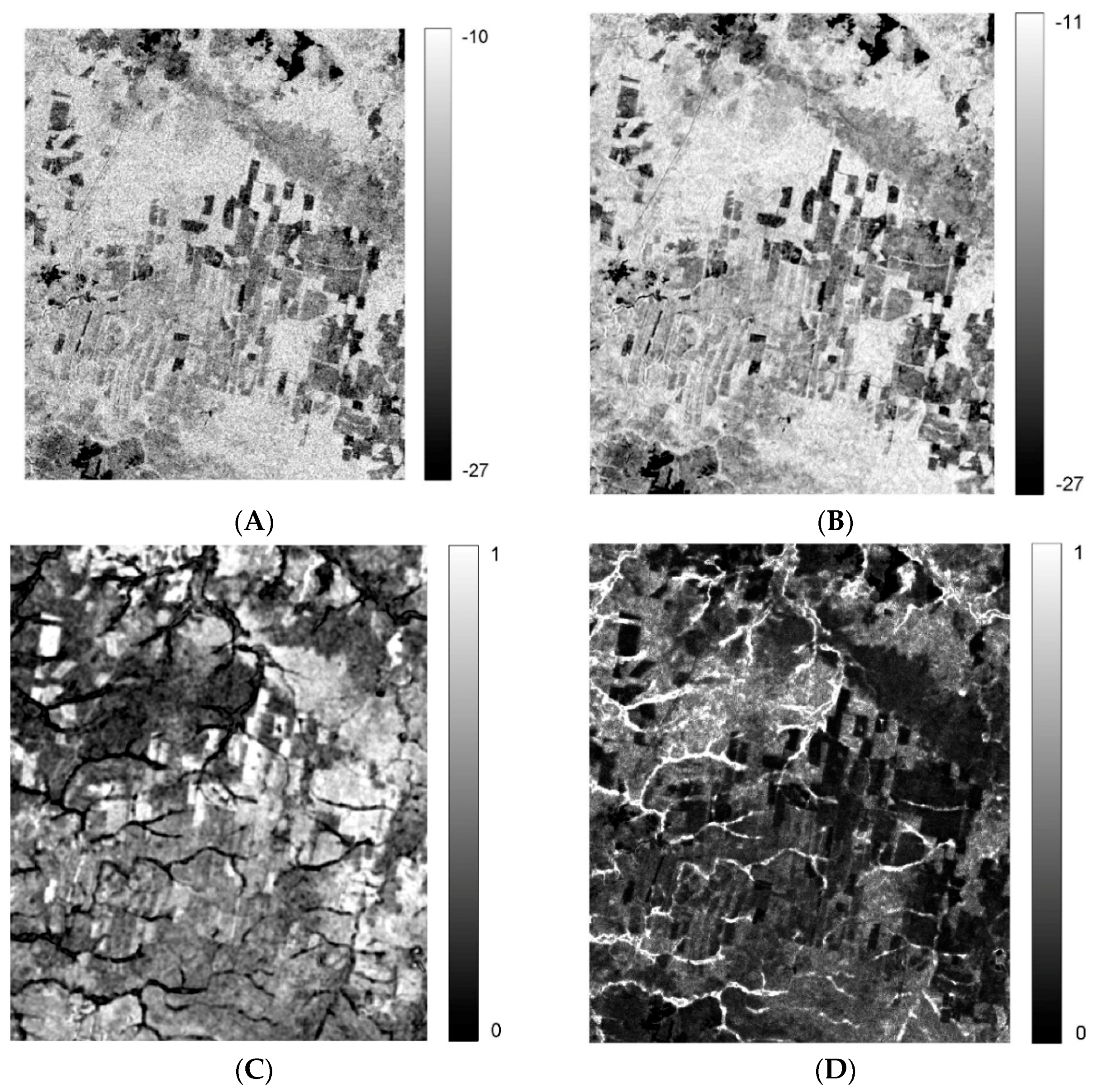
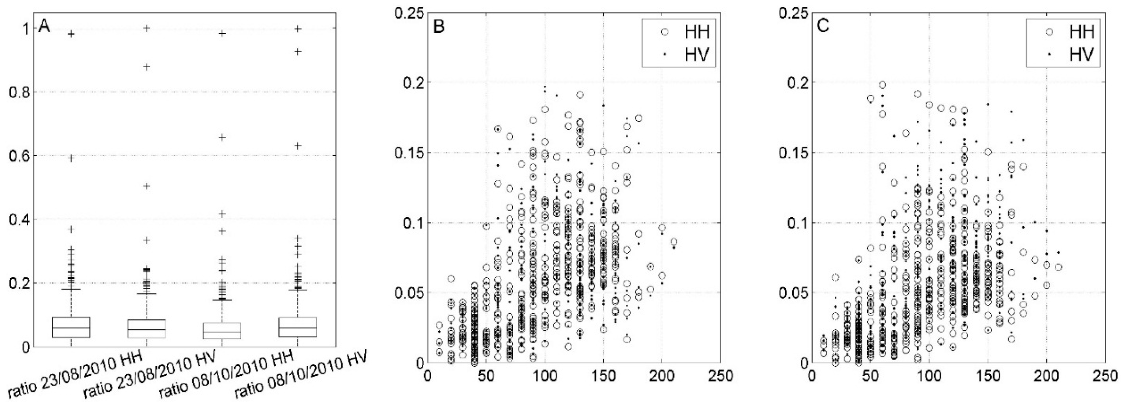
3.2. SAR Data Processing and Data Selection

The first pre-processing steps of SAR data included data calibration and multi-looking. In order to obtain data with squared pixels of approximately 50 m spatial resolution, the following multi-looking factors (range x azimuth) were used: FBS mode 6 × 15, FBD mode 3 × 15. Thereafter, the SAR backscattering coefficient was calculated as γ°, which includes a correction of the backscatter for the local incidence angle θ_i [84]:

$${\mathsf{\gamma }}^0={\mathsf{\sigma }}^0\frac{A_{flat}}{A_{slope}}{\left(\frac{\cos \left(\mathsf{\theta }\right)}{cos\left({\mathsf{\theta }}_i\right)}\right)}^n$$

(7)

where ${\mathsf{\sigma }}^0$is the backscattering coefficient and $\mathsf{\theta }$ the incidence angle measured at mid-swathe (34.3°). $A_{flat}$ and $A_{slope}$ represent the local and the true pixel area, respectively. The cosine of the local incidence angle ${\mathsf{\theta }}_i$ corrects the radiometry of backscatter for local slopes and converts the data from σ° to ${\mathsf{\gamma }}^0$. This correction is known as a topographic normalization based on the local incidence angle and pixel area. In total eight backscatter images acquired in FBD mode were generated. The data selection was based on the recommendations from previous studies, in which it was reported that the backscatter data acquired during summer and autumn were superior to the winter acquisitions with regards to the AGB/GSV retrieval [31,85,86].

To reduce the speckle effect in the backscatter data, a filtering approach was implemented. The method was based on a multi-temporal speckle filtering calculated according to [87]:

$$J_k\left(x,y\right)=\frac{\langle I_k\rangle }{N}{\displaystyle \sum }_{i=1}^N\frac{I_i\left(x,y\right)}{I_i}$$

(8)

where I is the local mean value of pixels in a window with a center at (x, y) in image I, k = 1,..,N and N represents the number of multi-temporal images, with intensity at position (x, y) in the k image—$I_i\left(x,y\right). J_k$ filters uncorrelated speckle between the images. In this study, N was equal to 8 for filtering of intensity images and window size was 5 × 5. No larger filtering window size was used because already large multi-looking factors were implemented.

The coherence images were calculated according to [88]:

$$\mathsf{\gamma }=\left|\mathsf{\gamma }\right|{\mathrm{e}}^{\mathrm{j}\mathsf{\varphi }}=\frac{\mathrm{E}\left\{g_1{g^{*}}_{2 }\right\}}{\sqrt{\mathrm{E}\{{\left|g_1\right|}^2\}E\{{\left|g_2\right|}^2\}}}$$

(9)

where ф is the phase and E{} represents expected value.

Coherence measures the degree of correlation between two SAR images and takes values between 0 for total decorrelation and 1 for perfect correlation. Data processing consisted of co-registration at sub-pixel level (less than 0.05 pixel), common range and azimuth band filtering, and interferogram calculation and flattening. Coherence was estimated by spatial averaging within a two-dimensional window. In this study an adaptive estimation window was used with a window size between 3 × 3 and 5 × 5. A larger window size was used in the areas of low coherence in order to reduce the coherence bias. The resulting coherence was computed using the same number of looks as in the case of backscatter data (FBS mode 6 × 15, FBD mode 3 × 15 in range, and azimuth). This number of looks significantly reduced the coherence overestimation for low coherence values, as described in [89]. Therefore, the coherence bias was calculated to be close to zero (for coherence equal to 0 the values were ~0.002). The coherence was generated for 19 SLC pairs (Table 3). As a master image the image acquired in 2010 was used, additionally coherence for data acquired in 2011 was calculated. The perpendicular baselines B_n were between 224 and 3829 m and thus shorter than the critical baselines: 14.7 and 7.3 km for the FBS and FBD modes, respectively. Five coherence images were considered for the AGB retrieval. The latter were selected according to the stable weather and environmental conditions during the data acquisition [50] and a simple visual interpretation. To avoid coherence variability due to topography, slopes greater than 5° were masked out (mainly riverside areas). The mask was implemented to all SAR products used for AGB estimation. The SAR images were geocoded and normalized using the Shuttle Radar Topography Mission (SRTM) 90 m digital elevation model version 4.1 [90,91]. The SAR pre-processing was performed with the GAMMA Interferometric SAR Processor [92]. The backscatter data were geocoded using the bicubic-log spline resampling method while the coherence data were processed with the bicubic spline interpolation approach. The final spatial resolution of the SAR products was 50 m.

Table 3. Summary of coherence images generated for the test site.

PALSAR Data	Perpendicular Baseline |Bn| (m)	Temporal Baseline Bt (days)
5 January 2010 & 20 February 2010	789	46
23 August 2010 & 8 October 2010	461	46
8 October 2010 & 23 November 2010	224	46
28 December 2006 & 5 January 2010	2390	1104
12 February 2007 & 5 January 2010	1111	1058
12 February 2007 & 20 February 2010	1899	1104
31 December 2007 & 5 January 2010	1086	736
31 December 2007 & 20 February 2010	297	782
15 February 2008 & 5 January 2010	2190	690
15 February 2008 & 20 February 2010	1401	736
2 January 2009 & 5 January 2010	3041	368
2 January 2009 & 20 February 2010	3829	414
17 February 2009 & 5 January 2010	2339	322
17 February 2009 & 20 February 2010	3126	368
5 January 2010 & 8 January 2011	2978	368
20 February 2010 & 8 January 2011	2190	322
5 January 2010 & 23 February 2011	3780	414
20 February 2010 & 23 February 2011	2992	368
8 January 2011 & 23 February 2011	803	46

Table 3. Summary of coherence images generated for the test site.

PALSAR Data	Perpendicular Baseline |Bn| (m)	Temporal Baseline Bt (days)
5 January 2010 & 20 February 2010	789	46
23 August 2010 & 8 October 2010	461	46
8 October 2010 & 23 November 2010	224	46
28 December 2006 & 5 January 2010	2390	1104
12 February 2007 & 5 January 2010	1111	1058
12 February 2007 & 20 February 2010	1899	1104
31 December 2007 & 5 January 2010	1086	736
31 December 2007 & 20 February 2010	297	782
15 February 2008 & 5 January 2010	2190	690
15 February 2008 & 20 February 2010	1401	736
2 January 2009 & 5 January 2010	3041	368
2 January 2009 & 20 February 2010	3829	414
17 February 2009 & 5 January 2010	2339	322
17 February 2009 & 20 February 2010	3126	368
5 January 2010 & 8 January 2011	2978	368
20 February 2010 & 8 January 2011	2190	322
5 January 2010 & 23 February 2011	3780	414
20 February 2010 & 23 February 2011	2992	368
8 January 2011 & 23 February 2011	803	46

In addition to the backscatter and coherence data, the normalized ratio of the backscatter in linear scale and coherence, R_n, was calculated:

$$R_n=\frac{\raisebox{1ex}{${\mathsf{\gamma }}^0$}\!\left/ \!\raisebox{-1ex}{$\mathsf{\gamma }$}\right.-min\left(\raisebox{1ex}{${\mathsf{\gamma }}^0$}\!\left/ \!\raisebox{-1ex}{$\mathsf{\gamma }$}\right.\right)}{max\left(\raisebox{1ex}{${\mathsf{\gamma }}^0$}\!\left/ \!\raisebox{-1ex}{$\mathsf{\gamma }$}\right.\right)-min\left(\raisebox{1ex}{${\mathsf{\gamma }}^0$}\!\left/ \!\raisebox{-1ex}{$\mathsf{\gamma }$}\right.\right)}.$$

(10)

The rationale behind the ratio calculation is purely statistical. The ratio was introduced to enhance the backscatter relation to AGB and to reduce the number of potential outliers influencing the AGB retrieval error. In this approach, coherence γ values are considered as weighting factors for the backscatter γ° (linear scale) and strengthen the response over forested areas. The ratio calculation was performed using a reference coherence image with a temporal baseline of 46 days. The SLC data for the coherence calculation were acquired in winter 2010, namely on 5 January 2010 and 20 February 2010. This coherence was selected due to the highest dynamic range of coherence values resulted from optimal and similar environmental conditions during the data acquisition, as well as the short perpendicular baseline B_n. The resulting ratio values over forested areas are relatively high compared to the values over non-forested and sparsely forested areas. For example, a value of 0.16 of backscatter on a linear scale with a corresponding coherence value of 0.2 (dense forest) is approximately 0.8, whereas a backscatter value of 0.07 with a coherence value of 0.6 (non-forest) is approximately 0.1. In order to adjust the ratio values to a single scale, the values were normalized and ranged from 0 to 1. A normalized ratio between available backscatter data (in linear scale) acquired on 23 August 2010 and 8 October 2010 in both polarizations and the coherence between acquisitions taken in 2010 (5 January and 20 February) were calculated. The resulting range of calculated values is illustrated by box plots (Figure 4, plot A).

On each box the central mark is the median, the edges of the box are the 25th and 75th percentiles, and the whiskers extend to the extreme values. Most of the values varied from 0 to approximately 0.2 show an almost linear relationship up to approximately 60 t·ha⁻¹ and a non-linear relationship for higher AGB values (Figure 4B,C). The values close to the upper boundary represented small heterogeneous stands in the forest inventory data (<8 ha).

Figure 4. (A) presents box plots for four calculated ratios between backscatter images (acquired on 23 August 2010 and 8 October 2010) and coherence acquired in winter 2010 (5 January and 20 February); (B) and (C) present the ratio as a function of aboveground biomass (AGB).

Figure 4. (A) presents box plots for four calculated ratios between backscatter images (acquired on 23 August 2010 and 8 October 2010) and coherence acquired in winter 2010 (5 January and 20 February); (B) and (C) present the ratio as a function of aboveground biomass (AGB).

In total, 13 SAR products were selected for AGB retrieval. The examples of the generated SAR products are presented in Figure 5.

Figure 5. Subset of SAR products used for AGB retrieval. (A): backscatter data acquired on 23 August 2010 in HV polarization in dB; (B): filtered backscatter image in dB; (C): coherence between 5 January 2010 and 20 February 2010; (D): normalized ratio between acquired on 23 August 2010 in HV polarization and coherence (5 January & 20 February 2010).

Figure 5. Subset of SAR products used for AGB retrieval. (A): backscatter data acquired on 23 August 2010 in HV polarization in dB; (B): filtered backscatter image in dB; (C): coherence between 5 January 2010 and 20 February 2010; (D): normalized ratio between acquired on 23 August 2010 in HV polarization and coherence (5 January & 20 February 2010).

3.3. AGB Retrieval Models

In this study, two non-parametric data fusion machine learning algorithms were considered: maximum entropy (MaxEnt) and Random Forests. In both cases the updated forest inventory was used as the response data. The model’s training was done on 90% of the sample size (577 samples), whereas 10% was used for independent validation (64 samples). For the selection of training and validation data, a stratified sampling was implemented. Only 10% of the response data was used for the independent validation as the mentioned algorithms calculate unbiased model error using 25% in the case of MaxEnt and approximately 1/3 in the case of Random Forests of the data randomly excluded from the training data.

The first approach was a model based on the MaxEnt algorithm. The model was run using the MaxEnt program for maximum entropy modeling version 3.3.3 k (under Java Runtime Environment). The MaxEnt is an exponential model that can be compared with the generalized linear (GLM) and generalized additive (GAM) models. The concept of the method is to estimate the probability distribution of maximum entropy constrained by a set of remote sensing variables. Through numerous iterations, the weights of these variables are adjusted to maximize the average sample likelihood (training gain). The weights are then used to estimate the distribution over the whole space for each of the AGB classes. In this study, AGB reference data were divided into seven AGB classes, in t·ha⁻¹: 0–40, 40–60, 60–80, 80–100, 100–120, 120–140, and >140. The values were grouped such that each class could be represented equally in terms of occurrences. The classes’ representation is illustrated as a histogram (Figure 6).

Figure 6. Number of measurements in selected AGB class.

Figure 6. Number of measurements in selected AGB class.

Then, the AGB value was calculated for each pixel using the maximum probability weighted average [64]:

$$\widehat{AGB}=\frac{{{\displaystyle \sum }}_{i=1}^N{\mathrm{P}}_i^{n}AG{B}_i}{{{\displaystyle \sum }}_{i=1}^N{P}_i^n}$$

(11)

where i refers to the class number, $P_i$ is the MaxEnt probability, $AG{B}_i$ is the estimated average biomass range, and $\widehat{AGB}$ is the predicted value of AGB for each pixel.

As an input for the MaxEnt algorithm, all available variables were used and two groups of data were distinguished. The first one contained unfiltered data, whereas the second one was with backscatter data filtered according to Equation (8).

In the MaxEnt program the resampling of the data for each replication is done by bootstrapping, whereas the jackknife tests are used for calculation of variable contribution. The jackknife tests are generated using regularized gain and AUC. The jackknife test is used in two cases: withhold one predictor and refit model and withhold all predictors but one and refit the model. To determine the variable percent contribution, in each iteration of the training algorithm the increase in regularized gain was added to the contribution of the corresponding variable, or subtracted from it if the resulted value was negative. At the end the values were converted to percentages.

The second approach was based on a supervised Random Forests^® regression approach, available as the randomForest package in the R software [93]. It is an ensemble learning method that operates by constructing a large number of trees by randomly selecting the predictors and then calculating a mean prediction from all individual regression trees. Each tree is constructed using a different randomly permuted sample from the input dataset. One-third of the data are left out of the bootstrap sample and not used in the construction of the tree. This sample is called out-off-bag (OOB) and is used to obtain an unbiased estimate for the retrieval error, OOB error.

The randomForest package also provides measures for evaluating the importance of the different predictors in the model development. In this study, we used the measure that is computed from permuting OOB data and permuting each predictor variable for each tree. The difference between the OOB MSE and predictor MSE are then averaged over all trees, and normalized by the standard deviation of the differences.

In order to evaluate the accuracy and performance of the implemented models, the following quantitative measures were considered for the independent validation:

a. root mean square error (RMSE) is defined as:

$$RMSE=\sqrt{\frac{{{\displaystyle \sum }}_{i=1}^n{\left(AG{B}_{ref\left(i\right)}-{\widehat{AGB}}_{i }\right)}^2}{n}}$$

(12)

where $AG{B}_{ref\left(i\right)}$ represents AGB reference value for stand i, ${\widehat{AGB}}_{i }$predicted AGB and n a number of AGB observations.

b. corrected root-mean-square error ($rRMS{E}_{cor}$) is defined as:

$$rRMS{E}_{cor}=\sqrt{RMS{E}_{Sat}^2-RMS{E}_{Ref}^2}$$

(13)

where $RMS{E}_{Sat}$ represents the root mean square error in a satellite-derived estimation of AGB and $RMS{E}_{Ref}$is the root mean square error in the forest inventory data. According to the manual on forest inventory and planning in Russian forests, the maximum error of GSV is expected to be 15% [94]. This value was also considered in the AGB estimation because GSV is the main component of AGB. According to [95], GSV constitutes in our test site 73% of AGB.

Additionally, relative RMSEs were calculated by dividing the RMSEs by the mean AGB and multiplying by 100%.

c. bias is defined as the mean of estimation error:

$$bias=\frac{{{\displaystyle \sum }}_{i=1}^n\left( {\widehat{AGB}}_i-AG{B}_{ref\left(i\right)}\right)}{n}$$

(14)

where positive values of bias expresses overestimation, and negative values underestimation.

The models’ predictive performance was evaluated using pseudo R-squared (1-MSE/variance) [93] in the case of the Random Forests and an area under receiver operating characteristic curves (AUC) [96] in the case of the MaxEnt. The parameters were generated using the models’ testing samples.

4. Retrieval Results

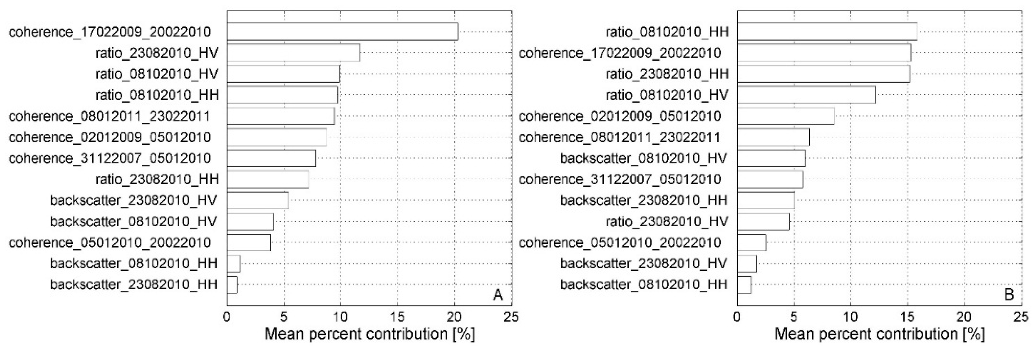
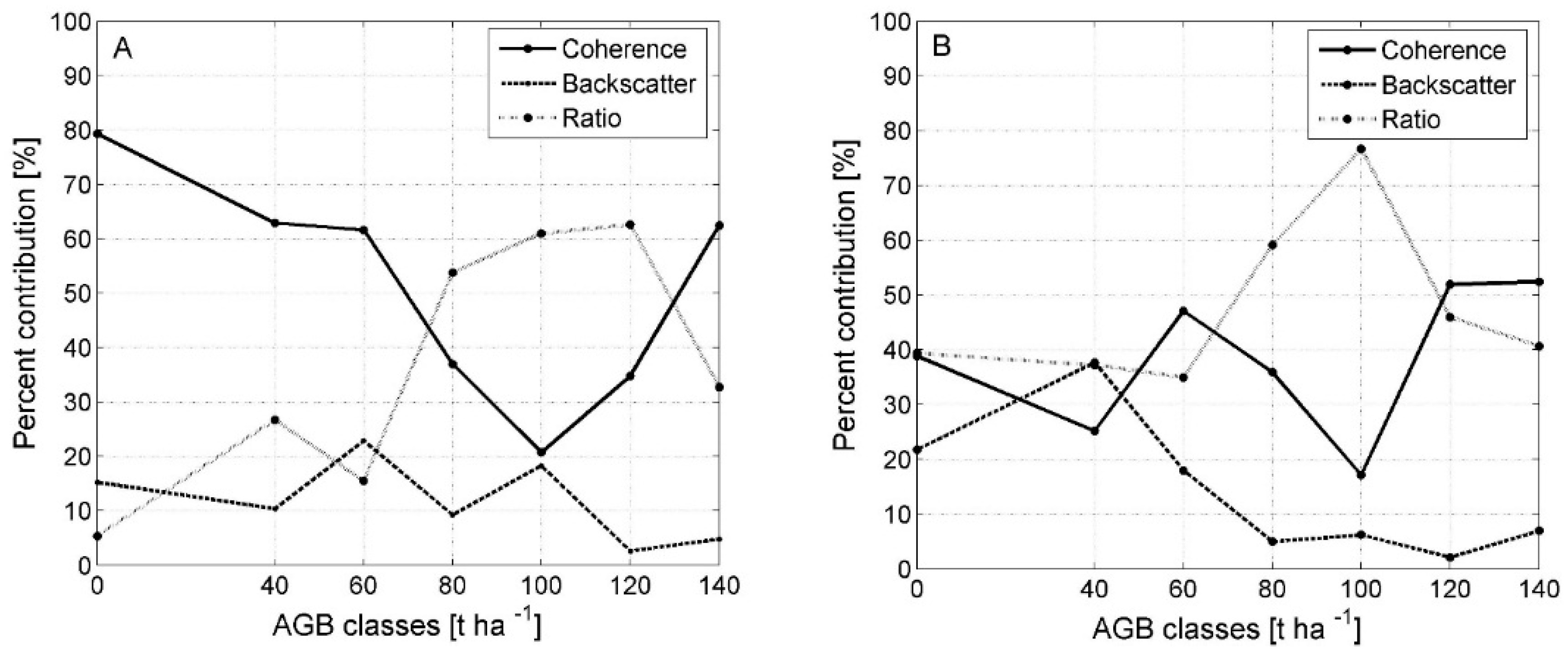
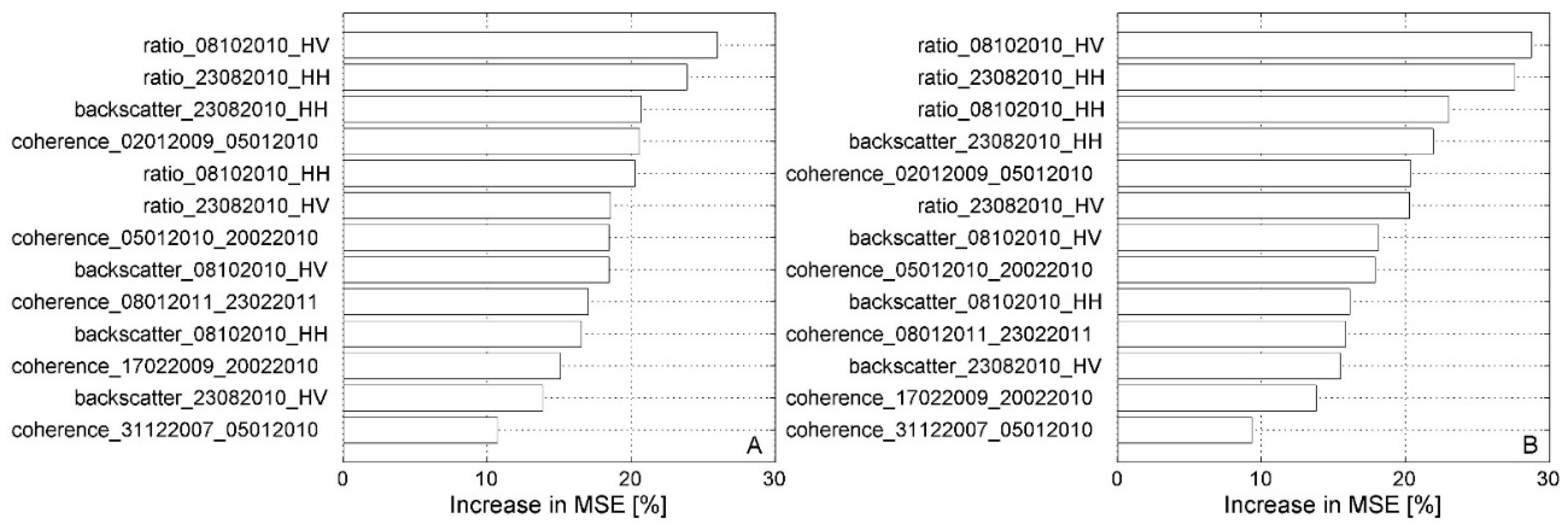
4.1. MaxEnt Performance

As an output of MaxEnt seven continuous probability distribution maps with pixel values from 0 to 1 were obtained, where 1 is a high predicted probability of being classified to a specified AGB class. The probability values were then used to calculate the final AGB map according to Equation (11).

To assess the MaxEnt algorithm performance, AUC was calculated by bootstrapping 25% of the training data. The AUC was computed for each AGB class (Figure 7).

The AUC values are higher than 0.7, which shows that the model performed well. Only in the case of filtered data or the 60–80 t·ha⁻¹ AGB class was the AUC was lower than 0.6. The highest predictive power of the model was observed for the high and the low AGB ranges. The mean AUC for all AGB classes was calculated to be 0.76 and 0.77 for unfiltered and filtered datasets, respectively.

To assess the importance of the predictors, the variable percent of contribution was calculated. A high value indicates that the model depends more on that variable (Figure 8A,B).

Figure 7. Evaluation of MaxEnt model performance using Area Under the Receiver Operator Curve (AUC) for testing dataset (A) with unfiltered and (B) with filtered backscatter data; aboveground biomass (AGB) classes 0: 0–40, 40: 40–60, 60: 60–80, 80: 80–100, 100: 100–120, 120: 120–140, 140: >140 t·ha⁻¹.

Figure 7. Evaluation of MaxEnt model performance using Area Under the Receiver Operator Curve (AUC) for testing dataset (A) with unfiltered and (B) with filtered backscatter data; aboveground biomass (AGB) classes 0: 0–40, 40: 40–60, 60: 60–80, 80: 80–100, 100: 100–120, 120: 120–140, 140: >140 t·ha⁻¹.

Figure 8. Predictor importance presented as percent contribution (A) dataset with unfiltered and (B) with filtered backscatter data.

Figure 8. Predictor importance presented as percent contribution (A) dataset with unfiltered and (B) with filtered backscatter data.

In the case of the dataset with the unfiltered backscatter, the variable that mostly decreased model performance when it was omitted was coherence between data acquired on 17 February 2009 and 20 February 2010. For the filtered dataset, it was the ratio of backscatter in HH polarization acquired on 8 October 2010. Therefore, the coherence and normalized ratio appear to contain the most information that is not present in the other variables. The backscatter acquired on 23 August 2010 in HH and on 8 October 2010 in HH polarization seem to be of less importance for AGB prediction.

The variable importance was also analyzed per AGB class. To better illustrate how the variable contribution changes among the seven AGB classes, the data were distinguished between coherence, backscatter, and normalized ratio (Figure 9).

Figure 9. Coherence, backscatter, and normalized ratio contributions versus AGB classes. (A) Dataset with unfiltered or (B) filtered backscatter data. Class 0 represents AGB values from 0 to 40, 40: 40–60, 60: 60–80, 80: 80–100, 100: 100–120, 120: 120–140, 140: >140 t·ha⁻¹.

Figure 9. Coherence, backscatter, and normalized ratio contributions versus AGB classes. (A) Dataset with unfiltered or (B) filtered backscatter data. Class 0 represents AGB values from 0 to 40, 40: 40–60, 60: 60–80, 80: 80–100, 100: 100–120, 120: 120–140, 140: >140 t·ha⁻¹.

Figure 9 confirms with a mean percent contribution value of 51.2% that in the case of unfiltered data the most important variables were coherence data. The data were the most important in four AGB classes: 0–40, 40–60, 60–80, and >140 t·ha⁻¹. The mean percent contribution for the ratio products was 36.8% and for the backscatter products was 12%. Therefore, the backscatter seems to provide the least information for MaxEnt. When the filtered data were used, the most important group of data was the ratio layers, with a mean percent contribution of 47.7%. The data were the most important in two classes, i.e., AGB classes 80–100 and 100–120 t·ha⁻¹. The second most important type of data was the coherence products, with a mean percent contribution of 38.3%. The data contributed most to the AGB retrieval for three AGB classes 60–80, 120–140, and >140 t·ha⁻¹. The backscatter data provided the least information for the retrieval. The mean percent contribution was 13.9%. In both plots the rise of the ratio importance is related to the decrease of the influence of the backscatter and coherence.

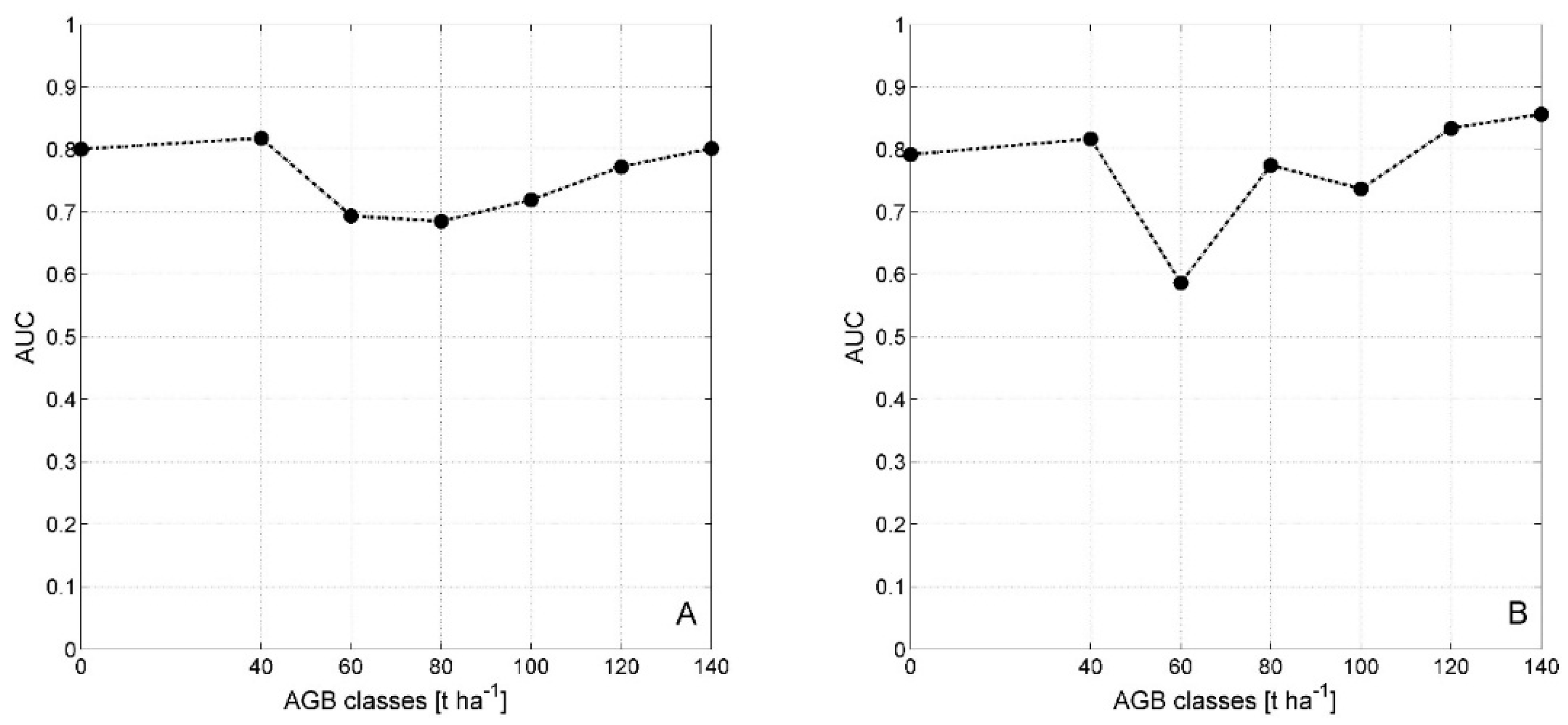
4.2. Random Forests Performance

The higher percent of variance explained was calculated for the dataset with filtered backscatter, the value of the pseudo R-squared was 38.4%. In the case of the unfiltered dataset the pseudo R-squared was 36.4%. The values were calculated based on the testing sample (OOB sample). Overall, the Random Forests predictor importance ranking (Figure 10) revealed only small differences between the datasets with unfiltered and filtered backscatter data. The ranking showed that of the 13 predictors the normalized ratio between the backscatter in HV polarization acquired on 8 October 2010 and coherence (5 January & 20 February 2010) was the most important for the retrieval of AGB with values of 26% and 28.7% for the unfiltered and filtered datasets, respectively. The mean value of the increase in MSE in the case of all ratio products was 22.2% and 24.9%.

The second most important data group in the case of the both datasets was backscatter products. The mean value of the increase in MSE was 17.4% and 17.9%. Random Forests suggested that coherence products had the smallest influence on AGB retrieval with a mean value of 16.4% and 15.4% for unfiltered and filtered datasets, respectively.

Figure 10. Predictor importance presented as increase in MSE for (A) unfiltered dataset and (B) dataset with filtered backscatter data.

Figure 10. Predictor importance presented as increase in MSE for (A) unfiltered dataset and (B) dataset with filtered backscatter data.

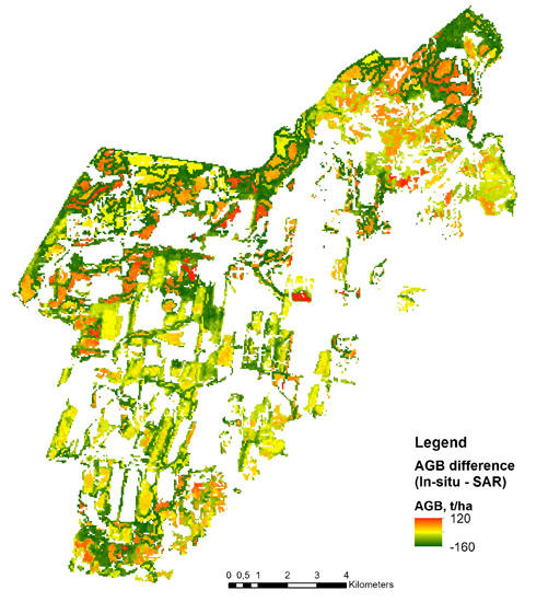
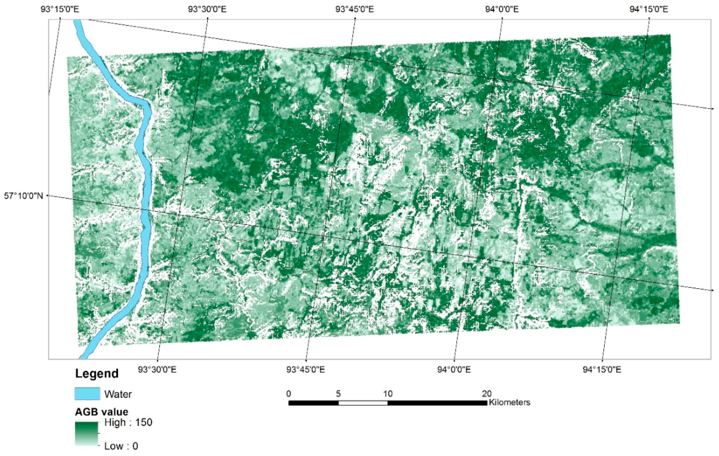
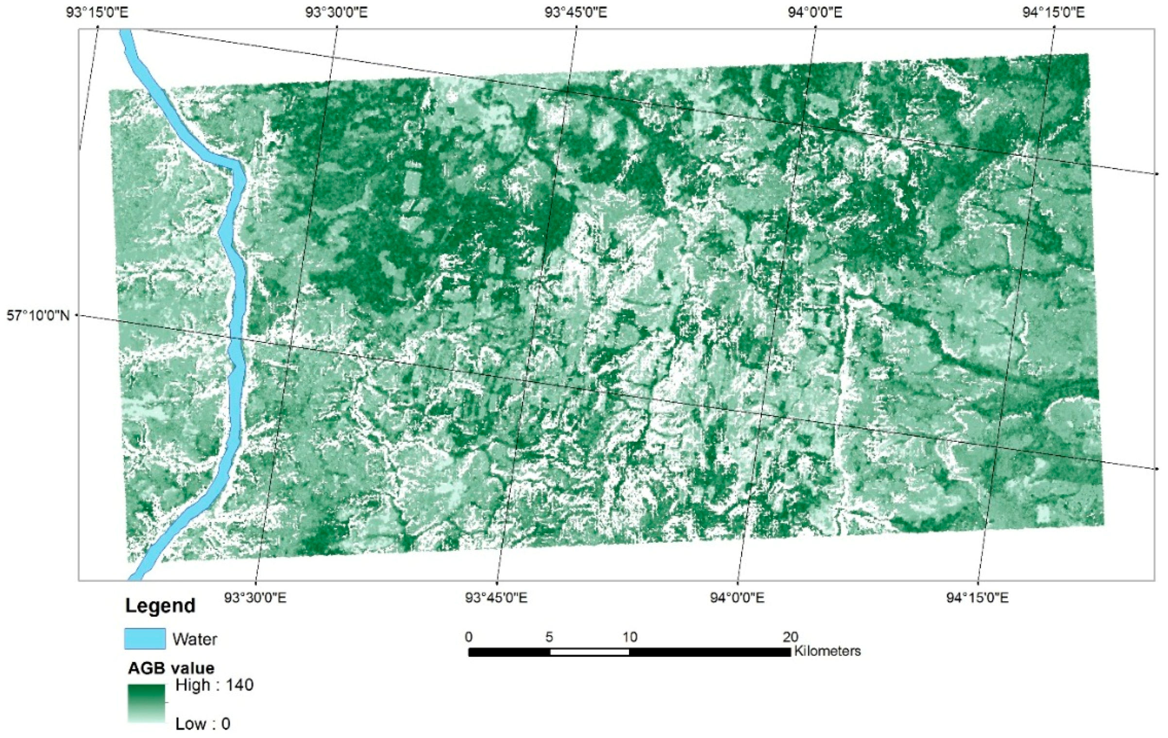
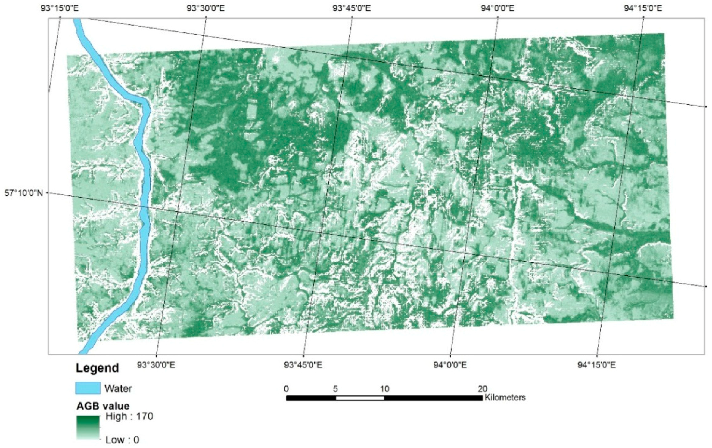
4.3. AGB Mapping Results

Figure 11, Figure 12, Figure 13 and Figure 14 show SAR-derived AGB maps with a spatial resolution of 50 m. Each map presents AGB retrieval results expressed in t·ha⁻¹. The first two maps show AGB values derived by the MaxEnt algorithm; the other two are by the Random Forests. Examining the results with a simple visual interpretation, it can be noticed that the maps differ taking into account the spatial variability of AGB values. In the case of the AGB maps generated by MaxEnt, the values seem to be more heterogonous both in high and low biomass ranges.

The range and the mean value of the retrieved AGB for each map are given in Table 4.

Table 4. Range of derived AGB.

Method	MaxEnt Unfiltered Dataset	Random Forests Unfiltered Dataset	Maxent Filtered Dataset	Random Forests Filtered Dataset
Range t·ha−1	0–140	0–160	0–150	0–170
Mean AGB t ha−1	87	95	89	97

Table 4. Range of derived AGB.

Method	MaxEnt Unfiltered Dataset	Random Forests Unfiltered Dataset	Maxent Filtered Dataset	Random Forests Filtered Dataset
Range t·ha−1	0–140	0–160	0–150	0–170
Mean AGB t ha−1	87	95	89	97

In the case of the MaxEnt algorithm, the AGB ranged from 0 to 140 (150 t·ha⁻¹), whereas the values computed by the Random Forests were higher by 10 t·ha⁻¹. The mean values derived by MaxEnt were lower than 90 t·ha⁻¹ and in the case of Random Forests greater than 95 t·ha⁻¹.

Figure 11. AGB map generated using the MaxEnt algorithm and a dataset with unfiltered backscatter data.

Figure 11. AGB map generated using the MaxEnt algorithm and a dataset with unfiltered backscatter data.

Figure 12. AGB map generated using the MaxEnt algorithm and a dataset with filtered backscatter data.

Figure 12. AGB map generated using the MaxEnt algorithm and a dataset with filtered backscatter data.

Figure 13. AGB map generated using the Random Forests algorithm and a dataset with unfiltered backscatter data.

Figure 13. AGB map generated using the Random Forests algorithm and a dataset with unfiltered backscatter data.

To better observe the differences in spatial distribution, the difference maps between updated forest inventory (in situ data) and SAR-derived AGB were calculated (Figure 15). Green represents overestimation, whereas red is underestimation. In yellow are the AGB values estimated correctly.

In general, there are almost no differences between maps generated using unfiltered and filtered datasets. In the case of MaxEnt, the retrieved AGB values are displayed in green, which means overestimation. The Random Forests tends to underestimate. The AGB values are displayed in red and orange. In both cases, the overestimation can be seen on the borders of the stands. The underestimation is observed for stands with high AGB values.

Figure 14. AGB map generated using the Random Forests algorithm and a dataset with filtered backscatter data.

Figure 14. AGB map generated using the Random Forests algorithm and a dataset with filtered backscatter data.

Figure 15. AGB difference maps between updated forest inventory (in situ) and SAR-derived AGB. (A) MaxEnt model—unfiltered data; (B) Random Forests—unfiltered data; (C) MaxEnt model with filtered backscatter; (D) Random Forests with filtered backscatter.

Figure 15. AGB difference maps between updated forest inventory (in situ) and SAR-derived AGB. (A) MaxEnt model—unfiltered data; (B) Random Forests—unfiltered data; (C) MaxEnt model with filtered backscatter; (D) Random Forests with filtered backscatter.

4.4. Validation

Table 5 summarizes the accuracies of the MaxEnt and the Random Forests AGB retrieval when using backscatter data (filtered and unfiltered), coherence images, and normalized ratio products. The corrected RMSE and relative corrected RMSE were calculated for a training sample and an independent sample.

Table 5. Validation of AGB retrieval results. RMSE values are given for training and validation samples (training/validation).

Model	Dataset	RMSEcor (t·ha−1)	rRMSEcor (%)	Bias (t·ha−1)
MaxEnt	Unfiltered	33.3/36.4	34.3/39.5	12.0/5.2
	Filtered	28.7/35.8	29.6/38.8	6.9/4.3
Random Forests	Unfiltered	21.6/35.4	22.3/38.4	3.2/−4.4
	Filtered	21.3/35.0	22.0/36.9	0.9/−4.5

Table 5. Validation of AGB retrieval results. RMSE values are given for training and validation samples (training/validation).

Model	Dataset	RMSEcor (t·ha−1)	rRMSEcor (%)	Bias (t·ha−1)
MaxEnt	Unfiltered	33.3/36.4	34.3/39.5	12.0/5.2
	Filtered	28.7/35.8	29.6/38.8	6.9/4.3
Random Forests	Unfiltered	21.6/35.4	22.3/38.4	3.2/−4.4
	Filtered	21.3/35.0	22.0/36.9	0.9/−4.5

In the case of MaxEnt, the corrected RMSE was 36.4 t·ha⁻¹ (33.3 t·ha⁻¹ for the training sample) and 28.7 t·ha⁻¹ (35.8 t·ha⁻¹ for the training sample) for unfiltered and filtered datasets, respectively. Overall, the estimation error of 39.5% (34.3% for training sample) was calculated for an unfiltered dataset and 38.8% (29.6% for the training sample) for a dataset with filtered backscatter data. The bias of 5.2 t·ha⁻¹ (12 t·ha⁻¹ for the training sample) was calculated in the case of unfiltered data and of 4.3 t·ha⁻¹ (6.9 t·ha⁻¹ for the training sample) in the case of the dataset with filtered backscatter data.

The Random Forests results show similar estimation error. The corrected RMSE was 35.4 t·ha⁻¹ (21.6 t·ha⁻¹ for training sample) and 35.0 t·ha⁻¹ (21.3 t·ha⁻¹ for training sample) for unfiltered and filtered datasets, respectively. The relative corrected RMSEs of 38.4% (22.3% for the training sample) in the case of unfiltered datasets and of 36.9% (22.0% for the training sample) were calculated. The bias of −4.4 t·ha⁻¹ (3.2 t·ha⁻¹ for the training sample) and of −4.5 t·ha⁻¹ (0.9 t·ha⁻¹ for the training sample) was calculated in the case of unfiltered and filtered data, respectively.

It should be noted that a difference of more than 10 t·ha⁻¹ in the case of the Random Forests between corrected RMSE calculated using training and validation datasets could result from the small size of validation sample.

5. Discussion

In general, the MaxEnt machine learning algorithm as well as the Random Forests regression approach provided good AGB retrieval results compared to previous studies [51,52,55,58,60]. The reported analyses also used ALOS PALSAR L-band data for AGB/GSV retrieval over Siberian boreal forests. The researchers reported RMSEs between 33 and 87 m³·ha⁻¹ and 55 t·ha⁻¹ at the coarser scales, and 36.4 t·ha⁻¹ at 0.25 ha scale. Those results are similar to or worse than those derived in this study. The results presented in this paper showed that a relatively high estimation accuracy (down to 30%) can be obtained at a local scale. The AGB estimation showed only slightly better results when a dataset with filtered backscatter intensity was used.

When the model performance is taken into account, the MaxEnt performed better than the Random Forests. The area under the receiver operator curve (AUC) was higher than 0.7, except the AGB range from 60 to 80 t·ha⁻¹, whereas Random Forests reached an R² of 38.4%. MaxEnt generated AGB maps with dominantly overestimated AGB values, whereas Random Forests provided slightly underestimated values. The range of derived AGB values was underestimated but similar and differs by 10 t·ha⁻¹ between the applied models. The mean AGB provided by Random Forests was comparable to the reference AGB mean. MaxEnt showed an underestimation of approximately 10 t·ha⁻¹. The estimation bias was lower in the case of Random Forests.

MaxEnt and Random Forests provided measures for evaluating the importance of the predictors used in the model construction. The algorithms showed no agreement between derived variable rankings. In the case of MaxEnt, the coherence together with the ratio products were the most important for model construction, whereas ratio and backscatter products provided the most information in the case of modeling with Random Forests. In both cases, the ratio products seem to provide important information for AGB retrieval. Within the data groups, in the case of the MaxEnt the most important variables were the coherence between images acquired on 17 February 2009 and 20 February 2010, the normalized ratio between the backscatter from 23 August 2010 in HV and coherence, the backscatter from 23 August 2010 in HV polarization for unfiltered dataset. For filtered dataset, the most important variables within the data groups were the normalized ratio between the backscatter from 8 October 2010 in HH polarization and coherence, the coherence between images acquired on 17 February 2009 and 20 February 2010, and the backscatter image acquired on 23 August 2010 in HV polarization. In the case of Random Forests, the most important variables were the normalized ratio between the backscatter acquired on 8 October 2010 in HV polarization and coherence, the backscatter acquired on 23 August 2010 in HH polarization, and the coherence between images from 2 January 2009 and 5 January 2010 for both unfiltered and filtered datasets. The coherence images generated with the temporal baseline (B_t) greater than 46 days were superior to those derived with shorter B_t.

6. Conclusions

In this study we have demonstrated the feasibility of synergistic usage of backscatter and coherence for aboveground biomass (AGB) retrieval for boreal forests in Siberia at a local scale of 0.25 ha. This research was focused on the further exploitation of SAR data. The ALOS PALSAR L-band backscatter was combined with coherence, introducing the backscatter–coherence normalized ratio. The latter was developed based on the statistical data analysis. In total 13 variables were used for the AGB estimation. For the AGB retrieval two popular machine learning algorithms were implemented. The MaxEnt and the Random Forests performed well, showing promising AGB estimations and demonstrating the model’s robustness. The corrected RMSEs were between 35.8 and 36.4 t·ha⁻¹ and between 35.8 and 35.0 t·ha⁻¹ for MaxEnt and Random Forests, respectively. The estimation error slightly decreased, by approximately 1%, when the filtered backscatter intensity was used. In this study, the retrieval of AGB using the SAR products was demonstrated only for Siberian unmanaged forests. It is expected that the estimation error over well-managed forests could be further reduced. Estimation improvement is also foreseen at the stand level due to the reduction of the spatial variability in the SAR data. Another issue that could have an influence on the retrieval accuracy is the reference data. Using optical remote sensing data and recommended yield tables and semi-empirical phytomass models in Russian forestry and forest management, the authors updated the old inventory data. Unfortunately, it was not possible to fully validate the obtained values in the field, hence the error in the reference data was only partially known.

The models provided different variable importance rankings. However, in both cases the normalized ratio products seem to contain important information for the model development. The coherence data were the most important in the low and high AGB ranges, whereas the ratio was most important for middle to high AGB ranges. Thus, a strategy of using different datasets for estimation of low, medium, and high AGB values could further increase biomass retrieval accuracy. It was observed that the backscatter data increased their contribution in the model construction after filtering. In terms of the retrieved AGB values, the Random Forests algorithm provided AGB mean estimation almost the same as the reference value. MaxEnt provided slightly overestimated AGB values, whereas Random Forests tended to underestimate the AGB values.

The MaxEnt and Random Forests machine learning algorithms demonstrated their potential use for forestry applications, especially for estimations in remote areas. Often no information about AGB is available in those regions. The models could be used to provide AGB estimations with relatively low estimation errors. Moreover, the results generated for different time spans could easily be applied for AGB change monitoring, which is very important from the carbon account calculations perspective.

References

1. Houghton, R.A.; Hall, F.; Goetz, S.J. Importance of biomass in the global carbon cycle. J. Geophys. Res. 2009, 114, 1–13. [Google Scholar] [CrossRef]
2. FAO. Global Forest Resources. Assesment 2010. Main report; FAO: Rome, Italy, 2010. [Google Scholar]
3. FAO. State of the World ’s Forests; FAO: Rome, Italy, 2012. [Google Scholar]
4. Pan, Y.; Birdsey, R.A.; Fang, J.; Houghton, R.; Kauppi, P.E.; Kurz, W.A.; Phillips, O.L.; Shvidenko, A.; Lewis, S.L.; Canadell, J.G.; et al. A large and persistent carbon sink in the world’s forests. Science 2011, 333, 988–993. [Google Scholar] [CrossRef] [PubMed]
5. Nilsson, S.; Shvidenko, A.; Jonas, M.; McCallum, I.; Thomson, A.; Balzter, H. Uncertainties of a regional terrestrial biota full carbon account: A systems analysis. Water Air Soil Pollut. Focus 2007, 7, 425–441. [Google Scholar] [CrossRef]
6. Shvidenko, A.Z.; Schepaschenko, D.G.; Vaganov, E.A.; Sukhinin, A.I.; Maksyutov, S.S.; McCallum, I.; Lakyda, I.P. Impact of wildfire in Russia between 1998–2010 on ecosystems and the global carbon budget. Dokl. Earth Sci. 2011, 441, 1678–1682. [Google Scholar] [CrossRef]
7. Kasischke, E.S.; Melack, J.M.; Dobson, M.C. The use of imaging radars for ecological applications—A review. Remote Sens. Environ. 1997, 59, 141–156. [Google Scholar] [CrossRef]
8. Rosenqvist, Å.; Milne, A.; Lucas, R.; Imhoff, M.; Dobson, C. A review of remote sensing technology in support of the Kyoto Protocol. Environ. Sci. Policy 2003, 6, 441–455. [Google Scholar] [CrossRef]
9. Patenaude, G.; Milne, R.; Dawson, T.P. Synthesis of remote sensing approaches for forest carbon estimation: Reporting to the Kyoto Protocol. Environ. Sci. Policy 2005, 8, 161–178. [Google Scholar] [CrossRef]
10. McCallum, I.; Wagner, W.; Schmullius, C.; Shvidenko, A.; Obersteiner, M.; Fritz, S.; Nilsson, S. Satellite-based terrestrial production efficiency modeling. Carbon Balance Manag. 2009, 4. [Google Scholar] [CrossRef] [PubMed]
11. Goetz, S.; Baccini, A.; Laporte, N.; Johns, T.; Walker, W.; Kellndorfer, J.; Houghton, R.; Sun, M. Mapping and monitoring carbon stocks with satellite observations: A comparison of methods. Carbon Balance Manag. 2009, 4, 1–7. [Google Scholar] [CrossRef] [PubMed]
12. Frolking, S.; Palace, M.W.; Clark, D.B.; Chambers, J.Q.; Shugart, H.H.; Hurtt, G.C. Forest disturbance and recovery: A general review in the context of spaceborne remote sensing of impacts on aboveground biomass and canopy structure. J. Geophys. Res. 2009, 114. [Google Scholar] [CrossRef]
13. Thiel, C.; Santoro, M.; Cartus, O.; Thiel, C.; Riedel, T.; Schmullius, C. Perspectives of SAR based forest cover, forest cover change and biomass mapping. In The Kyoto Protocol: Economic Assessments, Implementation Mechanisms, and Policy implications; Vasser, C.P., Ed.; Nova Science Publishers, Inc.: New York, 2009; pp. 13–56. [Google Scholar]
14. Goetz, S.; Dubayah, R. Advances in remote sensing technology and implications for measuring and monitoring forest carbon stocks and change. Carbon Manag. 2011, 2, 231–244. [Google Scholar] [CrossRef]
15. Zolkos, S.G.; Goetz, S.J.; Dubayah, R. A meta-analysis of terrestrial aboveground biomass estimation using lidar remote sensing. Remote Sens. Environ. 2013, 128, 289–298. [Google Scholar] [CrossRef]
16. GOFC-GOLD. A Sourcebook of Methods and Procedures for Monitoring and Reporting Anthropogenic Greenhouse Gas Emissions and Removals Associated with Deforestation, Gains and Losses of Carbon Stocks in Forests Remaining Forests, and Forestation. GOFC-GOLD Report Versio; GOFC-GOLD: Wageningen, The Netherlands, 2014. [Google Scholar]
17. Sader, S.A.; Waide, R.B.; Lawrence, W.T.; Joyce, A.T. Tropical Forest Biomass and Successional Age Class Relationships to a Vegetation Index Derived from Landsat TM Data. Remote Sens. Environ. 1989, 28, 143–156. [Google Scholar] [CrossRef]
18. Wasseige, C.; de Defourny, P. Retrieval of tropical forest structure characteristics from bi-directional reflectance of SPOT images. Remote Sens. Environ. 2002, 83, 362–375. [Google Scholar] [CrossRef]
19. Dong, J.; Kaufmann, R.K.; Myneni, R.B.; Tucker, C.J.; Kauppi, P.E.; Liski, J.; Buermann, W.; Alexeyev, V.; Hughes, M.K. Remote sensing estimates of boreal and temperate forest woody biomass: Carbon pools, sources, and sinks. Remote Sens. Environ. 2003, 84, 393–410. [Google Scholar] [CrossRef]
20. Joshi, C.; Leeuw, J.; de Skidmore, A.K.; Duren, I.C.; van Oosten, H. Remotely sensed estimation of forest canopy density: A comparison of the performance of four methods. Int. J. Appl. Earth Obs. Geoinf. 2006, 8, 84–95. [Google Scholar] [CrossRef]
21. Avitabile, V.; Herold, M.; Henry, M.; Schmullius, C. Mapping biomass with remote sensing: a comparison of methods for the case study of Uganda. Carbon Balance Manag. 2011, 6. [Google Scholar] [CrossRef] [PubMed]
22. Houghton, R.A. Balancing the Global Carbon Budget. Annu. Rev. Earth Planet. Sci. 2007, 35, 313–347. [Google Scholar] [CrossRef]
23. Ji, L.; Wylie, B.K.; Nossov, D.R.; Peterson, B.; Waldrop, M.P.; McFarland, J.W.; Rover, J.; Hollingsworth, T.N. Estimating aboveground biomass in interior Alaska with Landsat data and field measurements. Int. J. Appl. Earth Obs. Geoinf. 2012, 18, 451–461. [Google Scholar] [CrossRef]
24. Lefsky, M.A.; Harding, D.J.; Keller, M.; Cohen, W.B.; Carabajal, C.C.; Del Bom Espirito-Santo, F.; Hunter, M.O.; de Oliveira, R. Estimates of forest canopy height and aboveground biomass using ICESat. Geophys. Res. Lett. 2005, 32, 22–25. [Google Scholar] [CrossRef]
25. Nelson, R.; Ranson, K.J.; Sun, G.; Kimes, D.S.; Kharuk, V.; Montesano, P. Estimating Siberian timber volume using MODIS and ICESat/GLAS. Remote Sens. Environ. 2009, 113, 691–701. [Google Scholar] [CrossRef]
26. Duncanson, L.I.; Niemann, K.O.; Wulder, M.A. Estimating forest canopy height and terrain relief from GLAS waveform metrics. Remote Sens. Environ. 2010, 114, 138–154. [Google Scholar] [CrossRef]
27. Simard, M.; Pinto, N.; Fisher, J.B.; Baccini, A. Mapping forest canopy height globally with spaceborne lidar. J. Geophys. Res. 2011, 116. [Google Scholar] [CrossRef]
28. Khalefa, E.; Smit, I.P.J.; Nickless, A.; Archibald, S.; Comber, A.; Balzter, H. Retrieval of savanna vegetation canopy height from ICESat-GLAS spaceborne LiDAR with terrain correction. IEEE Geosci. Remote Sens. Lett. 2013, 10, 1439–1443. [Google Scholar] [CrossRef]
29. Le Toan, T.; Beaudoin, A.; Riom, J.; Guyon, D. Relating forest biomass to SAR data. IEEE Trans. Geosci. Remote Sens. 1992, 30, 403–411. [Google Scholar] [CrossRef]
30. Kurvonen, L.; Pulliainen, J.; Hallikainen, M. Retrieval of biomass in boreal forests from multitemporal ERS-1 and JERS-1 SAR images. IEEE Trans. Geosci. Remote Sens. 1999, 37, 198–205. [Google Scholar] [CrossRef]
31. Rignot, E.; Way, J.; Williams, C.; Viereck, L. Radar estimates of aboveground biomass in boreal forests of interior Alaska. IEEE Trans. Geosci. Remote Sens. 1994, 32, 1117–1124. [Google Scholar] [CrossRef]
32. Le Toan, T.; Quegan, S.; Davidson, M.W.J.; Balzter, H.; Paillou, P.; Papathanassiou, K.; Plummer, S.; Rocca, F.; Saatchi, S.; Shugart, H.; et al. The BIOMASS mission: Mapping global forest biomass to better understand the terrestrial carbon cycle. Remote Sens. Environ. 2011, 115, 2850–2860. [Google Scholar] [CrossRef]
33. Natale, A.; Guida, R.; Bird, R.; Whittaker, P.; Cohen, M.; Hall, D. Demonstration and analysis of the applications of S-band SAR. In Proceedings of the APSAR (The Asia-Pacific Conference on Synthetic Aperture Radar), Seoul, Korea, 26–30 September 2011.
34. Beaudoin, A.; Le Toan, T.; Goze, S.; Nezry, E.; Lopes, A.; Mougin, E.; Hsu, C.C.; Han, H.C.; Kong, J.A.; Shin, R.T. Retrieval of forest biomass from SAR data. Int. J. Remote Sens. 1994, 15, 2777–2796. [Google Scholar] [CrossRef]
35. Dobson, M.C.; Ulaby, F.T.; Pierce, L.E.; Sharik, T.L.; Bergen, K.M.; Kellndorfer, J.; Kendra, J.R.; Li, E.; Lin, Y.C.; Nashashibi, A.; et al. Estimation of forest biophysical characteristics in Northern Michigan with SIR-C/X-SAR. IEEE Trans. Geosci. Remote Sens. 1995, 33, 877–895. [Google Scholar] [CrossRef]
36. Ranson, K.J.; Sun, G. Mapping biomass of a northern forest using multifrequency SAR data. IEEE Trans. Geosci. Remote Sens. 1994, 32, 388–396. [Google Scholar] [CrossRef]
37. Pulliainen, J.T.; Heiska, K.; Hyyppa, J.; Hallikainen, M.T. Backscattering properties of boreal forests at the C- and X-bands. IEEE Trans. Geosci. Remote Sens. 1994, 32, 1041–1050. [Google Scholar] [CrossRef]
38. Fransson, J.E.S.; Israelsson, H. Estimation of stem volume in boreal forests using ERS-1 C- and JERS-1 L-band SAR data. Int. J. Remote Sens. 1999, 20, 123–137. [Google Scholar] [CrossRef]
39. Solberg, S.; Astrup, R.; Gobakken, T.; Næsset, E.; Weydahl, D.J. Estimating spruce and pine biomass with interferometric X-band SAR. Remote Sens. Environ. 2010, 114, 2353–2360. [Google Scholar] [CrossRef]
40. Askne, J.; Fransson, J.; Santoro, M.; Soja, M.; Ulander, L. Model-based biomass estimation of a hemi-boreal forest from multitemporal TanDEM-X acquisitions. Remote Sens. 2013, 5, 5574–5597. [Google Scholar] [CrossRef]
41. Koskinen, J.T.; Pulliainen, J.T.; Hyyppä, J.M.; Engdahl, M.E.; Hallikainen, M.T. The seasonal behavior of interferometric coherence in boreal forest. IEEE Trans. Geosci. Remote Sens. 2001, 39, 820–829. [Google Scholar] [CrossRef]
42. Santoro, M.; Askne, J.; Smith, G.; Fransson, J.E.S. Stem volume retrieval in boreal forests from ERS-1/2 interferometry. Remote Sens. Environ. 2002, 81, 19–35. [Google Scholar] [CrossRef]
43. Næsset, E.; Bollandsås, O.M.; Gobakken, T.; Solberg, S.; McRoberts, R.E. The effects of field plot size on model-assisted estimation of aboveground biomass change using multitemporal interferometric SAR and airborne laser scanning data. Remote Sens. Environ. 2015, 168, 252–264. [Google Scholar] [CrossRef]
44. Papathanassiou, K.P.; Cloude, S.R. Single-baseline polarimetric SAR interferometry. IEEE Trans. Geosci. Remote Sens. 2001, 39, 2352–2363. [Google Scholar] [CrossRef]
45. Neumann, M.; Saatchi, S.S.; Ulander, L.M.H.; Fransson, J.E.S. Assessing performance of L- and P-Band polarimetric interferometric SAR data in estimating boreal forest above-ground biomass. IEEE Trans. Geosci. Remote Sens. 2012, 50, 714–726. [Google Scholar] [CrossRef]
46. Tebaldini, S.; Rocca, F. Multibaseline polarimetric SAR tomography of a boreal forest at P- and L-bands. IEEE Trans. Geosci. Remote Sens. 2012, 50, 232–246. [Google Scholar] [CrossRef]
47. Persson, H.; Fransson, J. Forest variable estimation using radargrammetric processing of TerraSAR-X images in boreal forests. Remote Sens. 2014, 6, 2084–2107. [Google Scholar] [CrossRef]
48. Vastaranta, M.; Niemi, M.; Karjalainen, M.; Peuhkurinen, J.; Kankare, V.; Hyyppä, J.; Holopainen, M. Prediction of forest stand attributes using TerraSAR-X stereo imagery. Remote Sens. 2014, 6, 3227–3246. [Google Scholar] [CrossRef]
49. Askne, J.; Santoro, M.; Smith, G.; Fransson, J.E. S. Multitemporal repeat-rass SAR interferometry of boreal forests. IEEE Trans. Geosci. Remote Sens. 2003, 41, 1540–1550. [Google Scholar] [CrossRef]
50. Santoro, M.; Shvidenko, A.; Mccallum, I.; Askne, J.; Schmullius, C. Properties of ERS-1/2 coherence in the Siberian boreal forest and implications for stem volume retrieval. Remote Sens. Environ. 2007, 106, 154–172. [Google Scholar] [CrossRef]
51. Peregon, A.; Yamagata, Y. The use of ALOS/PALSAR backscatter to estimate above-ground forest biomass: A case study in Western Siberia. Remote Sens. Environ. 2013, 137, 139–146. [Google Scholar] [CrossRef]
52. Chowdhury, T.A.; Thiel, C.; Schmullius, C. Growing stock volume estimation from L-band ALOS PALSAR polarimetric coherence in Siberian forest. Remote Sens. Environ. 2014, 155, 129–144. [Google Scholar] [CrossRef]
53. Balzter, H.; Talmon, E.; Wagner, W.; Gaveau, D.; Plummer, S.; Yu, J.J.; Quegan, S.; Davidson, M.; Le Toan, T.; Gluck, M.; Shvidenko, A.; Nilsson, S.; Tansey, K.; Luckman, A.; Schmullius, C. Accuracy assessment of a large-scale forest cover map of central Siberia from synthetic aperture radar. Can. J. Remote Sens. 2002, 28, 719–737. [Google Scholar] [CrossRef]
54. Wagner, W.; Luckman, A.; Vietmeier, J.; Tansey, K.; Balzter, H.; Schmullius, C.; Davidson, M.; Gaveau, D.; Gluck, M.; Le, T.; et al. Large-scale mapping of boreal forest in SIBERIA using ERS tandem coherence and JERS backscatter data. Remote Sens. 2003, 85, 125–144. [Google Scholar] [CrossRef]
55. Santoro, M.; Eriksson, L.; Askne, J.; Schmullius, C. Assessment of stand-wise stem volume retrieval in boreal forest from JERS-1 L-band SAR backscatter. Int. J. Remote Sens. 2006, 27, 3425–3454. [Google Scholar] [CrossRef]
56. Santoro, M.; Beer, C.; Cartus, O.; Schmullius, C.; Shvidenko, A.; Mccallum, I.; Wegmüller, U.; Wiesmann, A. Retrieval of growing stock volume in boreal forest using hyper-temporal series of Envisat ASAR ScanSAR backscatter measurements. Remote Sens. Environ. 2011, 115, 490–507. [Google Scholar] [CrossRef]
57. Santoro, M.; Cartus, O.; Fransson, J.; Shvidenko, A.; McCallum, I.; Hall, R.; Beaudoin, A.; Beer, C.; Schmullius, C. Estimates of Forest Growing Stock Volume for Sweden, Central Siberia, and Québec Using Envisat Advanced Synthetic Aperture Radar Backscatter Data. Remote Sens. 2013, 5, 4503–4532. [Google Scholar] [CrossRef]
58. Wilhelm, S.; Hüttich, C.; Korets, M.; Schmullius, C. Large area mapping of boreal Growing Stock Volume on an annual and multi-temporal level using PALSAR L-band backscatter mosaics. Forests 2014, 5, 1999–2015. [Google Scholar] [CrossRef]
59. Hüttich, C.; Korets, M.; Bartalev, S.; Zharko, V.; Schepaschenko, D.; Shvidenko, A.; Schmullius, C. Exploiting Growing Stock Volume Maps for Large Scale Forest Resource Assessment: Cross-Comparisons of ASAR- and PALSAR-Based GSV Estimates with Forest Inventory in Central Siberia. Forests 2014, 5, 1753–1776. [Google Scholar] [CrossRef] [Green Version]
60. Rodriguez-Veiga, P.; Stelmaszczuk-Górska, M.; Hüttich, C.; Schmullius, C.; Tansey, K.; Balzter, H. Aboveground Biomass Mapping in Krasnoyarsk Kray (Central Siberia) using Allometry, Landsat, and ALOS PALSAR. In Proceedings of the RSPSoc Annual Conference; Remote Sensing and Photogrammetry Society, Aberystwyth, Wales, 2–5 September 2014.
61. Phillips, S.J.; Anderson, R.P.; Schapire, R.E. Maximum entropy modeling of species geographic distributions. Ecol. Model. 2006, 190, 231–259. [Google Scholar] [CrossRef]
62. Elith, J.; Kearney, M.; Phillips, S. The art of modelling range-shifting species. Methods Ecol. Evol. 2010, 1, 330–342. [Google Scholar] [CrossRef]
63. Elith, J.; Phillips, S.J.; Hastie, T.; Dudík, M.; Chee, Y.E.; Yates, C.J. A statistical explanation of MaxEnt for ecologists. Divers. Distrib. 2011, 17, 43–57. [Google Scholar] [CrossRef]
64. Saatchi, S.S.; Harris, N.L.; Brown, S.; Lefsky, M.; Mitchard, E.T.A; Salas, W.; Zutta, B.R.; Buermann, W.; Lewis, S.L.; Hagen, S.; et al. Benchmark map of forest carbon stocks in tropical regions across three continents. Proc. Natl. Acad. Sci. USA 2011, 108, 9899–9904. [Google Scholar] [CrossRef] [PubMed]
65. Breiman, L. Random Forests. Mach. Learn. 2001, 45, 5–32. [Google Scholar] [CrossRef]
66. Cutler, D.R.; Edwards, T.C.; Beard, K.H.; Cutler, A.; Hess, K.T.; Gibson, J.; Lawler, J.J. Random forests for classification in ecology. Ecology 2007, 88, 2783–2792. [Google Scholar] [CrossRef] [PubMed]
67. Hüttich, C.; Herold, M.; Strohbach, B.J.; Dech, S. Integrating in-situ, Landsat, and MODIS data for mapping in Southern African savannas: Experiences of LCCS-based land-cover mapping in the Kalahari in Namibia. Environ. Monit. Assess. 2011, 176, 531–547. [Google Scholar] [CrossRef] [PubMed]
68. Prasad, A.M.; Iverson, L.R.; Liaw, A. Newer classification and regression tree techniques: Bagging and random forests for ecological prediction. Ecosystems 2006, 9, 181–199. [Google Scholar] [CrossRef]
69. Walker, W.S.; Kellndorfer, J.M.; Lapoint, E.; Hoppus, M.; Westfall, J. An empirical InSAR-optical fusion approach to mapping vegetation canopy height. Remote Sens. Environ. 2007, 109, 482–466. [Google Scholar] [CrossRef]
70. Houghton, R.A.; Butman, D.; Bunn, A.G.; Krankina, O.N.; Schlesinger, P.; Stone, T.A. Mapping Russian forest biomass with data from satellites and forest inventories. Environ. Res. Lett. 2007, 2. [Google Scholar] [CrossRef]
71. Avitabile, V.; Baccini, A.; Friedl, M.A.; Schmullius, C. Capabilities and limitations of Landsat and land cover data for aboveground woody biomass estimation of Uganda. Remote Sens. Environ. 2012, 117, 366–380. [Google Scholar] [CrossRef]
72. Cartus, O.; Kellndorfer, J.; Rombach, M.; Walker, W. Mapping Canopy Height and Growing Stock Volume Using Airborne Lidar, ALOS PALSAR and Landsat ETM+. Remote Sens. 2012, 4, 3320–3345. [Google Scholar] [CrossRef]
73. Cartus, O.; Kellndorfer, J.; Walker, W.; Franco, C.; Bishop, J.; Santos, L.; Fuentes, J. A National, Detailed Map of Forest Aboveground Carbon Stocks in Mexico. Remote Sens. 2014, 6, 5559–5588. [Google Scholar] [CrossRef]
74. Baccini, A.; Laporte, N.; Goetz, S.J.; Sun, M.; Dong, H. A first map of tropical Africa’s above-ground biomass derived from satellite imagery. Environ. Res. Lett. 2008, 3. [Google Scholar] [CrossRef]
75. Fassnacht, F.E.; Hartig, F.; Latifi, H.; Berger, C.; Hernández, J.; Corvalán, P.; Koch, B. Importance of sample size, data type and prediction method for remote sensing-based estimations of aboveground forest biomass. Remote Sens. Environ. 2014, 154, 102–114. [Google Scholar] [CrossRef]
76. JAXA Earth Observation Research Center (EORC) ALOS Kyoto & Carbon Initiative. Available online: http://www.eorc.jaxa.jp/ALOS/en/kyoto/kyoto_index.htm (accessed on 13 April 2015).
77. Schmullius, P.C.; (Friedrich-Schiller-University Jena, Germany); Thiel, C.; (Friedrich-Schiller-University Jena, Germany). Proposal to JAXA for K & C Phase 3 PALSAR Intensities and Coherence for Forest Cover and Forest Cover Change Mapping and Biomass Retrieval; Unpublished; 2011. [Google Scholar]
78. Friedrich-Schiller-University Siberian Earth System Science Cluster. Available online: http://www.sibessc.uni-jena.de/ (accessed on 20 June 2012).
79. Schmullius, C.; Baker, J.; Balzter, H.; Davidson, M.; Eriksson, L.; Gaveau, D.; Gluck, M.; Holz, A.; Le Toan, T.; Luckman, A.; et al. SAR Imaging for Boreal Ecology and Radar Interferometry Applications SIBERIA project (Contract No. ENV4-CT97-0743-SIBERIA) – Final Report; Friedrich-Schiller-University: Jena, Germany, 2001. Available online: http://www.siberia1.uni-jena.de/pdf_files/final_report.pdf (accessed on 11 January 2012).
80. Shvidenko, A.; Schepaschenko, D.; Nilsson, S.; Bouloui, Y. Semi-empirical models for assessing biological productivity of Northern Eurasian forests. Ecol. Modell. 2007, 204, 163–179. [Google Scholar] [CrossRef]
81. Shvidenko, A.; Schepaschenko, D.; Nilsson, S.; Boului, Y. Tables and Models of Growth and Productivity of Forests of Major Forming Species of Northern Eurasia (standard and reference materials); Federal Agency of Forest Management: Moscow, Russia, 2008. [Google Scholar]
82. Van Laar, A.; Akca, A. Forest Mensuration; von Gadow, K., Pukkala, T., Tome, M., Eds.; Springer: Dordrecht, The Netherlands, 2007; Volume 13. [Google Scholar]
83. IIASA Russian Forests & Forestry. Live Biomass & Net Primary Production—Measurements of Forest Phytomass in situ. Available online: http://webarchive.iiasa.ac.at/Research/FOR/forest_cdrom/english/for_prod_en.html (accessed on 20 May 2013).
84. Ulander, L.M.H. Radiometrie slope correction of synthetic-aperture radar images. IEEE Trans. Geosci. Remote Sens. 1996, 34, 1115–1122. [Google Scholar] [CrossRef]
85. Rignot, E.J.; Zimmermann, R.; Zyl, J.J. Van Spaceborne applications of P-band imaging radars for measuring forest biomass. IEEE Trans. Geosci. Remote Sens. 1995, 33, 1162–1169. [Google Scholar] [CrossRef]
86. Pulliainen, J.T.; Mikkela, P.J.; Hallikainen, M.T.; Ikonen, J. Seasonal dynamics of C-band backscatter of boreal forests with applications to biomass and soil moisture estimation. IEEE Trans. Geosci. Remote Sens. 1996, 34, 758–770. [Google Scholar] [CrossRef]
87. Quegan, S.; Le Toan, T.; Yu, J.J.; Ribbes, F.; Floury, N. Multitemporal ERS SAR analysis applied to forest mapping. IEEE Trans. Geosci. Remote Sens. 2000, 38, 741–753. [Google Scholar] [CrossRef]
88. Born, M.; Wolf, E. Principles of Optics, 7th ed.; Cambridge University Press: Cambridge, UK, 1999. [Google Scholar]
89. Bamler, R.; Hartl, P. Synthetic aperture radar interferometry. Inverse Probl. 1998, 14, R1–R54. [Google Scholar] [CrossRef]
90. Jarvis, A.; Reuter, H.I.; Nelson, A.; Guevara, E. Hole-Filled Seamless SRTM Data V4, International Centre for Tropical Agriculture (CIAT). Available online: http://srtm.csi.cgiar.org (accessed on 4 February 2013).
91. Reuter, H.I.; Nelson, A.; Jarvis, A. An evaluation of void filling interpolation methods for SRTM data. Int. J. Geogr. Inf. Sci. 2007, 21, 983–1008. [Google Scholar] [CrossRef]
92. Wegmüller, U.; Werner, C.; Strozzi, T. SAR Interferometric and Differential Interferometric Processing Chain. In Proceedings of the IGARSS’98; IEEE Publications: Seattle, WA, USA, 1998; pp. 1106–1108. [Google Scholar] [CrossRef]
93. Breiman, L.; Cutler, A. Breiman and Cutler’s random forests for classification and regression. Available online: https://cran.r-project.org/web/packages/randomForest/randomForest.pdf (accessed on 18 February 2014).
94. Federal Forestry Agency. Manual on Forest Inventory and Planning in Russian Forest; Federal Forestry Agency: Moscow, Russia, 1995. [Google Scholar]
95. Shvidenko, A.Z.; Gustafson, E.; Mcguire, A.D.; Kharuk, V.I.; Schepaschenko, D.G.; Shugart, H.H.; Tchebakova, N.M.; Vygodskaya, N.N.; Onuchin, A.A.; Hayes, D.J.; et al. Terrestrial ecosystems and their change. In Regional Environmental Changes in Siberia and Their Global Consequences; Groisman, P.Y., Gutman, G., Eds.; Springer Environmental Science and Engineering: Dordrecht, The Netherlands, 2013; pp. 171–249. [Google Scholar]
96. Fielding, A.H.; Bell, J.F. A review of methods for the assessment of prediction errors in conservation presence/absence models. Environ. Conserv. 1997, 24, 38–49. [Google Scholar] [CrossRef]