Thin-Film Flow of an Inhomogeneous Fluid with Density-Dependent Viscosity

Abstract

In this paper, we study the pressure-driven thin film flow of an inhomogeneous incompressible fluid in which its viscosity depends on the density. The constitutive response of this class of fluids can be derived using a thermodynamical framework put into place to describe the dissipative response of materials where the materials’ stored energy depends on the gradient of the density (Mechanics of Materials, 2006, 38, pp. 233–242). Assuming a small aspect ratio for the channel, we use the lubrication approximation and focus on the leading order problem. We show the mathematical problem reduce to a nonlinear first order partial differential equation (PDE) for the density in which the coefficients are integral operators. The problem is solved numerically and plots that describe the evolution of the density in the fluid domain are displayed. We also show that it was possible to determine an analytical solution of the problem when the boundary data are small perturbations of the homogeneous case. Finally, we use such an analytical solution to validate the numerical scheme.

1. Introduction

Most bodies are inhomogeneous, but in many of them the inhomogeneity is mild, and they can be approximated as homogeneous bodies. In this study, we consider bodies wherein the inhomogeneity cannot be neglected. Some of these inhomogeneous bodies could be approximated as being incompressible. Before providing a rigorous definition of what is meant by an inhomogeneous fluid, we will define the concept in loose terms. The homogeneity of a body is not decided on the basis of the properties of a body in its present configuration but, rather, is determined by whether there is some configuration wherein its material points are indistinguishable in terms of their response. For example, a homogeneous fluid which is shear thinning, on being sheared could, in its current flowing state, have its property, say viscosity, vary at different particles; but this notwithstanding the fluid is homogeneous if in its reference state, and this might be close to its static state, all particles of the body would respond in an identical fashion. A rigorous definition of the notion of homogeneity can be found in Reference [1], but here we provide an elementary treatment of the issues. Two material points, $P_1$ and $P_2$, belonging to an abstract body, are said to be materially uniform within the context of a purely mechanical purview, if there exist neighborhoods of the particles which, when placed by different placers into a three dimensional Euclidean space, respond in an indistinguishable manner with regard to their mechanical response. If all the particles belonging to the body are pairwise materially uniform, the body is said to be materially uniform. A body is said to be homogeneous if all the material points belonging to the body are materially uniform with respect to a single placer. A body that is not homogeneous is said to be inhomogeneous. Thus, based on the fact that properties of a body vary in a specific configuration, say the current deformed configuration, does not deem the body inhomogeneous. Whether a body is homogeneous or not cannot be decided within the context of an Eulerian specification. However, the statement that one ought to find if there exists some configuration in which all neighborhoods of material points respond in an identical fashion is an impractical definition, as we can never exhaust all possible configurations in which the body might be placed and, in this sense, never be in a position to decide whether the body is homogeneous. We were interested in studying bodies which, in their rest state, are inhomogeneous.

Anand and Rajagopal [2] have shown how inhomogeneous fluids with properties that vary mildly in the mean value may lead to differences in the response between the inhomogeneous body and its homogenized approximation, which can be larger than one order of magnitude. This means that one has to be very careful when approximating a fluid as being homogeneous because small variations of the properties can lead to significant errors in the computation of global and local quantities.

Inhomogeneous fluids can be described within the theory, developed by Rajagopal and co-workers [3], that appeals to the notion of a body having multiple natural configurations. This theory allows one to derive the constitutive equations of a large disparate class of dissipative materials [4,5,6,7,8]. The central idea of the theory is the fact that the body can exist in multiple stress free configurations, and its evolution is regulated by thermodynamical considerations. In particular, the evolution of the natural configuration is determined by the maximization of the rate of entropy production which, in the case of a pure mechanical setting (isothermal case), is equivalent to the maximization of the rate of dissipation.

Malek et al. [9] have used this thermodynamical framework to derive the response of inhomogeneous incompressible fluid-like bodies where the stored energy (henceforth quantities with superscript ${}^{*}$ denote a dimensional quantity) (Helmoltz potential ${\psi }^{*}$) depends on the density ${\rho }^{*}$ and on the gradient of the density ${(\nabla \rho )}^{*}$ and where the rate of dissipation ${\xi }^{*}$ is a function of the mean normal stress (which we shall denote by the pressure $p^{*}$), of the density, and of the symmetric part of the velocity gradient, namely the tensor ${\mathbf{D}}^{*}$, that is:

$${\psi }^{*}({\rho }^{*},{(\nabla \rho )}^{*})\hspace{1em}\hspace{1em}{\xi }^{*}={\xi }^{*}(p^{*},{\rho }^{*},{\mathbf{D}}^{*}).$$

Using the maximization criterion under the constraint of incompressibility and imposing isotropy for the Helmoltz potential, one can derive the generic form of the Cauchy stress tensor that now depends on the pressure, the density and its gradient, and the symmetric part of the velocity gradient, i.e., (see Reference [9] for all the details):

$${\mathbf{T}}^{*}=-p^{*}\mathbf{I}-{\rho }^{*}\left({\psi }_{{(\nabla \rho )}^{*}}^{*}\otimes {(\nabla \rho )}^{*}-{\displaystyle \frac{1}{3}}{\psi }_{{(\nabla \rho )}^{*}}^{*}·{(\nabla \rho )}^{*}\mathbf{I}\right)+2{\mu }^{*}(p^{*},{\rho }^{*},{\mathbf{D}}^{*}·{\mathbf{D}}^{*}){\mathbf{D}}^{*},$$

(1)

where ${\psi }_{{(\nabla \rho )}^{*}}^{*}$ means differentiation with respect to ${(\nabla \rho )}^{*}$ and where ${\mu }^{*}$ has the dimension of a viscosity. The specification of the stored energy function ${\psi }^{*}$ and of the viscosity ${\mu }^{*}$, i.e., the way energy is stored in the continuum and the way the system dissipates energy, allows one to determine the response of the material. Examples of inhomogeneous fluids described in Reference [9] are studied in Reference [9,10].

In this paper, we are interested in materials described by a constitutive equation of the form given by Equation (1). In particular, we consider a fluid-like material in which ${\psi }^{*}$ did not depend on $\nabla {\rho }^{*}$ and ${\mu }^{*}={\mu }^{*}\left({\rho }^{*}\right)$. In this specific case, Equation (1) reduced to:

$${\mathbf{T}}^{*}=-p^{*}\mathbf{I}+2{\mu }^{*}\left({\rho }^{*}\right){\mathbf{D}}^{*}.$$

(2)

Hence, we consider an inhomogeneous incompressible fluid where the viscosity changes with the density ${\rho }^{*}$ and where volumes were preserved, i.e., $\mathrm{tr}\left({\mathbf{D}}^{*}\right)=0$. In practice, we are interested in materials with mass distribution that is not uniform in the reference configuration but with motion that could be reasonably approximated as isochoric (i.e., volume-preserving). In other words, the density did not vary as long as the particle is fixed.

The paper investigates the pressure-driven flow between parallel plates of a material whose constitutive equation is described by Equation (2) (see Figure 1). The height of the channel is assumed to be far smaller than its length so that the lubrication approximation applies because of the smallness of the aspect ratio. The leading order momentum equation can be solved analytically, producing a velocity field with components that depends on the density in a functional way. Substitution into the mass balance equation finally provides a very particular integro-differential equation for the density that is solved numerically. A numerical code is implemented for such an equation, and the evolution of the density is plotted as a function of time and space. To investigate the validity of the numerical scheme, we finally consider the case in which the density (and, hence, viscosity) is a small perturbation of the homogeneous case (Navier-Stokes system). In this particular situation, we are able to find an explicit analytical solution that could be compared with the one obtained numerically. The comparison shows good agreement, verifying the validity of the numerical scheme.

2. The Mathematical Model

It is important to recognize that we are not dealing with a fixed set of particles in the flow domain at any instant of time, as particles are constantly entering and leaving the domain. As we are dealing with an inhomogeneous body, we could then have particles in the flow domain that have different response characteristics associated with them and, more importantly, the governing equations would apply to a different set of particles. That is, in order to study inhomogeneous bodies it is necessary to use the governing equations in the Lagrangian form and follow the partlcle and not use an Eulerian approach as the same point in space will be occupied by different particles. However, using a Lagrangian approach is very cumbersome and hence we make an approximation that will allow us to use an Eulerian approach. However, it is important to recognize that this approximation is only valid for a very small class of flows and also for materials whose inhomogeneity is mild. We make the following assumption concerning the particles that enter the flow domain that ensures we can indeed apply the Eulearian form of the governing equations for the different particles that are occupying the flow domain, as though they are the same set of particles. The assumption that we make is rather strong, but it is applicable for a reasonable class of problems. We assume that, at any instant of time, the properties associated with the particles that enter the flow domain at a fixed point at the boundary are identical, that assures that they have the same response characteristics. We further assume that they also satisfy the same boundary condition at $x^{*}=0$ at all times. This is a critical assumption since this allows our domain, in which we did not have a fixed set of particles (as different particles entered the domain at $x^{*}=0$), to be equivalent to a fixed set of particles, as those that enter the fluid domain satisfy the same conditions at $x^{*}=0$. This allows us to approximate the problem in which we, in reality, had a different set of particles, as though they were the same set of particles, using an Eulerian framework.

Let us consider a fluid in which its Cauchy stress is given by Equation (2), where ${\mu }^{*}\left({\rho }^{*}\right)$ is a prescribed positive smooth function. The mass balance is expressed as:

$${\displaystyle \frac{\partial {\rho }^{*}}{\partial t^{*}}}+{\mathbf{v}}^{*}·{\nabla }^{*}{\rho }^{*}+{\rho }^{*}{\nabla }^{*}·{\mathbf{v}}^{*}=0,$$

(3)

where ${\mathbf{v}}^{*}({\mathbf{x}}^{*},t^{*})$ is the velocity field. Denoting the material derivative as:

$${\displaystyle \frac{d(.)}{d{t}^{*}}}={\displaystyle \frac{\partial (.)}{\partial t^{*}}}+{\mathbf{v}}^{*}·{\nabla }^{*}(.)$$

Equation (3) can be rewritten as:

$${\displaystyle \frac{d{\rho }^{*}}{d{t}^{*}}}+{\rho }^{*}{\nabla }^{*}·{\mathbf{v}}^{*}=0.$$

(4)

We say that the motion is volume-preserving (isochoric) if:

$${\nabla }^{*}·{\mathbf{v}}^{*}=0$$

(5)

for all $t\in \mathbb{R}$ and ${\mathbf{x}}^{*}\in {\mathsf{\Omega }}^{*}\subset {\mathbb{R}}^3$. For an incompressible continuum, Equation (4) yields:

$${\displaystyle \frac{d{\rho }^{*}}{d{t}^{*}}}=0,$$

(6)

i.e., the density of a fixed particle does not change, even though the density can change from particle to particle in the body.

Using the standard procedure in continuum mechanics, we denote the Lagrangian density by ${\widehat{\rho }}^{*}$, the coordinate of the particles in the reference configuration by ${\mathbf{X}}^{*}$, and the motion by ${\mathit{\chi }}^{*}$. If the body is inhomogeneous, then the density varies in the reference configuration, i.e., ${\widehat{\rho }}^{*}={\widehat{\rho }}^{*}\left({\mathbf{X}}^{*}\right)$ and also in the current configuration, since:

$${\rho }^{*}({\mathbf{x}}^{*},t)={\widehat{\rho }}^{*}({\mathit{\chi }}^{{*}^{-1}}({\mathbf{x}}^{*},t)).$$

Following an Eulerian approach ${\rho }^{*}({\mathbf{x}}^{*},t^{*})$ is an unknown in the problem, even though ${\widehat{\rho }}^{*}\left({\mathbf{X}}^{*}\right)$ is given. Indeed, the field ${\rho }^{*}({\mathbf{x}}^{*},t)$ is determined only when the mapping of ${\mathit{\chi }}^{*}({\mathbf{X}}^{*},t^{*})$ has been explicitly found, solving the equations of motion. Hence, according to the Eulerian approach, we have to solve Equation (3) coupled with Equation (5) and with the balance of linear momentum which, in the absence of body forces, is given by:

$${\rho }^{*}{\displaystyle \frac{d{v}^{*}}{d{t}^{*}}}=-\nabla p^{*}+{\nabla }^{*}·\left[{\mu }^{*}\left({\rho }^{*}\right){\mathbf{D}}^{*}\right].$$

(7)

Equations (5)–(7) constitute the mathematical formulation of the model to which one must add appropriate initial and boundary conditions. In particular, we consider a velocity field of the form ${\mathbf{v}}^{*}(x^{*},y^{*})=(u^{*}(x^{*},y^{*}),v^{*}(x^{*},y^{*}))$ and assume that the fluid is confined in a channel of width $2H^{*}$ and length $L^{*}$ (see Figure 1).

We notice that the problem as specified by Equations (5)–(7) is given in terms of Eulerian quantities, while the inhomogenerity, which is a consequence of the density varying in the reference configuration, is a Lagrangian specification.

Concerning the boundary conditions for the velocity, because of symmetry w.r.t. the $y^{*}=0$ plane, we limit ourselves to study the upper part of the channel. We shall write:

$$u^{*}(x^{*},H^{*},t^{*})=v^{*}(x^{*},H^{*},t^{*})=0\hspace{1em}(\mathrm{No}\mathrm{slip}),$$

$$u_{y^{*}}^{*}(x^{*},0,t^{*})=v^{*}(x^{*},0,t^{*})=0\hspace{1em}(\mathrm{Symmetry}),$$

(8)

where $u_{y^{*}}^{*}$ is the derivative w.r.t. $y^{*}$ of the longitudinal component of the velocity. The pressure drop that drives the flow is taken as:

$$p^{*}(0^{*},y^{*},t^{*})=\Delta p^{*}>0\hspace{1em}\hspace{1em}\hspace{1em}{p}^{*}(L^{*},y^{*},t^{*})=0,$$

where, for simplicity, we have rescaled the outlet pressure to zero and where $\Delta p^{*}$ may depend on time. We also assign the initial condition for the velocity as ${\mathbf{v}}^{*}(x^{*},y^{*},0)={\mathbf{v}}_s^{*}(x^{*},y^{*})$.

With regard to the density, we impose the boundary condition:

$${\rho }^{*}(0,y^{*},t^{*})={\rho }_{\ell }^{*}(y^{*},t^{*}),$$

and the initial condition:

$${\rho }^{*}(x^{*},y^{*},0)={\rho }_s^{*}(x^{*},y^{*}),$$

where ${\rho }_{\ell }^{*}$ (density at the lateral inlet) and ${\rho }_s^{*}$ (initial density) are given functions. It is convenient to introduce:

$${\rho }^{*}(x^{*},0,t^{*})={\rho }_m^{*}(x^{*},t^{*}).$$

Looking at the symmetry condition expressed by Equation (8) and Equation (3), we see that ${\rho }_m^{*}$ must satisfy the following first order partial differential equation (PDE):

$${\displaystyle \frac{\partial {\rho }_m^{*}(x^{*},t^{*})}{\partial t^{*}}}+u^{*}(x^{*},0,t^{*}){\displaystyle \frac{\partial {\rho }_m^{*}(x^{*},t^{*})}{\partial x^{*}}}=0,$$

(9)

where the boundary and initial conditions are obtained from the compatibility conditions:

$${\rho }_m^{*}(0,t^{*})={\rho }_{\ell }^{*}(0,t^{*})\hspace{1em}\hspace{1em}{\rho }_m^{*}(x^{*},0)={\rho }_s^{*}(x^{*},0).$$

(10)

Therefore ${\rho }_m$ is an auxiliary unknown of the problem that can be determined solving Equations (9) and (10).

We suppose that the aspect ratio of the domain of the fluid is sufficiently small, so that we write:

$$\epsilon ={\displaystyle \frac{H^{*}}{L^{*}}}\ll 1.$$

We rescale the variables as follows:

$$x^{*}=L^{*}x,\hspace{1em}\hspace{1em}{y}^{*}=\epsilon L^{*}y,\hspace{1em}\hspace{1em}{v}_1^{*}=U^{*}{v}_1,\hspace{1em}\hspace{1em}{v}_2^{*}=\epsilon U^{*}{v}_2,$$

$$t^{*}=t_o^{*}t,\hspace{1em}\hspace{1em}{p}^{*}=p_o^{*}p,\hspace{1em}\hspace{1em}{\rho }^{*}={\rho }_o^{*}\rho ,\hspace{1em}\hspace{1em}{\mu }^{*}\left({\rho }^{*}\right)={\mu }_o^{*}\mu \left(\rho \right),$$

$${\rho }_m^{*}={\rho }_o^{*}{\rho }_m,\hspace{1em}\hspace{1em}{\rho }_{\ell }^{*}={\rho }_o^{*}{\rho }_{\ell },\hspace{1em}\hspace{1em}{\rho }_s^{*}={\rho }_o^{*}{\rho }_s,$$

where we choose:

$$t_o^{*}={\displaystyle \frac{L^{*}}{U^{*}}},\hspace{1em}\hspace{1em}{p}_o^{*}={\displaystyle \frac{{\mu }_o^{*}{U}^{*}{L}^{*}}{H^{{*}^2}}},$$

and where ${\rho }_o^{*}$, ${\mu }_o^{*}>0$ are characteristic values for the density and for the viscosity, respectively, and where $U^{*}$ is the mean velocity in the channel. The time $t_o^{*}$ represents the characteristic transit time (i.e., the time taken by a fluid particle to cross the entire channel), while $p_o^{*}$ comes from the classical Poiseuille law. After little algebra, the system Equations (5)–(7) can be rewritten in the following non-dimensional form:

$$\left\{\begin{array}{c}{u}_x+v_y=0,\hfill \\ {\rho }_t+u{\rho }_x+v{\rho }_y=0,\hfill \\ \epsilon \mathsf{Re}\left(u_t+u{u}_x+v{u}_y\right)=-p_x+{\epsilon }^2{\left(2\mu u_x\right)}_x+{\left(\mu u_y+{\epsilon }^2\mu v_x\right)}_y,\hfill \\ {\epsilon }^3\mathsf{Re}\left(v_t+u{v}_x+v{v}_y\right)=-p_y+{\left(\mu u_y+{\epsilon }^2\mu v_x\right)}_x+{\epsilon }^2{\left(2\mu v_y\right)}_y,\hfill \end{array}\right.$$

(11)

where:

$$\mathsf{Re}={\displaystyle \frac{{\rho }_o^{*}{U}^{*}{H}^{*}}{{\mu }_o^{*}}}$$

is the Reynolds number.

3. Leading Order

Assuming $\mathsf{Re}⩽O\left(1\right)$ and neglecting all the terms containing $\epsilon$, we look for the zero order approximation of the general problem (Equation (11)):

$$\left\{\begin{array}{c}{u}_x+v_y=0,\hfill \\ {\rho }_t+u{\rho }_x+v{\rho }_y=0,\hfill \\ 0=-p_x+{\left(\mu u_y\right)}_y,\hfill \\ 0=-p_y.\hfill \end{array}\right.$$

(12)

It immediately follows that $p=p(x,t)$ and, integrating (12)${}_3$ with the symmetry condition $u_y(x,0,t)=0$ and no-slip conditions $u(x,1,t)=0$, we obtain:

$$u(x,y,t)=-p_x{\int }_y^1{\displaystyle \frac{s}{\mu \left(\rho (x,s,t)\right)}}ds.$$

Now, exploiting the balance of mass $u_x=-v_y$, we find:

$$v_y(x,y,t)=p_{xx}{\int }_y^1{\displaystyle \frac{s}{\mu \left(\rho (x,s,t)\right)}}ds+p_x{\int }_y^1{\displaystyle \frac{d}{dx}}\left[{\displaystyle \frac{s}{\mu \left(\rho (x,s,t)\right)}}\right]ds.$$

Integrating again between y and 1 and exploiting $v(x,1,t)=0$, we obtain:

$$v(x,y,t)=-{\displaystyle \frac{d}{dx}}\left[p_x{\int }_y^{1}dz{\int }_z^1{\displaystyle \frac{s}{\mu \left(\rho (x,s,t)\right)}}ds\right].$$

Next, imposing the symmetry condition $v(x,0,t)=0$, we get:

$$0={\displaystyle \frac{d}{dx}}\left[p_x{\int }_0^{1}dz{\int }_z^1{\displaystyle \frac{s}{\mu \left(\rho (x,s,t)\right)}}ds\right],$$

(13)

namely:

$$p_x={\displaystyle \frac{C}{{\displaystyle {\int }_0^{1}dz{\int }_z^1{\displaystyle \frac{s}{\mu \left(\rho (x,s,t)\right)}}ds}}},$$

(14)

where C may depend only on time. Exploiting the boundary conditions (we have set $\Delta p=\Delta p^{*}/p_o^{*}$, $p(0,t)=\Delta p$, and $p(1,t)=0$), we integrate (14) between $x=0$ and $x=1$ and get:

$$C=-{\displaystyle \frac{\Delta p}{{\displaystyle {\int }_0^1{\displaystyle \frac{dx}{{\displaystyle {\int }_0^{1}dz{\int }_z^1{\displaystyle \frac{s}{\mu \left(\rho (x,s,t)\right)}}ds}}}}}}.$$

So, in conclusion,

$$p_x=-{\displaystyle \frac{\Delta p}{{\displaystyle {\int }_0^1{\displaystyle \frac{dx}{{\displaystyle {\int }_0^{1}dz{\int }_z^1{\displaystyle \frac{s}{\mu \left(\rho (x,s,t)\right)}}ds}}}}}}·{\displaystyle \frac{1}{{\displaystyle {\int }_0^{1}dz{\int }_z^1{\displaystyle \frac{s}{\mu \left(\rho (x,s,t)\right)}}ds}}}.$$

Substituting $p_x$ into the expressions for u and v, we find (notice that $v(x,y,t)$ can be rewritten as ${\displaystyle v(x,y,t)={\int }_y^1{u}_x(x,z,t)dz}$):

$$u(x,y,t)={\displaystyle \frac{\Delta p}{{\displaystyle {\int }_0^1{\displaystyle \frac{dx}{{\displaystyle {\int }_0^{1}dz{\int }_z^1{\displaystyle \frac{s}{\mu }}ds}}}}}}·{\displaystyle \frac{{\displaystyle {\int }_y^1{\displaystyle \frac{s}{\mu }}ds}}{{\displaystyle {\int }_0^{1}dz{\int }_z^1{\displaystyle \frac{s}{\mu }}ds}}},$$

(15)

$$v(x,y,t)={\displaystyle \frac{d}{dx}}\left[{\displaystyle \frac{\Delta p}{{\displaystyle {\int }_0^1{\displaystyle \frac{dx}{{\displaystyle {\int }_0^{1}dz{\int }_z^1{\displaystyle \frac{s}{\mu }}ds}}}}}}·{\displaystyle \frac{{\displaystyle {\int }_y^{1}dz{\int }_z^1{\displaystyle \frac{s}{\mu }}ds}}{{\displaystyle {\int }_0^{1}dz{\int }_z^1{\displaystyle \frac{s}{\mu }}ds}}}\right],$$

(16)

where $\mu =\mu \left(\rho \right(x,s,t\left)\right)$. Relations (15), (16) represent the formal expressions for the velocity components.

One immediately sees that the velocity components are operators (and not functions) of the density $\rho$. With an abuse of notation, we shall write $u=u\left(\rho \right)$ and $v=v\left(\rho \right)$, recalling that the dependence on $\rho$ is through an integral. In conclusion, we have ended up with a non-standard equation for $\rho$, i.e.,

$${\rho }_t+u\left(\rho \right){\rho }_x+v\left(\rho \right){\rho }_y=0,$$

with $u=u\left(\rho \right)$ and $v=v\left(\rho \right)$ given by (15), (16). This equation can be obviously solved only numerically.

Recalling the discussion of Section 2, the problem to be solved is the following:

$$\left\{\begin{array}{c}{\displaystyle \frac{\partial {\rho }_m}{\partial t}}+\left(u\left(\rho \right){|}_{y=0}\right){\displaystyle \frac{\partial {\rho }_m}{\partial x}}=0,\hfill \\ {\rho }_m(x,0)={\rho }_s(x,0),\hfill \\ {\rho }_m(0,t)={\rho }_{\ell }(0,t),\hfill \\ {\displaystyle \frac{\partial \rho }{\partial t}}+u\left(\rho \right){\displaystyle \frac{\partial \rho }{\partial x}}+v\left(\rho \right){\displaystyle \frac{\partial \rho }{\partial y}}=0,\hfill \\ \rho (x,0,t)={\rho }_m(x,t),\hfill \\ \rho (0,y,t)={\rho }_{\ell }(y,t),\hfill \\ \rho (x,y,0)={\rho }_s(x,y),\hfill \end{array}\right.$$

(17)

with the compatibility condition:

$${\rho }_s(0,y)={\rho }_{\ell }(y,0).$$

In conclusion, we have to solve a system of two first order PDEs for the unknowns ${\rho }_m(x,t)$ and $\rho (x,y,t)$.

Remark 1.

Suppose ${\rho }_{\ell }(0,t)={\rho }_s(x,0)=1$. Then ${\rho }_m(x,t)\equiv 1$ is the only solution of (17)${}_1$ and problem (17) reduces to:

$$\left\{\begin{array}{c}{\displaystyle \frac{\partial \rho }{\partial t}}+u\left(\rho \right){\displaystyle \frac{\partial \rho }{\partial x}}+v\left(\rho \right){\displaystyle \frac{\partial \rho }{\partial y}}=0,\hfill \\ \rho (x,0,t)=1,\hfill \\ \rho (0,y,t)={\rho }_{\ell }(y,t),\hfill \\ \rho (x,y,0)={\rho }_s(x,y).\hfill \end{array}\right.$$

(18)

Remark 2.

If, on the other hand, ${\rho }_{\ell }(y,t)={\rho }_s(x,y)=1$, then the system (17) is automatically satisfied by ${\rho }_m(x,t)=\rho (x,y,t)\equiv 1$. In this case, μ is a constant and, taking $\mu =1$ from Equations (15) and (16):

$$u=\Delta p\left({\displaystyle \frac{1-y^2}{2}}\right),\hspace{1em}\hspace{1em}v=0,$$

is the classical parabolic profile.

4. Numerics

The method adopted to solve Equation (17) is the following: We pick a function ${\rho }^{\left(0\right)}(x,y,t)$ representing a guess for the solution in some time interval, $[0,t]$ and we evaluate the coefficients $u({\rho }^{\left(0\right)})$, $v({\rho }^{\left(0\right)})$, and $u({\rho }^{\left(0\right)}){|}_{y=0}$, which appear in Equation (17)${}_{1,4}$. Then we solve Equation (17)${}_{1–3}$ and use the solution as the boundary condition in Equation (17)${}_5$. Finally, we solve the problem (17)${}_{4–7}$, getting a solution ${\rho }^{\left(1\right)}(x,y,t)$ that clearly depends on the particular choice of ${\rho }^{\left(0\right)}$. With this procedure, we define the map:

$$\mathsf{\Psi }:{\rho }^{\left(0\right)}(x,y,t)⟶{\rho }^{\left(1\right)}(x,y,t).$$

We then use ${\rho }^{\left(1\right)}(x,y,t)$ as the new guess and determine ${\rho }^{\left(2\right)}(x,y,t)=\mathsf{\Psi }({\rho }^{\left(1\right)})$. Proceeding in this way, we build a sequence of functions:

$$\left\{{\rho }^{\left(n\right)}(x,y,t)\right\}\hspace{1em}\hspace{1em}n\in \mathbb{N}.$$

If the map $\mathsf{\Psi }$ has a unique fixed point in some function space, then the unique fixed point is the solution to Equation (17). Here, we do not focus on the proof of the existence and uniqueness of a fixed point, but we use such an iterative procedure to evaluate the solution numerically. In particular, the iterative procedure will be stopped when the quantity:

$$\mathsf{tol}=\parallel {\rho }^{(n+1)}-{\rho }^{\left(n\right)}\parallel =sup|{\rho }^{(n+1)}-{\rho }^{\left(n\right)}|,$$

(19)

is less than a fixed tolerance. The numerical scheme is implemented through a first-order upwind scheme for both Equations (17)${}_1$ and (17)${}_4$. A schematic representation of the stencils for the finite difference schemes for ${\rho }_m$ and $\rho$ is shown in Figure 2.

Let us focus first on Equation (17)${}_{1-3}$, Figure 2a. We build the grid:

$$x_i=i\Delta x\hspace{1em}\hspace{1em}\hspace{1em}{t}_k=k\Delta t\hspace{1em}\hspace{1em}\hspace{1em}i=0,\dots ,n_x,\hspace{1em}k=0,\dots ,n_t.$$

and we approximate the derivatives in the following way:

$${\displaystyle \frac{\partial {\rho }_m}{\partial t}}\approx {\displaystyle \frac{{\rho }_{m_{i,k}}-{\rho }_{m_{i,k-1}}}{\Delta t}}\hspace{1em}\hspace{1em}{\displaystyle \frac{\partial {\rho }_m}{\partial x}}\approx {\displaystyle \frac{{\rho }_{m_{i,k-1}}-{\rho }_{m_{i-1,k-1}}}{\Delta x}}.$$

The first-order upwind explicit scheme is given by:

$${\rho }_{m_{i,k}}={\rho }_{m_{i,k-1}}-u_{m_{i,k-1}}{\displaystyle \frac{\Delta t}{\Delta x}}\left({\rho }_{m_{i,k-1}}-{\rho }_{m_{i-1,k-1}}\right),$$

(20)

where:

$$u_{m_{i,k-1}}=u({\rho }^{\left(n\right)}(x_i,t_{k-1})),$$

and where ${\rho }^{\left(n\right)}$ is the guess at the nth iteration. The solution of Equation (20) provides the numerical solution of Equation (17)${}_{1–3}$ at the nth iteration. This solution is then used as a boundary condition for Equation (17)${}_4$. Let us now consider Equation (17)${}_{4–7}$. We build the 3D grid:

$$x_i=i\Delta x\hspace{1em}\hspace{1em}\hspace{1em}{y}_j=j\Delta y\hspace{1em}\hspace{1em}\hspace{1em}{t}_k=k\Delta t$$

$$i=0,\dots ,n_x,\hspace{1em}j=0,\dots ,n_y,\hspace{1em}k=0,‥‥,n_t,$$

and we approximate the derivatives:

$${\displaystyle \frac{\partial \rho }{\partial t}}\approx {\displaystyle \frac{{\rho }_{i,j}^k-{\rho }_{i,j}^{k-1}}{\Delta t}}\hspace{1em}\hspace{1em}{\displaystyle \frac{\partial \rho }{\partial x}}\approx {\displaystyle \frac{{\rho }_{i,j}^{k-1}-{\rho }_{i-1,j}^{k-1}}{\Delta x}}\hspace{1em}\hspace{1em}{\displaystyle \frac{\partial \rho }{\partial y}}\approx {\displaystyle \frac{{\rho }_{i,j}^{k-1}-{\rho }_{i,j-1}^{k-1}}{\Delta y}}.$$

The first-order upwind explicit scheme is given by:

$${\rho }_{i,j}^k={\rho }_{i,j}^{k-1}-u_{i,j}^{k-1}{\displaystyle \frac{\Delta t}{\Delta x}}\left({\rho }_{i,j}^{k-1}-{\rho }_{i-1,j}^{k-1}\right)-v_{i,j}^{k-1}{\displaystyle \frac{\Delta t}{\Delta y}}\left({\rho }_{i,j}^{k-1}-{\rho }_{i,j-1}^{k-1}\right),$$

(21)

where

$$u_{i,j}^{k-1}=u({\rho }^{\left(n\right)}(x_i,y_j,t_{k-1}))\hspace{1em}\hspace{1em}{v}_{i,j}^{k-1}=v({\rho }^{\left(n\right)}(x_i,y_j,t_{k-1})),$$

and where ${\rho }^{\left(n\right)}$ is again the guess at the nth iteration. The solution of Equation (21) provides the solution at the $(n+1)$th iteration, that is ${\rho }^{(n+1)}$. We have set the tolerance with Equation (19) to be ${10}^{-5}$, so that, when $\mathsf{tol}<{10}^{-5}$, the iterations are stopped and the resulting solution is deemed as the solution to the problem.

5. Examples

To illustrate the behavior of the solutions of Equation (17), we have selected a pair of boundary conditions:

$$\left(\mathrm{B}1\right)\left\{\begin{array}{c}{\rho }_s(x,y)=1+{\displaystyle \frac{4}{5}}sin\left(6x^2\right)+{\displaystyle \frac{4}{5}}cos\left(4y^2\right),\hfill \\ {\rho }_l(y,t)=1+{\displaystyle \frac{4}{5}}cos\left(4y^2\right),\hfill \end{array}\right.$$

$$\left(\mathrm{B}2\right)\left\{\begin{array}{cc}{\rho }_s(x,y)=exp\left[-\alpha {\left(x-{\displaystyle \frac{1}{2}}\right)}^2-\alpha y^2\right]+{\displaystyle \frac{x}{x^3+2}},\hfill & \hfill \alpha =4,\\ {\rho }_l(y,t)=exp\left[-{\displaystyle \frac{\alpha }{4}}-\alpha y^2\right],\hfill & \hfill \alpha =4,\end{array}\right.$$

where the compatibility condition ${\rho }_{\ell }(y,0)={\rho }_s(0,y)$ is always satisfied. These functions are taken arbitrarily and do not come from any particular application. They have been chosen just to to illustrate the variation of the density with time and space. In both cases, we have taken the viscosity function as:

$$\mu \left(\rho \right)=exp\left[\beta (\rho -1)\right]\hspace{1em}\hspace{1em}\beta =1,$$

that is an exponential. The pressure drop is $\Delta p=1$. We look for a solution in the time interval $t\in [0,1]$ and we solve the problem using the numerical scheme of Equations (20) and (21). In Figure 3 we have plotted the function ${\rho }_s$ and $\rho (x,y,1)$ for the case (B1), while in Figure 4, the same functions for the case (B2). In both cases, the evolution of the density in the fluid domain from time $t=0$ to time $t=1$ can be observed. Notice that the boundary conditions are satisfied. Moreover, we observe that, because of the symmetry of the problem w.r.t. the plane $y=0$, we have ${\rho }_y(x,0,t)=0$. In the central part of the channel (near $y=0$), the density tends to assume the value it has at the inlet. This is due to the fact $\rho$ satisfies a homogeneous transport equation in which the boundary data are “transported” along the characteristics.

6. Analytical Solution

Recalling Remark 2, we know that $\rho =1$ automatically satisfies the system (Equation (17)) and leads to the classical Navier-Stokes system. Suppose we take a “small perturbation” of this very special case, namely:

$$\rho =1+\delta \zeta \left(x,y,t\right),\hspace{1em}\hspace{1em}\delta \ll 1,$$

(22)

Then, expanding the function $\mu$ around $\rho =1$, we get (the prime denotes differentiation w.r.t. $\rho$):

$$\mu \left(\rho \right)=\mu \left(1\right)+{\mu }^{\prime }\left(1\right)(\rho -1)+o(\rho -1).$$

Since we are dealing with non-dimensional variables, we can take $\mu \left(1\right)=1$, without loss of generality. Therefore, at the first order, we write:

$$\mu \left(\rho \right)=1+\delta \beta \zeta (x,y,t),$$

(23)

where $\beta ={\mu }^{\prime }\left(1\right)$ and where the $o\left(\delta \right)$ terms have been neglected. Let us now substitute Equations (22) and (23) into the system of Equation (15):

$$u={\displaystyle \frac{\Delta p}{{\displaystyle {\int }_0^1{\displaystyle \frac{dx}{{\displaystyle {\int }_0^{1}dz{\int }_z^1{\displaystyle \frac{s}{1+\delta \beta \zeta }}ds}}}}}}·{\displaystyle \frac{{\displaystyle {\int }_y^1{\displaystyle \frac{s}{1+\delta \beta \zeta }}ds}}{{\displaystyle {\int }_0^{1}dz{\int }_z^1{\displaystyle \frac{s}{1+\delta \beta \zeta }}ds}}}$$

Using Taylor expansion (because of the smallness of $\delta$), we approximate:

$${\displaystyle \frac{1}{1+\delta \beta \zeta }}\simeq 1-\delta \beta \zeta ,$$

(24)

so that:

$$u={\displaystyle \frac{\Delta p}{{\displaystyle {\int }_0^1{\displaystyle \frac{dx}{{\displaystyle {\int }_0^1{\int }_z^{1}s-\delta {\int }_0^1{\int }_z^{1}s\beta \zeta }}}}}}·{\displaystyle \frac{{\displaystyle {\int }_y^{1}s-\delta {\int }_y^{1}s\beta \zeta }}{{\displaystyle {\int }_0^1{\int }_z^{1}s-\delta {\int }_0^1{\int }_z^{1}s\beta \zeta }}},$$

namely:

$$u={\displaystyle \frac{\Delta p\left({\displaystyle 1+3\delta {\int }_0^1{\int }_z^{1}s\beta \zeta }\right)}{{\displaystyle 1+3\delta {\int }_0^1{\int }_0^1{\int }_z^{1}s\beta \zeta }}}\left[{\displaystyle {\displaystyle \frac{1-y^2}{2}}-\delta {\int }_y^{1}s\beta \zeta }\right].$$

Using Equation (24) again, we finally find:

$$u=\Delta p\left({\displaystyle 1+3\delta {\int }_0^1{\int }_z^{1}s\beta \zeta }\right)·\left({\displaystyle 1-3\delta {\int }_0^1{\int }_0^1{\int }_z^{1}s\beta \zeta }\right)\left[{\displaystyle {\displaystyle \frac{1-y^2}{2}}-\delta {\int }_y^{1}s\beta \zeta }\right].$$

Neglecting the $o\left(\delta \right)$ terms in the above, we find:

$$\begin{gathered} u=\Delta p\left({\displaystyle \frac{1-y^2}{2}}\right)+\delta \Delta p\left\{\left({\displaystyle \frac{1-y^2}{2}}\right)·\right. \\ \left.{\displaystyle \left[{\displaystyle 3{\int }_0^1{\int }_z^{1}s\beta \zeta -3{\int }_0^1{\int }_0^1{\int }_z^{1}s\beta \zeta }\right]-{\int }_y^{1}s\beta \zeta }\right\}. \end{gathered}$$

Finally, recalling that:

$${\displaystyle {\int }_y^1{\displaystyle \frac{1-z^2}{2}}={\displaystyle \frac{{(y-1)}^2(y+2)}{6}},}$$

we make use of Equation (16) to find:

$$\begin{gathered} v=\delta \Delta p\left\{\left({\displaystyle \frac{{(y-1)}^2(y+2)}{6}}\right)·\right. \\ \left.{\displaystyle \left[{\displaystyle 3{\int }_0^1{\int }_z^{1}s\beta \zeta -3{\int }_0^1{\int }_0^1{\int }_z^{1}s\beta \zeta }\right]-{\int }_y^1{\int }_z^{1}s\beta \zeta }\right\}. \end{gathered}$$

In conclusion, we have obtained the expansion of the velocity field at the first order in $\delta$:

$$u=u_o+\delta u_1\hspace{1em}\hspace{1em}v=\delta v_1,$$

(25)

with:

$$u_o=\Delta p\left({\displaystyle \frac{1-y^2}{2}}\right),$$

and:

$$u_1=\Delta p\left\{\left({\displaystyle \frac{1-y^2}{2}}\right)\right.\left.{\displaystyle \left[{\displaystyle 3{\int }_0^1{\int }_z^{1}s\beta \zeta -3{\int }_0^1{\int }_0^1{\int }_z^{1}s\beta \zeta }\right]-{\int }_y^{1}s\beta \zeta }\right\},$$

$$\begin{gathered} v_1=\Delta p\left\{\left({\displaystyle \frac{{(y-1)}^2(y+2)}{6}}\right)\right.· \\ \left.{\displaystyle \left[{\displaystyle 3{\int }_0^1{\int }_z^{1}s\beta \zeta -3{\int }_0^1{\int }_0^1{\int }_z^{1}s\beta \zeta }\right]-{\int }_y^1{\int }_z^{1}s\beta \zeta }\right\}. \end{gathered}$$

Next, substitute Equation (22) and Equation (25) into Equation (17). The zero order problem, i.e., the one in which all the terms containing $\delta$ are neglected, is the classical Navier-Stokes system with constant density. The first order problem becomes:

$$\left\{\begin{array}{c}{\displaystyle \frac{\partial {\zeta }_m}{\partial t}}+{\displaystyle \frac{\Delta p}{2}}{\displaystyle \frac{\partial {\zeta }_m}{\partial x}}=0,\hfill \\ {\zeta }_m(x,0)={\zeta }_s(x,0),\hfill \\ {\zeta }_m(0,t)={\zeta }_{\ell }(0,t),\hfill \\ {\displaystyle \frac{\partial \zeta }{\partial t}}+\Delta p\left({\displaystyle \frac{1-y^2}{2}}\right){\displaystyle \frac{\partial \zeta }{\partial x}}=0,\hfill \\ \zeta (x,0,t)={\zeta }_m(x,t),\hfill \\ \zeta (0,y,t)={\zeta }_{\ell }(y,t),\hfill \\ \zeta (x,y,0)={\zeta }_s(x,y),\hfill \end{array}\right.$$

(26)

where ${\zeta }_{\ell }(y,t)$ and ${\zeta }_s(x,y)$ are obtained, expanding around $\delta$ the boundary data ${\rho }_{\ell }(y,t)$ and ${\rho }_s(x,y)$, respectively, namely:

$${\rho }_{\ell }(y,t)=1+\delta {\zeta }_{\ell }(y,t)\hspace{1em}\hspace{1em}{\rho }_s(x,y)=1+\delta {\zeta }_s(x,y).$$

The compatibility of ${\rho }_{\ell }(y,0)={\rho }_s(0,y)$ implies the condition ${\zeta }_{\ell }(y,0)={\zeta }_s(0,y)$. From Equation (26)${}_4$, we notice that y plays the role of a parameter for the equation for $\zeta$. Equation (26)${}_{1–3}$ can be solved by means of the method of characteristics. Indeed, extending ${\zeta }_s(x,y)$ for $x⩽0$ in the following way:

$${\overline{\zeta }}_s(x,y)=\left\{\begin{array}{cc}{\zeta }_s(x,y),\hfill & \hfill x⩾0,\\ {\zeta }_{\ell }\left(y,-{\displaystyle \frac{2x}{\Delta p(1-y^2)}}\right),\hfill & \hfill x⩽0,\end{array}\right.$$

(27)

we find that the solution ${\zeta }_m$ is given by:

$${\zeta }_m(x,t)={\overline{\zeta }}_s\left(x-{\displaystyle \frac{\Delta p}{2}}t,0\right).$$

(28)

Therefore we are left with the problem:

$$\left\{\begin{array}{c}{\displaystyle \frac{\partial \zeta }{\partial t}}+\Delta p\left({\displaystyle \frac{1-y^2}{2}}\right){\displaystyle \frac{\partial \zeta }{\partial x}}=0,\hfill \\ \zeta (x,0,t)={\overline{\zeta }}_s\left(x-{\displaystyle \frac{\Delta p}{2}}t,0\right),\hfill \\ \zeta (0,y,t)={\zeta }_{\ell }(y,t),\hfill \\ \zeta (x,y,0)={\zeta }_s(x,y).\hfill \end{array}\right.$$

(29)

Still, exploiting the method of characteristics, we find that the solution of Equation (29) is given by:

$$\zeta (x,y,t)={\overline{\zeta }}_s\left(x-{\displaystyle \frac{\Delta p}{2}}(1-y^2)t,y\right).$$

(30)

To verify the validity of the solution, we need to merely substitute Equations (28) and (30) into Equation (26).

Remark 3.

From Equation (27), we notice that the extension ${\overline{\zeta }}_s(x,y)$ of the function ${\zeta }_s(x,y)$ to the strip:

$$\mathsf{\Omega }=\left\{(x,y):\hspace{1em}x\in (-\infty ,1],\hspace{1em}y\in [0,1]\right\},$$

is “physically meaningful” only if ${\zeta }_{\ell }(y,t)$ is a bounded function of time t. Indeed, the function ${\overline{\zeta }}_s(x,y)$ is defined up to $y=1$, implying that, for $x<0$, we have to evaluate the limit ${lim}_{t\to \infty }{\zeta }_{\ell }(1,t)$, which, of course, has to be bounded. On the other hand, if ${\zeta }_{\ell }$ does not depend on time, i.e., the density at the inlet does not change with time, the function ${\overline{\zeta }}_s(x,y)$ becomes:

$${\overline{\zeta }}_s(x,y)=\left\{\begin{array}{cc}{\zeta }_s(x,y),\hfill & \hfill x⩾0,\\ {\zeta }_{\ell }\left(y\right),\hfill & \hfill x⩽0\end{array}\right.$$

(31)

and the solution of the problem is still given by (28), (30).

To prove that the numerical scheme is consistent, we compare the solution obtained using the perturbation with the one obtained with the numerical procedure. Towards this aim, we consider the following pair of boundary conditions:

$$\left\{\begin{array}{c}{\rho }_s(x,y)=1+\delta \left[sin\left(6x^2\right)+{\displaystyle \frac{4}{5}}cos\left(4y^2\right)\right],\hfill \\ {\rho }_l(y,t)=1+\delta \left[cos\left(4y^2\right)\right].\hfill \end{array}\right.$$

(32)

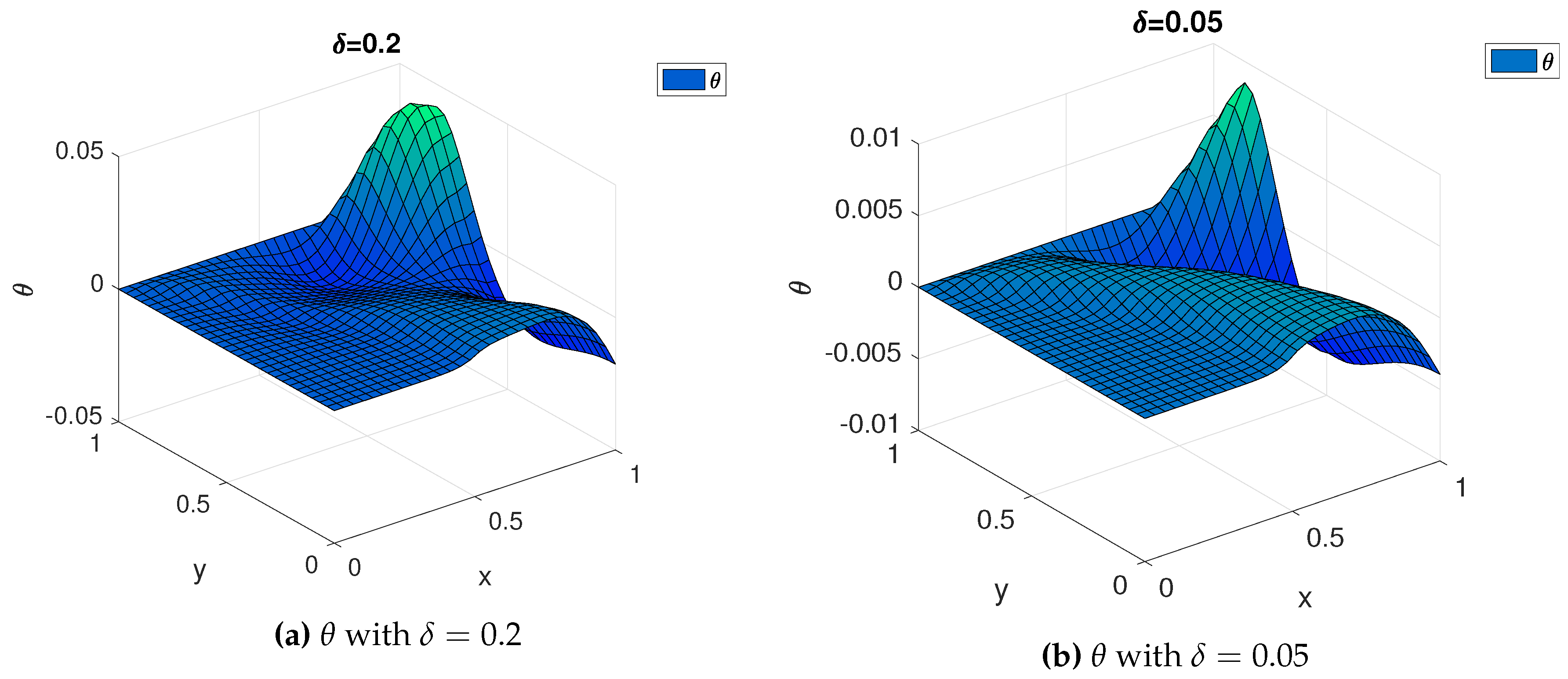
We solve the problem using the perturbation of Equation (30) and with the numerical scheme of Equation (21), getting two solutions, ${\rho }_p(x,y,t)$ and ${\rho }_u(x,y,t)$, where ${\rho }_p$ is the analytical solution using the perturbation and ${\rho }_u$ is the solution obtained with the numerical scheme. We plot the difference of $\theta ={\rho }_p-{\rho }_u$ for different values of $\delta$. In other words, we show that the perturbation is advantageous when the boundary data are small perturbations of the homogeneous case. Notice that, when $\delta =4/5$, the numerical solution is exactly the one plotted in Figure 3. In Figure 5 and Figure 6, the function $\theta$ (absolute error) is plotted for decreasing values of $\delta$. As one can notice, the error decreases for decreasing $\delta$, as expected.

The good agreement in the comparison suggests that the perturbation is not only useful as an approximation for small density variation around the constant value (homogeneous system), but it also provides some faith that the numerical method is reliable and can be used to infer the density distribution with general boundary data.

7. Concluding Remarks

We investigated the thin film flow of an inhomogeneous fluid in which its viscosity was a function of the density. The constitutive equation for the class of fluids considered can be derived by assuming that the stored energy that depends on the gradient of the density [9]. We considered a channel flow driven by a given pressure gradient, and we assumed that the aspect ratio between the width and the length of the channel was such that we can use the lubrication approximation. We then focused on the leading order problem. The mathematical problem reduced to a nonlinear first order PDE for the density, where the coefficients are integral operators. The problem was solved numerically and plots that describe the evolution of the density in the fluid domain were displayed.

References

- Truesdell, C.; Noll, W. The Non-Linear Field Theories of Mechanics; Springer: Berlin, Germany, 1965. [Google Scholar]
- Anand, M.; Rajagopal, K. A note on the flows of inhomogeneous fluids with shear-dependent viscosities. Arch. Mech. 2005, 57, 417–428. [Google Scholar]
- Rajagopal, K. Multiple Natural Configuration in Continuum Mechanics; Technical Report; University of Pittsburgh: Pittsburgh, PA, USA, 1995. [Google Scholar]
- Rajagopal, K.; Srinivasa, A. On the thermomechanics of shape memory wires. Zeitschrift fur angewandte Mathematik und Physik ZAMP 1999, 50, 459–496. [Google Scholar]
- Rajagopal, K.; Srinivasa, A. A thermodynamic frame work for rate type fluid models. J. Non-Newton. Fluid Mech. 2000, 88, 207–227. [Google Scholar] [CrossRef]
- Rajagopal, K.; Srinivasa, A. Modeling anisotropic fluids within the frame- work of bodies with multiple natural configurations. J. Non-Newt. Fluid Mech. 2001, 99, 109–124. [Google Scholar] [CrossRef]
- Rao, I.; Rajagopal, K. A study of strain-induced crystallization of polymers. Int. J. Solids Struct. 2001, 38, 1149–1167. [Google Scholar] [CrossRef]
- Rao, I.; Rajagopal, K. A thermodynamic framework for the study of crystallization in polymers. Zeitschrift fur angewandte Mathematik und Physik ZAMP 2002, 53, 365–406. [Google Scholar] [CrossRef]
- Málek, J.; Rajagopal, K. On the modeling of inhomogeneous incompressible fluid-like bodies. Mech. Mater. 2006, 38, 233–242. [Google Scholar] [CrossRef]
- Massoudi, M.; Vaidya, A. Unsteady flows of inhomogeneous incompressible fluids. Int. J. Non-Linear. Mech. 2011, 46, 738–741. [Google Scholar] [CrossRef]
Figure 1.
Sketch of the system.
Figure 2.
Stencil for the 2D and 3D problems.
Figure 3.
and in the case (B1).
Figure 4.
and in the case (B2).
Figure 5.
for decreasing .
Figure 6.
© 2019 by the authors. Licensee MDPI, Basel, Switzerland. This article is an open access article distributed under the terms and conditions of the Creative Commons Attribution (CC BY) license (http://creativecommons.org/licenses/by/4.0/).
Share and Cite
MDPI and ACS Style
Fusi, L.; Farina, A.; Rosso, F.; Rajagopal, K. Thin-Film Flow of an Inhomogeneous Fluid with Density-Dependent Viscosity. Fluids 2019, 4, 30. https://doi.org/10.3390/fluids4010030
AMA Style
Fusi L, Farina A, Rosso F, Rajagopal K. Thin-Film Flow of an Inhomogeneous Fluid with Density-Dependent Viscosity. Fluids. 2019; 4(1):30. https://doi.org/10.3390/fluids4010030
Chicago/Turabian StyleFusi, Lorenzo, Angiolo Farina, Fabio Rosso, and Kumbakonam Rajagopal. 2019. "Thin-Film Flow of an Inhomogeneous Fluid with Density-Dependent Viscosity" Fluids 4, no. 1: 30. https://doi.org/10.3390/fluids4010030