Article

Non-Iterative Partitioned Methods for Uncoupling Evolutionary Groundwater–Surface Water Flows

1
Department of Mathematics, Middlebury College, Middlebury, VT 05753, USA
2
Computer Science and Mathematics Division, Oak Ridge National Laboratory, Oak Ridge, TN 37831, USA
*
Author to whom correspondence should be addressed.
Fluids 2017, 2(3), 47; https://doi.org/10.3390/fluids2030047
Submission received: 1 July 2017 / Revised: 22 August 2017 / Accepted: 26 August 2017 / Published: 10 September 2017
(This article belongs to the Special Issue Turbulence: Numerical Analysis, Modelling and Simulation)

Abstract

:
We present an overview of a modern, efficient approach for uncoupling groundwater–surface water flows governed by the fully evolutionary Stokes–Darcy equations. Referred to as non-iterative partitioned methods, these algorithms treat the coupling terms explicitly and at each time level require only one Stokes and one Darcy sub-physics solve, thus taking advantage of existing solvers optimized for each sub-flow. This strategy often results in a time-step condition for stability. Furthermore, small problem parameters, specifically those related to the physical characteristics of the porous media domain, can render certain time-step conditions impractical. Despite these obstacles, researchers have made significant progress towards efficient, stable, and accurate partitioned methods. Herein, we provide a comprehensive survey and comparison of recent developments utilizing these non-iterative numerical schemes.

1. Introduction

Access to the clean freshwater is absolutely imperative for the continued survival of humankind. As a necessity for our agricultural, industrial and domestic practices, water constitutes an integral part of all civilizations. However, only 2.5% of the water present on Earth is freshwater, and the majority of this amount is either frozen or inaccessible. Furthermore, 96% of accessible freshwater comes from aquifers underground. Because of the scarcity of this resource, we must prioritize the protection and conservation of groundwater sources. Too often, human and natural processes threaten groundwater quality, sometimes irreversibly. For example, in hydro-fracturing, companies inject a mixture of water with sand and chemicals at high pressure into a well to create fractures to allow for the collection of shale gas. Companies do not recover the majority of the chemicals in this mixture and many fear that eventually these pollutants will leave the well to contaminate the local groundwater supply. Pesticide application in agriculture can have devastating effects on surrounding freshwater resources due to chemical run-off into nearby rivers, lakes, and streams, and seepage deep into the soil. Furthermore, many storage facilities for radioactive materials exist underground for both safety and convenience. Over time, as storage containers become compromised, nuclear waste can migrate into nearby freshwater aquifers. Even natural processes may result in contaminated freshwater, as evident in the devastation of forests growing above coastal aquifers from salt-water intrusion.
Tracking these contaminants necessitates accurate numerical models for this coupled flow. Scientists have thoroughly studied the individual groundwater and surface water flows (see, for example, Pinder and Celia [1], Watson and Burnett [2], or Bear [3] for an extensive study on subsurface flows, and Kundu, Cohan and Dowling [4] for surface water flows). As a result, many accurate and efficient solvers for the independent flow processes exist. Modeling the interaction of groundwater and surface water, however, presents additional difficulties as we must preserve the physical processes in each sub-flow while accurately describing the activity occurring along the interface.
An attractive and practical strategy, which is the main focus of this survey paper, is to make use of the existing solvers for separate fluid and porous media flow by investigating methods that uncouple the flow equations in time so that the individual flow problems may be solved separately. Called partitioned methods (also domain decomposition methods), these methods allow us to utilize, in a black-box manner, solvers already optimized for the separate flow problems. It is important that the partitioned methods maintain stability and accuracy along the interface where the two flows meet. In addition, potentially small physical parameters create an additional challenge for stability. We are concerned with methods that are efficient for the time-dependent models, in particular, the ones that are stable over long-time intervals, since groundwater moves slowly and numerical simulations may span long-time periods. Along these same lines, we want methods that converge within a reasonable amount of time to be of practical use, making higher-order convergence a desirable property.
In recent years, several researchers have made substantial progress in the development of non-iterative, partitioned methods applied to the evolutionary groundwater–surface water flow problem. Based on an implicit discretization in time for each subproblem, these methods, however, make use of results from previous time steps to predict the values on the interface at the current time step, thus requiring only one solve for groundwater and one solve for surface water flow at each time level (thus non-iterative). In this work, we will review and discuss several such methods so as to illustrate the current status of this important problem. The modeling of coupled fluid-porous media flow begins with the coupling of the Stokes or Navier–Stokes equations describing the flow in the fluid region, along with the Darcy or Brinkman equations for the flow in the aquifer, or porous media region containing the groundwater. This survey focuses on the Stokes–Darcy coupling that is suitable for slow moving flows over large domains.
Studies on the continuum surface water-groundwater model have been performed in [5,6,7,8]. The literature on numerical analysis of methods for the coupled Stokes–Darcy problem has grown extensively since [9,10] (see, for example, [11,12,13] for analysis of the steady-state problem). There exist many effective and efficient domain decomposition techniques for decoupling the Stokes–Darcy system in the stationary case [14,15,16,17,18,19,20,21,22,23,24]. To solve the fully evolutionary Stokes–Darcy problem, one approach is monolithic discretization by an implicit scheme (see, e.g., [25,26]). These schemes can also be solved by an iterative domain decomposition method at each time step. In general, any decoupling technique for stationary Stokes–Darcy (many cited above) may be applied to find the solution at each time level in the time-dependent case.
Non-iterative partitioned methods, an alternative approach, are advantageous in that they allow uncoupling into only one (SPD) Stokes and one (SPD) Darcy system per time step. Mu and Zhu presented the first non-iterative partitioned scheme in [27], proposing employing Backward Euler discretization for each subproblem while treating the coupling term explicitly by Forward Euler. Layton, Tran and Trenchea revisited this method in [28], with an improved analysis showing long-time stability. In that work, the authors also developed and tested for efficiency a second first-order scheme, Backward Euler–Leap Frog. Following these methods, others proposed several other implicit-explicit (IMEX) methods of high order, such as Crank–Nicolson–Leap Frog [29], second-order backward-differentiation with Gear’s extrapolation [30], and Adam–Moulton–Bashforth [30,31]. Although these methods use explicit discretizations for the coupling terms, all are now known to be long-time stable and optimally convergent uniformly in time (possibly under a small time-step constraint). With the addition of suitable stabilization terms, it is possible to further enhance the stability property, for instance, a stabilized Crank–Nicolson–Leap Frog, developed in [32,33], requires no time-step restriction for the long-time stability and convergence. Another way for uncoupling groundwater–surface water systems is using splitting schemes. Unlike the aforementioned IMEX schemes that solve for separate sub-flows in parallel, splitting methods require sequential sub-problem solves at each time step. In [34], the authors proposed four first and second-order splitting schemes. Theoretical and numerical evidence provided therein suggests that these methods are stable for larger time steps than the first order IMEX schemes and, in particular, a good option in case of small physical parameters. Finally, asynchronous (aka, multiple-time-step, multi-rate) partitioned methods allow for different time steps in the two subregions, motivated by the observation that the flow in fluid region occurs with higher velocities compared to flow in porous media region. Such methods may be more efficient, as we may apply two different time steps to separately solve the fast and slow flows. Developed in [35,36], these asynchronous techniques utilize the Backward Euler-Forward Euler time discretization, with long-time stability acquired in the latter work.
We organize this paper as follows. Section 2 reviews the preliminaries of the Stokes–Darcy equation, including interface conditions, variational formulation and semi-discrete approximations. We briefly discuss the implicit time discretization, together with the iterative domain-decomposition approach. Section 3 focuses on first-order partitioned methods. We will survey several different approaches including first-order IMEX schemes and splitting schemes. We review high-order methods in Section 4 and asynchronous partitioned techniques in Section 5. Finally, we provide some conclusions and outlooks in Section 6.

2. The Stokes–Darcy Equation

Let the fluid region be denoted by Ω f and the porous media region by Ω p . Assume both domains are bounded and regular. Let I represent the interface between the two domains. We assume the time-dependent Stokes flow in Ω f and the time-dependent groundwater flow along with Darcy’s law in Ω p . The Stokes–Darcy equation, describing the fluid velocity field u = u ( x , t ) and pressure p = p ( x , t ) on Ω f and the porous media hydraulic head ϕ = ϕ ( x , t ) on Ω p , can be written as follows:
u t ν Δ u + p = f f , · u = 0 , in Ω f , S 0 ϕ t · K ϕ = f p , in Ω p , u ( x , 0 ) = u 0 , in Ω f and ϕ ( x , 0 ) = ϕ 0 , in Ω p , u ( x , t ) = 0 , in Ω f \ I and ϕ ( x , t ) = 0 , in Ω p \ I , + coupling conditions across I .
Here, f f denotes the body force in the fluid region, f p is the sink or source in the porous media region, ν > 0 is the kinematic viscosity of the fluid, S 0 is the specific mass storativity coefficient and K is the hydraulic conductivity tensor, assumed to be symmetric, positive definite with spectrum ( K ) [ k min , k max ] .
It is worth noting that values of S 0 and the smallest eigenvector k min of K can be very small (see Table 1 and Table 2 for the values of S 0 and k min for different materials). As we shall see, this poses a major challenge in designing partitioned methods with good stability. Indeed, partitioning often induces time-step restrictions for long-time stability, which may become severe in the case of small system parameters.

2.1. Interface Conditions

To close the coupled problem formulation, a set of conditions has to be defined on the interface. Let n ^ f / p denote the indicated, outward pointing, unit normal vector on I. The first two coupling conditions involve the conservation of mass and balance of forces on I:
u · n ^ f K ϕ · n ^ p = 0 , on I , p ν n ^ f · u · n ^ f = g ϕ on I .
In addition, we need a tangential condition on the fluid region’s velocity along the interface. In [5], Beavers and Joseph proposed the following slip–flow condition, expressing that slip velocity along I is proportional to the shear stresses along I
ν τ ^ i · u · n ^ f = α B J ν g τ ^ i · K · τ ^ i ( u u p ) · τ ^ i , on I for any τ ^ i tangent vector on I ,
where α B J is a dimensionless constant depending solely on the porous media properties and ranges from 0.01 to 5, g is the gravitational acceleration constant, and u p is the average velocity in the porous media region. The validity of Beavers–Joseph interface condition has been supported by abundant empirical evidence; however, one challenge in adopting this condition is that the bilinear form in the weak formulation is not coercive. Several simplifications have been considered. In [6], Saffman proposed a modification to the Beavers–Joseph coupling condition by dropping the porous media averaged velocity u p , based on observations that the term u p · τ ^ i is negligible compared to the fluid velocity u · τ ^ i . This simplified condition was mathematically justified in [39] and has been shown satisfactory for many fluid-porous media systems. Known as Beavers–Joseph–Saffman(–Jones) coupling condition, this is the third and final condition we use in this article:
ν τ ^ i · u · n ^ f = α B J ν g τ ^ i · K · τ ^ i u · τ ^ i , on I for any τ ^ i tangent vector on I .
For the analysis and numerical methods for Stokes–Darcy systems with Beavers–Joseph condition, we refer to [21,26,40].

2.2. Variational Formulation and Semi-Discrete Approximations Using Finite Element Method

We denote the L 2 ( I ) norm by · I and the L 2 ( Ω f / p ) norms by · f / p , respectively, and the corresponding inner products are denoted by ( · , · ) f / p . In addition, define the H div ( Ω f ) and H 1 ( Ω f / p ) norms
u div , f : = u f 2 + · u f 2 , u 1 , f / p = u f / p 2 + u f / p 2 ,
the functional spaces
X f = { v H 1 ( Ω f ) d : v = 0 on Ω f \ I } , Q f = L 2 ( Ω f ) , X p = { ψ H 1 ( Ω p ) : ψ = 0 on Ω p \ I } ,
and the bilinear forms
a f ( u , v ) = ( ν u , v ) f + i I α B J ν g τ ^ i · K · τ ^ i ( u · τ ^ i ) ( v · τ ^ i ) d s , a p ( ϕ , ψ ) = g ( K ϕ , ψ ) p , and c I ( u , ϕ ) = g I ϕ u · n ^ f d s .
It can be shown that a f / p ( · , · ) are continuous and coercive.
A (monolithic) variational formulation of the coupled problem is to find ( u , p , ϕ ) : [ 0 , ) X f × Q f × X p satisfying the given initial conditions and, for all v X f , q Q f , ψ X p ,
( u t , v ) f + a f ( u , v ) ( p , · v ) f + c I ( v , ϕ ) = ( f f , v ) f , ( q , · u ) f = 0 , g S 0 ( ϕ t , ψ ) p + a p ( ϕ , ψ ) c I ( u , ψ ) = g ( f p , ψ ) p .
Note that, setting v = u , ψ = ϕ and adding, the coupling terms exactly cancel out in the monolithic sum yielding the energy estimate for the coupled system.
To discretize the Stokes–Darcy problem in space by the finite element method (FEM), we select finite element spaces
velocity : X f h X f , Darcy pressure : X p h X p , Stokes pressure : Q f h Q f
based on a conforming FEM triangulation with maximum triangle diameter denoted by “h”. We do not assume mesh compatibility or interdomain continuity at the interface I between the FEM meshes in the two subdomains. The Stokes velocity-pressure FEM spaces are assumed to satisfy the usual discrete inf-sup condition for stability of the discrete pressure (see, e.g., [41])
β h > 0 such that inf q h Q f h , q h 0 sup v h X f h , v h 0 ( q h , · v h ) f v h f q h f > β h .
Assume X f h , X p h , Q f h satisfy approximation properties of piecewise polynomials on quasi-uniform meshes of local degrees k , k , k 1 , respectively, that is,
inf v h X f h u v h f C h k + 1 u H k + 1 ( Ω f ) , u H k + 1 ( Ω f ) , inf v h X f h ( u v h ) f C h k u H k + 1 ( Ω f ) , u H k + 1 ( Ω f ) , inf ψ h X p h ϕ ψ h p C h k + 1 ϕ H k + 1 ( Ω p ) , ϕ H k + 1 ( Ω p ) , inf ψ h X p h ( ϕ ψ h ) p C h k ϕ H k + 1 ( Ω p ) , ϕ H k + 1 ( Ω p ) , inf q h Q f h p q h f C h k p H k ( Ω f ) , p H k ( Ω f ) .
The semi-discretization for the time-dependent Stokes–Darcy problem is as follows: find ( u h , p h , ϕ h ) : [ 0 , ) X f h × Q f h × X p h satisfying the given initial conditions and, for all v h X f h , q h Q f h , ψ h X p h ,
( u h , t , v h ) f + a f ( u h , v h ) ( p h , · v h ) f + c I ( v h , ϕ h ) = ( f f , v h ) f , ( q h , · u h ) f = 0 , g S 0 ( ϕ h , t , ψ h ) p + a p ( ϕ h , ψ h ) c I ( u h , ψ h ) = g ( f p , ψ h ) p .
It is worth noting that the coupling between the Stokes and the Darcy sub-problems is exactly skew symmetric.

2.3. Fully-Discrete Approximations with Fully Implicit Temporal Schemes

Let t n : = n Δ t and w n : = w ( x , t n ) for any function w ( x , t ) . For V being a Banach space with norm · V , we denote the following discrete norms
| w | L 2 ( 0 , T ; V ) : = Δ t n = 0 N w n V 2 1 / 2 , | w | L ( 0 , T ; V ) : = sup 0 n N w n V ,
where N = T / Δ t and T can be . For fixed T > 0 , the discrete norm | · | L ( 0 , T ; V ) is bounded by the continuous norm · L ( 0 , T ; V ) . The discrete norm | · | L 2 ( 0 , T ; V ) , on the other hand, depends on the time step Δ t . However, for functions smooth in time, this norm converges to the continuous norm · L 2 ( 0 , T ; V ) as Δ t 0 . In those cases, one can reasonably assume the uniform bound of | · | L 2 ( 0 , T ; V ) , independent of Δ t .
The most natural time discretization for the Stokes–Darcy equation is perhaps the first-order backward Euler scheme, which, in combination with the aforementioned finite element Galerkin method for the spatial discretization, leads to the following fully implicit, coupled problem.
Algorithm 1  Backward Euler
Given ( u h n , p h n , ϕ h n ) X f h × Q f h × X p h , find ( u h n + 1 , p h n + 1 , ϕ h n + 1 ) X f h × Q f h × X p h such that for all v h X f h , q h Q f h , ψ h X p h ,
( u h n + 1 u h n Δ t , v h ) f + a f ( u h n + 1 , v h ) ( p h n + 1 , · v h ) f + c I ( v h , ϕ h n + 1 ) = ( f f n + 1 , v h ) f , ( q h , · u h n + 1 ) f = 0 , g S 0 ( ϕ h n + 1 ϕ h n Δ t , ψ h ) p + a p ( ϕ h n + 1 , ψ h ) c I ( u h n + 1 , ψ h ) = g ( f p n + 1 , ψ h ) p .
Stability and convergence analysis of this scheme were conducted in [25,26,27], for both Beavers–Joseph and Beavers–Joseph-Saffman–Jones interface conditions. Higher order fully implicit schemes, such as the Crank–Nicolson, can also be considered. In general, fully implicit methods possess superior stability compared to IMEX or splitting temporal schemes. The major concern here is that this approach must solve a coupled problem at each time level. Partitioning the coupled problem at each time step is possible, but involves an iterative procedure with additional cost. In principle, any decoupled methods developed for the stationary model can be used in iteration at each time level.

3. First Order Partitioned Schemes

An attractive alternative to fully implicit, fully coupled discretization is exploiting information obtained in previous time steps to construct a non-iterative uncoupling scheme, which only need a single Stokes solve and a single Darcy solve at each time step. This approach allows the use of legacy subproblems’ codes and obviously requires less programming effort (compared to solving coupled Stokes–Darcy system directly) as well as less computation cost (compared to iterative domain decomposition approach). As the interface values are obtained in an explicit manner, the main challenge here is how to obtain optimal accuracy and good stability properties. Many non-iterative partitioned methods have been developed in the literature recently [27,28,29,30,31,32,33,34,35,36,42], whose stability and accuracy have been proved (over a long time or without time-step condition) and numerically tested. Several of them maintain good performance even in the case of small parameters. The rest of this paper represents an overview of these developments. Our discussion will be divided into three parts: in Section 3, we survey first order schemes; in Section 4, high order schemes will be discussed; Section 5 is devoted to asynchronous partitioned methods. Unless otherwise stated, C denotes a generic positive constant whose value may be different from place to place but which is independent of mesh size, time step, and final time. For all the methods surveyed, approximations are needed at the first few (one or more) time steps to begin, and we always assume these are computed to sufficient accuracy.

3.1. Backward Euler-Forward Euler

The first non-iterative uncoupling scheme is Backward Euler-Forward Euler (BEFE), proposed by Mu and Zhu in [27] (and referred to as DBES therein). This method applies Backward Euler discretization for the subproblems and treats the coupling terms by explicit Forward Euler:
Algorithm 2  Backward Euler-Forward Euler (BEFE)
Given ( u h n , p h n , ϕ h n ) X f h × Q f h × X p h , find ( u h n + 1 , p h n + 1 , ϕ h n + 1 ) X f h × Q f h × X p h such that for all v h X f h , q h Q f h , ψ h X p h ,
( u h n + 1 u h n Δ t , v h ) f + a f ( u h n + 1 , v h ) ( p h n + 1 , · v h ) f + c I ( v h , ϕ h n ) = ( f f n + 1 , v h ) f , ( q h , · u h n + 1 ) f = 0 , g S 0 ( ϕ h n + 1 ϕ h n Δ t , ψ h ) p + a p ( ϕ h n + 1 , ψ h ) c I ( u h n , ψ h ) = g ( f p n + 1 , ψ h ) p .
A stability analysis for BEFE was given in [27]. These results only apply for bounded time intervals [ 0 , T ] with T < , as the estimates include e c T multipliers and thus grow exponentially with T. The long-time stability of BEFE was established in [28]. An important feature of this proof, also of other long-time results coming next, is that no form of Gronwall’s inequality was used. This result can be stated as follows.
Proposition 1
(Long-time stability of BEFE, [28]). Consider the scheme BEFE. Assume the following time-step condition is satisfied
Δ t min { ν k min 2 , S 0 ν 2 k min } .
Then, the following hold:
(i) 
If f f L ( 0 , ; L 2 ( Ω f ) ) , f p L ( 0 , ; L 2 ( Ω p ) ) , then
u h n f 2 + ϕ h n p 2 C , n 0 .
(ii) 
If | f f | L 2 ( 0 , ; L 2 ( Ω f ) ) and | f p | L 2 ( 0 , ; L 2 ( Ω p ) ) are uniformly bounded in Δ t , then
u h n f 2 + ϕ h n p 2 + Δ t = 0 n u h f 2 + ϕ h p 2 C , n 0 .
BEFE is first order in time. A convergence analysis of this scheme can be found in [27], with a very recent improvement in [43].

3.2. Backward Euler–Leap Frog

Backward Euler–Leap Frog (BELF) is another IMEX scheme, first proposed in [28]. This method is a combination of the three level implicit method with the coupling terms treated by the explicit Leap-Frog method. Approximations are needed at the first two time steps to begin. The stability region of the usual Leap-Frog time discretization for y = λ y is exactly the interval of the imaginary axis 1 Im ( Δ t λ ) + 1 . Thus, LF is unstable for every problem except for ones that are exactly skew symmetric such as the coupling herein.
The Backward Euler–Leap Frog scheme can be formulated as follows:
Algorithm 3  Backward Euler–Leap Frog (BELF)
Given ( u h n 1 , p h n 1 , ϕ h n 1 ) , ( u h n , p h n , ϕ h n ) X f h × Q f h × X p h , find ( u h n + 1 , p h n + 1 , ϕ h n + 1 ) X f h × Q f h × X p h such that for all v h X f h , q h Q f h , ψ h X p h ,
( u h n + 1 u h n 1 2 Δ t , v h ) f + a f ( u h n + 1 , v h ) ( p h n + 1 , · v h ) f + c I ( v h , ϕ h n ) = ( f f n + 1 , v h ) f , ( q h , · u h n + 1 ) f = 0 , g S 0 ( ϕ h n + 1 ϕ h n 1 2 Δ t , ψ h ) p + a p ( ϕ h n + 1 , ψ h ) c I ( u h n , ψ h ) = g ( f p n + 1 , ψ h ) p .
As with any explicit scheme, BELF inherits a time-step restriction for the stability. The following long-time stability result was established in [28].
Proposition 2
(Long-time stability of BELF, [28]). Consider the scheme BELF. Assume that the following time-step condition is satisfied
Δ t min { ν k min , S 0 ν k min , ν k min 2 , S 0 ν 2 k min } ;
then, BELF possesses the same stability properties as those for BEFE in Proposition 1. More precisely,
(i) 
If f f L ( 0 , ; L 2 ( Ω f ) ) , f p L ( 0 , ; L 2 ( Ω p ) ) , then
u h n f 2 + ϕ h n p 2 C , n 0 .
(ii) 
If | f f | L 2 ( 0 , ; L 2 ( Ω f ) ) , | f p | L 2 ( 0 , ; L 2 ( Ω p ) ) are uniformly bounded in Δ t , then
u h n f 2 + ϕ h n p 2 + Δ t = 0 n u h f 2 + ϕ h p 2 C , n 0 .
It was also proved that BELF achieves the optimal convergence rate uniformly in time, as shown below.
Proposition 3
(Error estimate of BELF, [28])
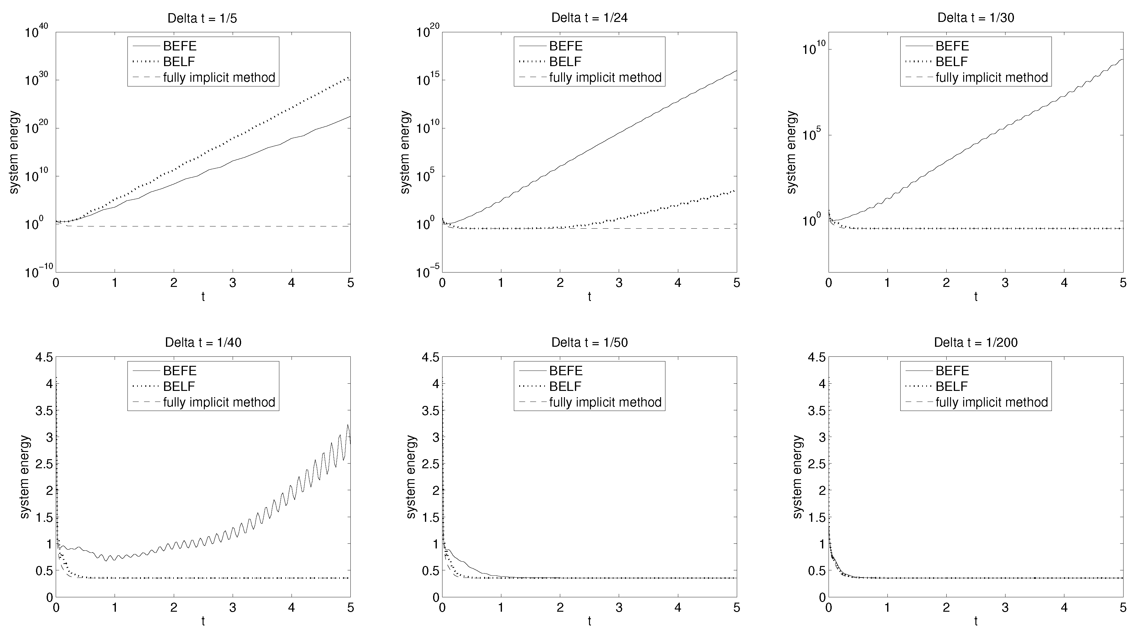
. Consider the scheme BELF. Assume the following time-step condition is satisfied
Δ t min { ν k min , S 0 ν k min , ν k min 2 , S 0 ν 2 k min } ,
as in Proposition 2. If the solution of the Stokes–Darcy problem (1) is long-time regular in the sense that
u W 2 , ( 0 , ; L 2 ( Ω f ) ) W 1 , ( 0 , ; H k + 1 ( Ω f ) ) , ϕ W 2 , ( 0 , ; L 2 ( Ω p ) ) W 1 , ( 0 , ; H k + 1 ( Ω p ) ) , p L ( 0 , ; H k ( Ω f ) ) ,
then the solution of BELF satisfies the uniform in time error estimates
u ( t n ) u h n f 2 + ϕ ( t n ) ϕ h n p 2 C ( Δ t 2 + h 2 k ) , n 0 .
Numerical tests illustrating the theoretical stability and convergence properties of BEFE and BELF were presented in [28]. In particular, the stability of these two methods is compared to that of the fully implicit method in the case of small k min for a Stokes–Darcy flow on Ω f = ( 0 , 1 ) × ( 1 , 2 ) and Ω p = ( 0 , 1 ) × ( 0 , 1 ) with the interface I = ( 0 , 1 ) × { 1 } . Given the source terms f f 0 , f p 0 , the initial condition
u ( x , y , 0 ) = x 2 ( y 1 ) 2 + y , 2 3 x ( y 1 ) 3 + 2 π sin ( π x ) , p ( x , y , 0 ) = ( 2 π sin ( π x ) ) sin π 2 y , ϕ ( x , y , 0 ) = ( 2 π sin ( π x ) ) ( 1 y cos ( π y ) ) ,
set all the physical parameters (except for ν and k min ) to 1. Letting h = 1 10 , ν = 1 10 , the evolution of the energy E n = u h n f 2 + ϕ h n p 2 with k min = 10 6 is shown in Figure 1. Since the true solution decays as t , any growth in E n indicates instability. The plot reveals that while not unconditionally stable like the fully implicit method, BEFE and BELF only require mild constraints on Δ t for their stability. Indeed, BELF is already stable for Δ t 1 30 , followed by BEFE at Δ t 1 50 . These conditions are much weaker than those predicted by the theory.
In summary, the first-order IMEX methods BEFE and BELF allow a parallel, non-iterative uncoupling of the Stokes–Darcy system at each time step and, on the other hand, enjoy the desirable strong stability and convergence properties. One disadvantage, as shown in their time-step restrictions, is that they may become highly unstable when one of the parameters S 0 and k min is small. In the next subsection, this constraint is relaxed with another type of first-order partitioned methods, splitting schemes.

3.3. First Order Sequential Splitting Schemes

In [34], several methods for non-iterative, sub-physics uncoupling the evolutionary Stokes–Darcy problem were proposed, using ideas from splitting methods. The estimates and tests therein suggest that these methods are stable for larger timesteps than the IMEX based partitioned methods BEFE and BELF, and in particular, a very good option when either k min or S 0 (but not both) is small. Here, the Stokes and Darcy systems are uncoupled, but, unlike the aforementioned IMEX schemes, sequentially solved.
In the first Backward Euler time-split (BEsplit1) scheme, the coupling term in the ϕ equation is evaluated at the newly computed value u h n + 1 so we compute ϕ h n u h n + 1 ϕ h n + 1 .
Algorithm 4  Backward Euler time-split 1 (BEsplit1)
Given ( u h n , p h n , ϕ h n ) X f h × Q f h × X p h , find ( u h n + 1 , p h n + 1 , ϕ h n + 1 ) X f h × Q f h × X p h such that for all v h X f h , q h Q f h , ψ h X p h ,
( u h n + 1 u h n t , v h ) f + a f ( u h n + 1 , v h ) ( p h n + 1 , · v h ) f + c I ( v h , ϕ h n ) = ( f f n + 1 , v h ) f , ( q h , · u h n + 1 ) f = 0 , g S 0 ( ϕ h n + 1 ϕ h n t , ψ h ) p + a p ( ϕ h n + 1 , ψ h ) c I ( u h n + 1 , ψ h ) = g ( f p n + 1 , ψ h ) p .
The long-time stability of this scheme can be stated as follows.
Proposition 4
(Long-time stability of BEsplit1, [34]). Consider the scheme BEsplit1. Assume the following time-step condition is satisfied:
Δ t max { S 0 ν k min , S 0 h , S 0 ν h , k min } .
If | f f | L 2 ( 0 , ; L 2 ( Ω f ) ) and | f p | L 2 ( 0 , ; L 2 ( Ω p ) ) are uniformly bounded in Δ t , then
u h n f 2 + ϕ h n p 2 C , n 0 .
The second Backward Euler time-split (BEsplit2) is the previous method in the opposite order, i.e., computing u h n ϕ h n + 1 u h n + 1 . The analysis in [34] revealed that control was needed for a term u h n + 1 u h n div . This led to the insertion of the grad-div stabilization term ( · ( u h n + 1 u h n ) / Δ t , · v h ) acting on the time discretization of u t . This term is exactly zero for the continuous problem so it does not increase the method’s consistency error.
Algorithm 5  Backward Euler time-split 2 (BEsplit2)
Given ( u h n , p h n , ϕ h n ) X f h × Q f h × X p h , find ( u h n + 1 , p h n + 1 , ϕ h n + 1 ) X f h × Q f h × X p h such that for all v h X f h , q h Q f h , ψ h X p h ,
g S 0 ( ϕ h n + 1 ϕ h n Δ t , ψ h ) p + a p ( ϕ h n + 1 , ψ h ) c I ( u h n , ψ h ) = g ( f p n + 1 , ψ h ) p , ( u h n + 1 u h n Δ t , v h ) f + · u h n + 1 u h n Δ t , · v h f + a f ( u h n + 1 , v h ) ( p h n + 1 , · v h ) f + c I ( v h , ϕ h n + 1 ) = ( f f n + 1 , v h ) f , ( q h , · u h n + 1 ) f = 0 .
The stability result of BEsplit2 is presented below.
Proposition 5
(Long-time stability of BEsplit2, [34]). Consider the scheme BEsplit2. Assume the following time-step condition is satisfied
Δ t max { S 0 ν k min , S 0 h , k min h , k min } .
If | f f | L 2 ( 0 , ; L 2 ( Ω f ) ) and | f p | L 2 ( 0 , ; L 2 ( Ω p ) ) are uniformly bounded in Δ t , then
u h n f 2 + ϕ h n p 2 + Δ t = 0 n u h f 2 + ϕ h p 2 C , n 0 .
Propositions 4 and 5 impose two slightly different conditions on Δ t , both of which are mild when one of S 0 and k min is small. In those cases, BEsplit1 and BEsplit2 are preferable choices to first-order IMEX schemes, with the small price of solving the uncoupled subproblems sequentially, instead of in parallel. However, it is worth remarking that these methods may become unstable if both parameters are small. Finally, BEsplit1 and BEsplit2 can be shown to be optimally convergent under the same time-step conditions for stability. For a thorough analysis, we refer to [44].
Two other splitting methods were proposed in [34], whose details are omitted here for brevity. SDsplit is a first order scheme, long-time stable under the condition Δ t min S 0 , k m i n h , and thus seems less favorable than BEsplit1 and BEsplit2 in theory. CNsplit, on the other hand, is stable with Δ t S 0 h and a very good option in case of small k min . This scheme is second order.
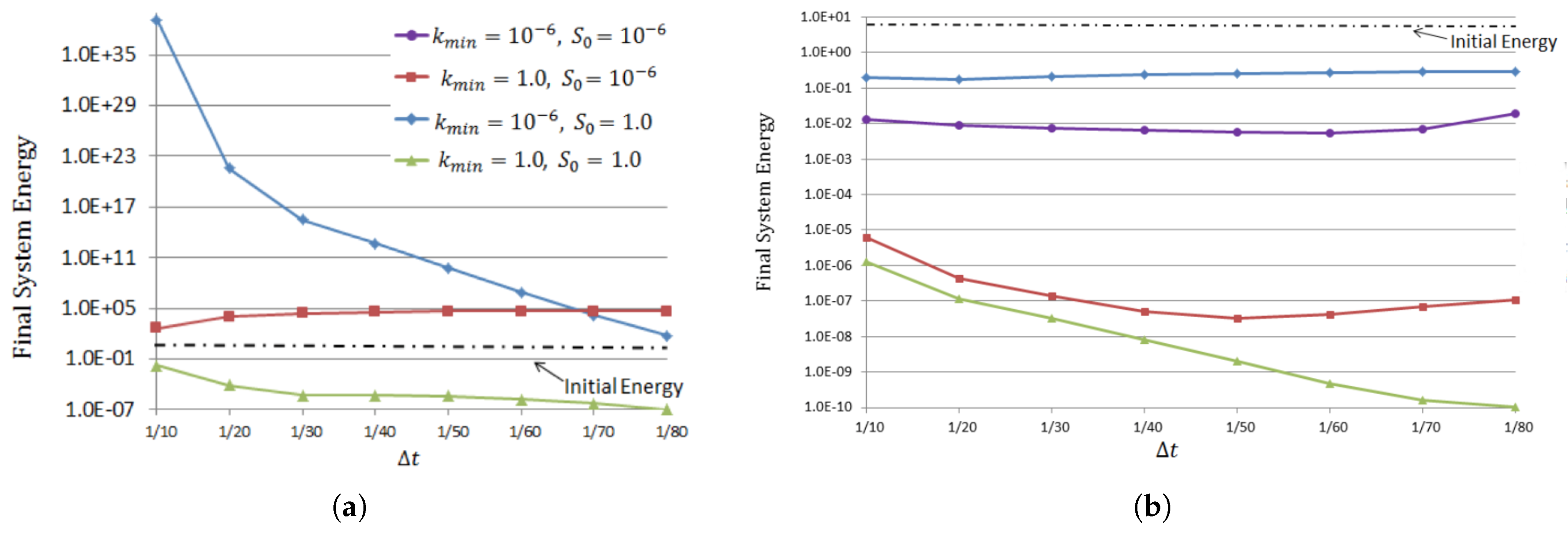
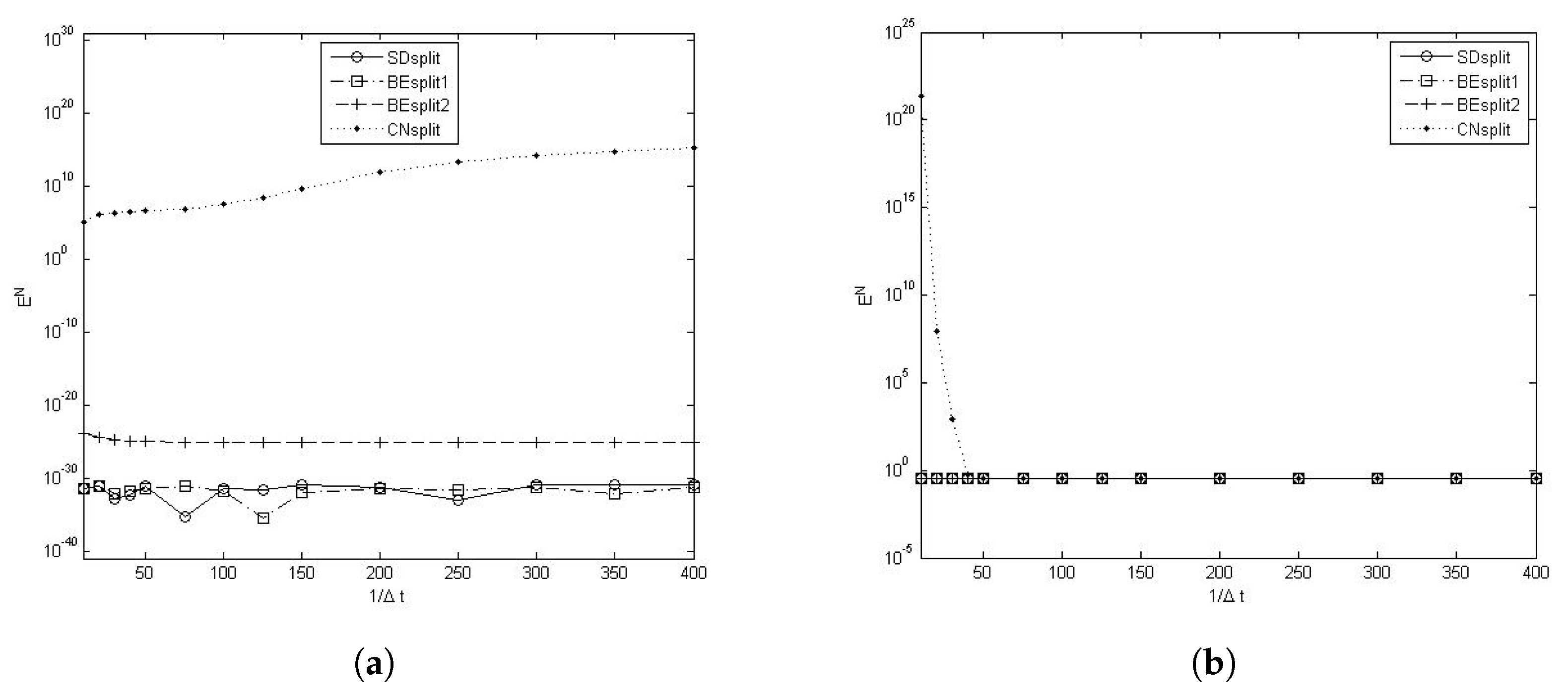
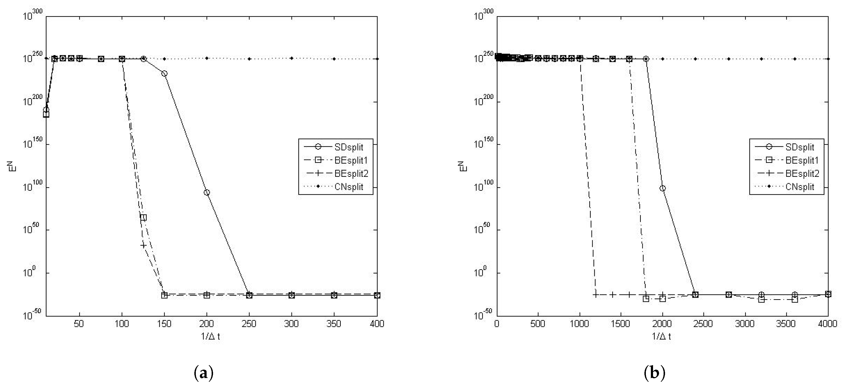
Numerical tests checking and comparing the largest time step for which the four methods are stable over long-time intervals were also performed in [34]. Taking the initial condition as in (3), the body sources to be 0, the system parameters (except k min and S 0 ) to be 1.0 and mesh size h = 1 10 , the authors computed the system energy E N at final time T = 10 with different time-step sizes. Since the true solution decays as t , large E N indicates instability. The performance of presented splitting methods was plotted for three cases: (i) O ( 1 ) k min and small S 0 , (ii) small k min and O ( 1 ) S 0 , and (iii) small k min and small S 0 (see Figure 2 and Figure 3). These plots show that for small parameter k min or S 0 , BEsplit1 and BEsplit2 are stable for large time steps. The performance of SDsplit is close to those of BEsplit1 and BEsplit2, suggesting that its theoretical condition was not optimized. These three first order splitting methods display superior stability to IMEX methods in our previous tests. The second order CNsplit in general requires a much smaller time step, but still possesses strong stability in the case of small k min and large S 0 .

4. High Order Partitioned Schemes

In this section, we review recent developments in high-order partitioned schemes for uncoupling the Stokes–Darcy system. Thus far, most of the proposed methods are of IMEX type (except for CNsplit, which was mentioned above). The IMEX schemes we will discuss in detail here include Crank–Nicolson–Leap Frog [29,32,33], second-order backward-differentiation with Gear’s extrapolation [30], and Adam-Moulton-Bashforth [30,31].

4.1. Crank–Nicolson–Leap Frog

The Crank–Nicolson–Leap Frog (CNLF) method is a second-order scheme that employs the implicit Crank–Nicolson discretization of subdomain terms and treats the interface terms explicitly with Leap Frog. CNLF was developed for uncoupling systems of evolutionary equations in [45,46,47]. This method was first applied to uncouple Stokes–Darcy system in [29].
CNLF is a three-level method. The first terms, ( u h 0 , p h 0 , ϕ h 0 ) , arise from the initial conditions of the problem. To obtain ( u h 1 , p h 1 , ϕ h 1 ) , one must use another numerical method. Note that approximations in this first step will affect the overall convergence rate of the method, and as usual, we assume them to be sufficiently accurate. This scheme can be stated as follows:
Algorithm 6  Crank–Nicolson–Leap Frog (CNLF)
Given ( u h n 1 , p h n 1 , ϕ h n 1 ) , ( u h n , p h n , ϕ h n ) X f h × Q f h × X p h , find ( u h n + 1 , p h n + 1 , ϕ h n + 1 ) X f h × Q f h × X p h such that for all v h X f h , q h Q f h , ψ h X p h ,
u h n + 1 u h n 1 2 Δ t , v h f + a f u h n + 1 + u h n 1 2 , v h p h n + 1 + p h k 1 2 , · v h f + c I ( v h , ϕ h n ) = ( f f n , v h ) f , q h , · u h n + 1 + u h n 1 2 f = 0 , g S 0 ϕ h n + 1 ϕ h n 1 2 Δ t , ψ h p + a p ϕ h n + 1 + ϕ h n 1 2 , ψ h c I ( u h n , ψ h ) = g ( f p n , ψ h ) p .
CNLF provably possesses a strong stability and convergence properties, as shown in [29] and presented below. Specifically, the time-step condition for CNLF does not depend on k min , making this method a very good choice for fluid-porous media systems with small k min .
Proposition 6
(Long-time stability of CNLF, [29]). Consider the scheme CNLF. Assume the following time-step condition is satisfied:
Δ t max { min { h 2 , S 0 } , min { h , S 0 h } } .
If | f f | L 2 ( 0 , ; L 2 ( Ω f ) ) and | f p | L 2 ( 0 , ; L 2 ( Ω p ) ) are uniformly bounded in Δ t , then
u h n f 2 + ϕ h n p 2 C , n 0 .
Proposition 7
(Error estimate of CNLF, [29]). Consider the scheme CNLF. Assume the following time-step condition is satisfied:
Δ t max { min { h 2 , S 0 } , min { h , S 0 h } } ,
as in Proposition 6. If the solution of the Stokes–Darcy problem (1) is regular in the sense that
u H 1 ( 0 , ; H k + 1 ( Ω f ) ) L ( 0 , ; H k + 1 ( Ω f ) ) H 3 ( 0 , ; H 1 ( Ω f ) ) , ϕ H 1 ( 0 , ; H k + 1 ( Ω p ) ) L ( 0 , ; H k + 1 ( Ω p ) ) H 3 ( 0 , ; H 1 ( Ω p ) ) , p L 2 ( 0 , ; H k ( Ω f ) ) ,
and the discrete norms of u, p and ϕ in L 2 ( 0 , ; H k + 1 ( Ω f ) ) , L 2 ( 0 , ; H s + 1 ( Ω f ) ) , and L 2 ( 0 , ; H k + 1 ( Ω p ) ) are uniformly bounded in Δ t , then
u ( t n ) u h n f 2 + ϕ ( t n ) ϕ h n p 2 C ( Δ t 4 + h 2 k ) , n 0 .
While independent of k min , the conditional stability of CNLF may still be restrictive when faced with small S 0 . To tackle this difficulty, the authors of [32,33] proposed a strategy to improve the stability property of CNLF by adding appropriate stabilization terms to both the Stokes as well as the groundwater flow equation.
Algorithm 7  Stabilized Crank–Nicolson–Leap Frog (CNLFstab)
Given ( u h n 1 , p h n 1 , ϕ h n 1 ) , ( u h n , p h n , ϕ h n ) X f h × Q f h × X p h , find ( u h n + 1 , p h n + 1 , ϕ h n + 1 ) X f h × Q f h × X p h such that for all v h X f h , q h Q f h , ψ h X p h ,
u h n + 1 u h n 1 2 Δ t , v h f + · u h n + 1 u h n 1 2 Δ t , · v h f + a f u h n + 1 + u h n 1 2 , v h p h n + 1 + p h k 1 2 , · v h f + c I ( v h , ϕ h n ) = ( f f n , v h ) f , q h , · u h n + 1 f = 0 , g S 0 ϕ h n + 1 ϕ h n 1 2 Δ t , ψ h p + a p ϕ h n + 1 + ϕ h n 1 2 , ψ h c I ( u h n , ψ h ) + Δ t g 2 C f , p 2 ( ϕ h k + 1 ϕ h k 1 , ψ h ) p + ( ( ϕ h k + 1 ϕ h k 1 ) , ψ h ) p = g ( f p n , ψ h ) p .
The resulting numerical scheme, denoted CNLFstab, is unconditionally, uniformly in time stable, as well as second-order convergent. More specifically, it was shown in [33] that the added stabilization terms,
· u h n + 1 u h n 1 2 Δ t , · v h f , and Δ t g 2 C f , p 2 ( ϕ h k + 1 ϕ h k 1 , ψ h ) p + ( ( ϕ h k + 1 ϕ h k 1 ) , ψ h ) p ,
eliminate the time-step restriction without affecting the second-order accuracy of the method. Indeed, among all the methods we have discussed so far, CNLFstab exhibits the best stability and convergence properties. Here, C f , p is a constant satisfying
| c I ( u , ϕ ) | g C f , p u div , f ϕ 1 , p .
In the special case of a flat interface I, with Ω f and Ω p being arbitrary domains, C f , p equals 1 (see [48], Lemmas 3.1 and 3.2]).
We make the above discussion rigorous with the following results.
Proposition 8
(Long-time, unconditional stability of CNLFstab, [33]). Consider the scheme CNLFstab. If | f f | L 2 ( 0 , ; L 2 ( Ω f ) ) and | f p | L 2 ( 0 , ; L 2 ( Ω p ) ) are uniformly bounded in Δ t , then
u h n div , f 2 + ϕ h n p 2 C , n 0 .
Proposition 9
(Error estimate of CNLFstab, [33]). Consider the scheme CNLFstab. Assume u, p and ϕ satisfy the same regularity condition as in Proposition 7, then the solution of CNLFstab satisfies the unconditional, uniform in time error estimate
u ( t n ) u h n div , f 2 + ϕ ( t n ) ϕ h n p 2 C ( Δ t 4 + h 2 k ) , n 0 .
The stability and convergence properties of CNLF and CNLFstab were illustrated and compared via numerical tests in [33,44]. Set the body sources to be 0, the system parameters (except k min and S 0 ) to be 1.0 and mesh size h = 1 10 , the authors computed the system energy E N at final time T = 10 with different time-step sizes. Since the true solution decays as t , large E N indicates instability. The performance of CNLF and CNLFstab was plotted for four cases: (i) small k min and small S 0 , (ii) small S 0 , (iii) small k min , and (iv) k min = S 0 = 1.0 . These plots show that, in all situations, CNLFstab is stable for large time steps, regardless of the size of k min and S 0 . This is a vast improvement over CNLF, which, for Δ t 1 / 80 , was only stable when k min = S 0 = 1.0 , and unstable in all other cases (see Figure 4).

4.2. Second-Order Backward-Differentiation Formula with Gear’s Extrapolation

In [30], the authors introduced a second-order scheme, which discretizes in time via a second-order backward-differentiation formula (BDF2), and treats the interface term via a second-order explicit Gear’s extrapolation formula.
Algorithm 8  Second-order backward-differentiation (BDF2)
Given ( u h n 1 , p h n 1 , ϕ h n 1 ) , ( u h n , p h n , ϕ h n ) X f h × Q f h × X p h , find ( u h n + 1 , p h n + 1 , ϕ h n + 1 ) X f h × Q f h × X p h such that for all v h X f h , q h Q f h , ψ h X p h ,
3 u h n + 1 4 u h n + u h n 1 2 Δ t , v h f + a f u h n + 1 , v h p h n + 1 , · v h f + c I ( v h , 2 ϕ h n ϕ h n 1 ) = ( f f n + 1 , v h ) f , q h , · u h n + 1 f = 0 , g S 0 3 ϕ h n + 1 4 ϕ h n + ϕ h n 1 2 Δ t , ψ h p + a p ϕ h n + 1 , ψ h c I ( 2 u h n u h n 1 , ψ h ) + γ p ( ϕ h n + 1 2 ϕ h n + ϕ h n 1 , ψ h ) I = g ( f p n + 1 , ψ h ) p .
BDF2 provably possesses a strong stability and convergence properties, as stated below. Specifically, an inspection of the analysis argument in [30] shows that the time-step condition for BDF2 does not depend on S 0 , making this method a very good choice for fluid-porous media systems with small S 0 (and moderate k min ).
Proposition 10
(Long-time stability of BDF2, [30]). Consider the scheme BDF2. Assume the following time-step restriction is satisfied:
Δ t min { ν 3 , k min 3 } .
If f f L ( 0 , ; L 2 ( Ω f ) ) , f p L ( 0 , ; L 2 ( Ω p ) ) , then
u h n f 2 + ϕ h n p 2 C , n 0 .
We note that the solution of BDF2 was also proved to be long-time stable in H 1 norm, i.e., u h n f 2 + ϕ h n p 2 C , n 0 , in [30], with a more restrictive time-step condition. A strong convergence property of BDF2 is stated below.
Proposition 11
(Error estimates of BDF2, [30]). Consider the scheme BDF2. Assume Δ t is sufficiently small (independent of mesh size and final time). If the solution of the Stokes–Darcy problem (1) is long-time regular in the sense that
u W 3 , ( 0 , ; H 1 ( Ω f ) ) W 2 , ( 0 , ; H k + 1 ( Ω f ) ) , ϕ W 3 , ( 0 , ; H 1 ( Ω p ) ) W 2 , ( 0 , ; H k + 1 ( Ω p ) ) ,
then the solution of BDF2 satisfies the uniform in time error estimates
u ( t n ) u h n f 2 + ϕ ( t n ) ϕ h n p 2 C ( Δ t 4 + h 2 ( k + 1 ) ) , n 0 , ( u ( t n ) u h n ) f 2 + ( ϕ ( t n ) ϕ h n ) p 2 + p ( t n ) p h n f 2 C ( Δ t 2 + h 2 k ) , n 0 .
This result showed not only the error estimate of the velocity with respect to the L 2 norm, but also with respect to the H 1 norm, as well as the error estimate of the pressure. The two latter estimates are not second order in time; however, these were also observed in the numerical experiments [30]. Finally, the authors suggested that the stabilization terms
γ f ( ( u h n + 1 2 u h n + u h n 1 ) · n ^ f , v h · n ^ f ) I and γ p ( ϕ h n + 1 2 ϕ h n + ϕ h n 1 , ψ h ) I
may be added to the Stokes and Darcy solves correspondingly, with parameters γ f , γ p 0 . While the analysis does not take advantage of the stabilization term, the numerical experiments demonstrate the benefit of this strategy in the sense that the presence of the stabilization term relaxes the time-step restriction.

4.3. Adam–Moulton–Bashforth

The second-order Adam–Moulton–Bashforth method (AMB2), studied in [30], combines the second-order implicit Adams–Moulton treatment of the symmetric terms and the second-order explicit Adams–Bashforth treatment of the interface term.
Algorithm 9  Second-order Adam–Moulton–Bashforth method (AMB2)
Given ( u h n 1 , p h n 1 , ϕ h n 1 ) , ( u h n , p h n , ϕ h n ) X f h × Q f h × X p h , find ( u h n + 1 , p h n + 1 , ϕ h n + 1 ) X f h × Q f h × X p h such that for all v h X f h , q h Q f h , ψ h X p h ,
u h n + 1 u h n Δ t , v h f + a f α u h n + 1 + ( 3 2 2 α ) u h n + ( α 1 2 ) u h n 1 , v h α p h n + 1 + ( 3 2 2 α ) p h n + ( α 1 2 ) p h n 1 , · v h f + c I v h , 3 2 ϕ h n 1 2 ϕ h n 1 = ( f f n + 1 / 2 , v h ) f , q h , · α u h n + 1 + ( 3 2 2 α ) u h n + ( α 1 2 ) u h n 1 f = 0 , g S 0 ϕ h n + 1 ϕ h n Δ t , ψ h p + a p α ϕ h n + 1 + ( 3 2 2 α ) ϕ h n + ( α 1 2 ) ϕ h n 1 , ψ h c I 3 2 u h n 1 2 u h n 1 , ψ h = g ( f p n + 1 / 2 , ψ h ) p .
The third-order Adams–Moulton–Bashforth method (AMB3), studied in [31], is a combination of the third-order explicit Adams–Bashforth treatment for the coupling term and the third-order Adams–Moulton method for the remaining terms. To the best of our knowledge, this has been the only third order IMEX scheme that was applied to uncouple the Stokes–Darcy equation so far.
Algorithm 10  Third-order Adam–Moulton–Bashforth method (AMB3)
Given ( u h n 3 , p h n 3 , ϕ h n 3 ) , , ( u h n , p h n , ϕ h n ) X f h × Q f h × X p h , find ( u h n + 1 , p h n + 1 , ϕ h n + 1 ) X f h × Q f h × X p h satisfying for all v h X f h , q h Q f h , ψ h X p h :
u h n + 1 u h n Δ t , v h f + a f 2 3 u h n + 1 + 5 12 u h n 1 1 12 u h n 3 , v h 2 3 p h n + 1 + 5 12 p h n 1 1 12 p h n 3 , · v h f + c I v h , 23 12 ϕ h n 4 3 ϕ h n 1 + 5 12 ϕ h n 2 = 2 3 f f n + 1 + 5 12 f f n 1 1 12 f f n 3 , v h f , q h , · 2 3 u h n + 1 + 5 12 u h n 1 1 12 u h n 3 f = 0 , g S 0 ϕ h n + 1 ϕ h n Δ t , ψ h p + a p 2 3 ϕ h n + 1 + 5 12 ϕ h n 1 1 12 ϕ h n 3 , ψ h c I 23 12 u h n 4 3 u h n 1 + 5 12 u h n 2 , ψ h = g 2 3 f p n + 1 + 5 12 f p n 1 1 12 f p n 3 , ψ h p .
These methods proved to be long-time stable under small time-step restrictions. The explicit dependence of these conditions on the system parameters can be elaborated from [30,31] as follows.
Proposition 12
(Long-time stability of AMB2 and AMB3, [30,31]). Consider the schemes AMB2 and AMB3. Assume the time-step restrictions
Δ t min { ν 3 , k min 3 } ( in case of A M B 2 ) , and Δ t min { ν , k min } ( in case of A M B 3 ) .
If f f L ( 0 , ; L 2 ( Ω f ) ) , f p L ( 0 , ; L 2 ( Ω p ) ) , then
u h n f 2 + ϕ h n p 2 C , n 0 .
Similar to CNLF and BDF2, appropriate stabilization terms can be added for both algorithms AMB2 and AMB3, which were numerically shown to significantly relax the time-step constraint (see [30,31]).

5. Asynchronous Schemes

In surface water–groundwater models, the flow in fluid regions is often associated with higher velocities, compared to flow in porous media region. In such cases, it may be desirable to apply an asynchronous scheme (aka, multiple-time-step scheme, multi-rate scheme), which computes fast solutions using a small time step and consider a larger time step for slow solutions. The first partitioned scheme that allows different time steps in the fluid and porous region for the nonstationary Stokes–Darcy problem was probably proposed and analyzed in [35]. In that work, the decoupling is based on lagging the interfacial coupling terms following the BEFE method; thus, we will refer to the scheme as asynchronous BEFE or BEFE-as1. Let Δ s be the (small) time-step size in the fluid region Ω f and Δ t be the (large) time-step size in the porous region Ω p such that Δ t = r Δ s . In addition, define n k : = k r and let N = T / Δ s , the number of small time step, and M = T / Δ t = N / r , the number of large time step. The algorithm in [35] reads as follows.
Algorithm 11  Asynchronous Backward Euler-Forward Euler 1 (BEFE-as1)
For k = 0 to T Δ t 1 , do the following:
1. Find ( u h n + 1 , p h n + 1 ) X f h × Q f h with n = n k , , n k + 1 1 satisfying for all v h X f h , q h Q f h :
( u h n + 1 u h n Δ s , v h ) f + a f ( u h n + 1 , v h ) ( p h n + 1 , · v h ) f + c I ( v h , ϕ h n k ) = ( f f n + 1 , v h ) f , ( q h , · u h n + 1 ) f = 0 .
2. Set U n k : = 1 r i = n k n k + 1 1 u h i .
3. Find ϕ n k + 1 X p h such that for all ψ h X p h :
g S 0 ( ϕ h n k + 1 ϕ h n k Δ t , ψ h ) p + a p ( ϕ h n k + 1 , ψ h ) c I ( U n k , ψ h ) = g ( f p n k + 1 , ψ h ) p .
4. Set k : = k + 1 .
The stability of BEFE-as1 was proved in [35] over a bounded interval. In particular, one has the following:
Proposition 13
(Stability of BEFE-as1). Consider the scheme BEFE-as1. Let T > 0 be any fixed time. Assume the following condition on the small time step
Δ s S 0 ν k min .
If | f f | L 2 ( 0 , T ; L 2 ( Ω f ) ) and | f p | L 2 ( 0 , T ; L 2 ( Ω p ) ) are uniformly bounded in Δ t , then, for all 1 k M 1 , 0 i r , there holds
u h n k + i f 2 + ϕ h n k p 2 + Δ s = 0 n k + i u h f + Δ t j = 0 k ϕ h n j p C e c T
The study on multi-rate schemes continues with [36], in which the second asynchronous strategy based on BEFE was proposed. This method in computing the hydraulic head ϕ , instead of using free flow velocity averaged over multiple previous steps as in BEFE-as1, only uses the free flow velocity value at the immediately previous time level. As such, the long-time stability was acquired, with the time-step restriction depending not only on the model parameters, but also including the ratio between the time steps applied in the free flow and porous medium domains. A remarkable property of this method is that it conserves mass across the interface, which does not seem possible with BEFE-as1. To be precise, we state the method as follows.
Algorithm 12  Asynchronous Backward Euler-Forward Euler 2 (BEFE-as2)
For k = 0 to T Δ t 1 , follow the same procedure as in BEFE-as1, except for Step 2, where it is replaced by:
2 . set U n k : = u h n k + 1 .
The stability results of BEFE-as2 can be established as follows.
Proposition 14
(Long-time stability of BEFE-as2, [36]). Consider the scheme BEFE-as2. Assume following condition on the time-step condition is satisfied:
Δ s min k min ν ( r 1 ) 2 , S 0 ν k min r .
If | f f | L 2 ( 0 , ; L 2 ( Ω f ) ) and | f p | L 2 ( 0 , ; L 2 ( Ω p ) ) are uniformly bounded in Δ t , then
u h n k f 2 + ϕ h n k p 2 C , k 0 .
For the error analysis and numerical experiments illustrating the convergence rate and mass conservation, we refer to [36].

6. Conclusions

In solving the coupled Stokes–Darcy equations, the non-iterative partitioned approach is an attractive alternative to fully implicit, monolithic discretization (combining with either direct coupled problem solve or iterative domain decomposition methods). First, these uncoupling schemes allow the use of legacy sub-problems’ codes, in which the spatial mesh, time step and numerical method may be optimized according to each subprocess. Second, this approach, by exploiting the interface information obtained in previous time steps, only needs a single Stokes solve and a single Darcy solve per time level (some splitting methods may require a couple solves), and is therefore very cost effective. Since the coupling terms are treated in an explicit manner, obtaining optimal accuracy and good stability properties is a major concern with these methods. In recent years, many proposed partitioned schemes have surpassed this challenge, with proven long-time stability and optimal convergence properties. Further improvements in efficiency include high-order discretizations, stabilization strategies, and asynchronous schemes. Table 3 summarizes and compares the stability and convergence properties for all numerical schemes surveyed herein. There are, however, several important questions that remain open, in our point of view.
  • For the long-time stability, most of the current methods require time-step conditions sensitive to the sizes of system parameters. These conditions may become restrictive for the fluid-porous media coupling with small parameters, particularly S 0 and k m i n . See Table 3 for the stability dependence on problem parameters of all methods discussed here. While there are a few methods achieving some successes in this case, e.g., CNLFstab, in our opinion, long-time stable and accurate schemes in case of small parameters, in particular, when both S 0 and k min are small, are worth further study.
  • Most of the existing methods have not accounted for the dependence of the time step on the domain size. This is an important problem, especially for domains with large aspect ratios.
  • To our knowledge, there are no adaptations of the asynchronous approach beyond first-order schemes. High order asynchronous methods are desirable and the next logical step.
  • The primary motivation for modeling the fully evolutionary Stokes–Darcy flow is transport contaminant tracking, a major concern in several modern environmental problems. However, the problem of coupling numerical methods for the time-dependent Stokes–Darcy equation, in particular non-iterative partitioned methods discussed herein, with the transport equation to simulate the path of chemicals is largely open.

Acknowledgments

The second author acknowledges support by the U.S. Defense Advanced Research Projects Agency, Defense Sciences Office under Grant HR0011619523.

Author Contributions

MK and HT did an equal amount of work on this manuscript, including the analysis, experiments, and writeup.

Conflicts of Interest

The authors declare no conflict of interest.

References

  1. Pinder, G.; Celia, M. Subsurface Hydrology; John Wiley and Sons: Hoboken, NJ, USA, 2006. [Google Scholar]
  2. Watson, I.; Burnett, A. Hydrology: An Environmental Approach; CRC Press: Boca Raton, FL, USA, 1995. [Google Scholar]
  3. Bear, J. Dynamics of Fluids in Porous Media; Courier Corporation: North Chelmsford, MA, USA, 1988. [Google Scholar]
  4. Kundu, P.; Cohen, I.; Dowling, D. Fluid Mechanics, 5th ed.; Academic Press: Cambridge, MA, USA, 2012. [Google Scholar]
  5. Beavers, G.; Joseph, D. Boundary conditions at a naturally permeable wall. J. Fluid Mech. 1967, 30, 197–207. [Google Scholar] [CrossRef]
  6. Saffman, P. On the boundary condition at the interface of a porous medium. Stud. Appl. Math. 1971, 1, 93–101. [Google Scholar] [CrossRef]
  7. Payne, L.E.; Song, J.C.; Straughan, B. Continuous dependence and convergence results for Brinkman and Forchheimer models with variable viscosity. Proc. Math. Phys. Eng. Sci. 1999, 455, 2173–2190. [Google Scholar] [CrossRef]
  8. Payne, L.E.; Straughan, B. Analysis of the boundary condition at the interface between a viscous fluid and a porous medium and related modelling questions. J. Math. Pures Appl. 1998, 77, 317–354. [Google Scholar] [CrossRef]
  9. Discacciati, M.; Miglio, E.; Quarteroni, A. Mathematical and numerical models for coupling surface and groundwater flows. Appl. Numer. Math. 2002, 43, 57–74, 19th Dundee Biennial Conference on Numerical Analysis (2001). [Google Scholar] [CrossRef]
  10. Layton, W.J.; Schieweck, F.; Yotov, I. Coupling fluid flow with porous media flow. SIAM J. Numer. Anal. 2002, 40, 2195–2218. [Google Scholar] [CrossRef]
  11. Rivière, B. Analysis of a discontinuous finite element method for the coupled Stokes and Darcy problems. J. Sci. Comp. 2005, 22, 479–500. [Google Scholar] [CrossRef]
  12. Rivière, B.; Yotov, I. Locally conservative coupling of Stokes and Darcy flows. SIAM J. Numer. Anal. 2005, 42, 1959–1977. [Google Scholar] [CrossRef]
  13. Burman, E.; Hansbo, P. A unified stabilized method for Stoke’s and Darcy’s equations. J. Comput. Appl. Math. 2007, 198, 35–51. [Google Scholar] [CrossRef]
  14. Discacciati, M.; Quarteroni, A. Analysis of a domain decomposition method for the coupling of Stokes and Darcy equations. In Numerical Mathematics and Advanced Applications; Springer: Milan, Italy, 2003; pp. 3–20. [Google Scholar]
  15. Miglio, E.; Quarteroni, A.; Saleri, F. Coupling of free surface flow and groundwater flows. Comput. Fluids 2003, 23, 73–83. [Google Scholar] [CrossRef]
  16. Discacciati, M. Domain Decomposition Methods for the Coupling of Surface and Groundwater Flows. Ph.D. Thesis, Ecole Polytechnique Federale de Lausanne, Lausanne, Switzerland, 2004. [Google Scholar]
  17. Discacciati, M.; Quarteroni, A.; Valli, A. Robin-Robin domain decomposition methods for the Stokes-Darcy coupling. SIAM J. Numer. Anal. 2007, 45, 1246–1268. [Google Scholar] [CrossRef]
  18. Hoppe, R.; Porta, P.; Vassilevski, Y. Computational issues related to iterative coupling of subsurface and channel flows. Calcolo 2007, 44, 1–20. [Google Scholar] [CrossRef]
  19. Mu, M.; Xu, J. A two-grid method of a mixed Stokes-Darcy model for coupling fluid flow with porous media flow. SIAM J. Numer. Anal. 2007, 45, 1801–1813. [Google Scholar] [CrossRef]
  20. Cai, M.; Mu, M.; Xu, J. Preconditioning techniques for a mixed Stokes/Darcy model in porous media applications. J. Comput. Appl. Math. 2009, 233, 346–355. [Google Scholar] [CrossRef]
  21. Cao, Y.; Gunzburger, M.; He, X.M.; Wang, X. Robin-Robin domain decomposition methods for the steady-state Stokes-Darcy system with the Beavers-Joseph interface condition. Numer. Math. 2010, 117, 601–629. [Google Scholar] [CrossRef]
  22. Jiang, B. A parallel domain decomposition method for coupling of surface and groundwater flows. Comput. Methods Appl. Mech. Eng. 2009, 198, 947–957. [Google Scholar] [CrossRef]
  23. Vassilev, D.; Wang, C.; Yotov, I. Domain decomposition for coupled Stokes and Darcy flows. Comput. Methods Appl. Mech. Eng. 2014, 268, 264–283. [Google Scholar] [CrossRef]
  24. Chen, W.; Gunzburger, M.; Hua, F.; Wang, X. A parallel Robin-Robin domain decomposition method for the Stokes–Darcy system. SIAM J. Numer. Anal. 2011, 49, 1064–1084. [Google Scholar] [CrossRef]
  25. Cao, Y.; Gunzburger, M.; Hua, F.; Wang, X. Coupled Stokes-Darcy model with Beavers-Joseph interface boundary condition. Commun. Math. Sci. 2010, 8, 1–25. [Google Scholar] [CrossRef]
  26. Cao, Y.; Gunzburger, M.; Hu, X.; Hua, F.; Wang, X.; Zhao, W. Finite element approximations for Stokes-Darcy flow with Beavers-Joseph interface conditions. SIAM J. Numer. Anal. 2010, 47, 4239–4256. [Google Scholar] [CrossRef]
  27. Mu, M.; Zhu, X. Decoupled schemes for a non-stationary mixed Stokes-Darcy model. Math. Comput. 2010, 79, 707–731. [Google Scholar] [CrossRef]
  28. Layton, W.; Tran, H.; Trenchea, C. Analysis of long-time stability and Errors of Two Partitioned Methods for Uncoupling Evolutionary groundwater–surface Water Flows. SIAM J. Numer. Anal. 2013, 51, 248–272. [Google Scholar] [CrossRef]
  29. Kubacki, M. Uncoupling Evolutionary groundwater–surface Water Flows Using the Crank–Nicolson LeapFrog Method. Numer. Methods Part. Differ. Equ. 2013, 29, 1192–1216. [Google Scholar] [CrossRef]
  30. Chen, W.; Gunzburger, M.; Sun, D.; Wang, X. Efficient and long-time accurate second-order methods for Stokes–Darcy system. SIAM J. Numer. Anal. 2013, 51, 2563–2584. [Google Scholar] [CrossRef]
  31. Chen, W.; Gunzburger, M.; Sun, D.; Wang, X. An efficient and long-time accurate third-order algorithm for the Stokes–Darcy system. Numer. Math. 2016, 134, 857–879. [Google Scholar] [CrossRef]
  32. Jiang, N.; Kubacki, M.; Layton, W.; Moraiti, M.; Tran, H. A Crank–Nicolson Leapfrog stabilization: Unconditional stability and two applications. J. Comput. Appl. Math. 2015, 281, 263–276. [Google Scholar] [CrossRef]
  33. Kubacki, M.; Moraiti, M. Analysis of a second-order, unconditionally stable, partitioned method for the evolutionary Stokes–Darcy model. Int. J. Numer. Anal. Model. 2015, 12, 704–730. [Google Scholar]
  34. Layton, W.; Tran, H.; Xiong, X. Long-time stability of Four Methods for Splitting the Evolutionary Stokes-Darcy Problem into Stokes and Darcy Sub-problems. J. Comput. Appl. Math. 2012, 236, 3198–3217. [Google Scholar] [CrossRef]
  35. Shan, L.; Zheng, H.; Layton, W. A Decoupling Method with Different Subdomain Time Steps for the Nonstationary Stokes–Darcy Model. Numer. Methods Part. Differ. Equ. 2013, 29, 549–583. [Google Scholar] [CrossRef]
  36. Rybak, I.; Magiera, J. A multiple-time-step technique for coupled free flow and porous medium systems. J. Comput. Phys. 2014, 272, 327–342. [Google Scholar] [CrossRef]
  37. Domenico, P.; Mifflin, M. Water from low-permeability sediments and land subsidence. Water Resour. Res. 1965, 1, 563–576. [Google Scholar] [CrossRef]
  38. Johnson, A. Specific yield—Compilation of specific yields for various materials. In USGS Water Supply Paper; U.S. Government Printing Office: Washington, DC, USA, 1967. [Google Scholar]
  39. Jäger, W.; Mikelić, A. On the interface boundary condition of Beavers, Joseph, and Saffman. SIAM J. Appl. Math. 2000, 60, 1111–1127. [Google Scholar]
  40. Shan, L.; Zheng, H. Partitioned Time Stepping Method for Fully Evolutionary Stokes–Darcy Flow with Beavers–Joseph Interface Conditions. SIAM J. Numer. Anal. 2013, 51, 813–839. [Google Scholar] [CrossRef]
  41. Girault, V.; Raviart, P.A. Finite Element Methods for Navier-Stokes Equations:Theory and Algorithms; Springer Series in Computational Mathematics; Springer: Berlin, Germany, 1986; Volume 5, 376p. [Google Scholar]
  42. Cao, Y.; Gunzburger, M.; He, X.; Wang, X. Parallel, non-iterative, multi-physics domain decomposition methods for time-dependent Stokes-Darcy systems. Math. Comput. 2014, 83, 1617–1644. [Google Scholar] [CrossRef]
  43. Shan, L.; Zhang, Y. Error estimates of the partitioned time stepping method for the evolutionary Stokes–Darcy flows. Comput. Math. Appl. 2017, 73, 713–726. [Google Scholar] [CrossRef]
  44. Kubacki, M. Higher-Order, Strongly Stable Methods for Uncoupling groundwater–surface Water Flow. Ph.D. Thesis, University of Pittsburgh, Pittsburgh, PA, USA, 2014. [Google Scholar]
  45. Layton, W.; Trenchea, C. Stability of two IMEX methods, CNLF and BDF2-AB2, for uncoupling systems of evolution equations. Appl. Numer. Math. 2011, 62, 112–120. [Google Scholar] [CrossRef]
  46. Layton, W.J.; Takhirov, A.; Sussman, M. Instability of Crank-Nicolson Leap-Frog for nonautonomous systems. Int. J. Numer. Anal. Mod. Ser. B 2014, 5, 289–298. [Google Scholar]
  47. Hurl, N.; Layton, W.; Li, Y.; Moraiti, M. The unstable mode in the Crank-Nicolson Leap-Frog method is stable. Int. J. Numer. Anal. Model. 2016, 13, 753–762. [Google Scholar]
  48. Moraiti, M. On the quasistatic approximation in the Stokes–Darcy model of groundwater–surface water flows. J. Math. Anal. Appl. 2012, 394, 796–808. [Google Scholar] [CrossRef]
Figure 1. The evolution of system energy with k min = 10 6 for different choices of time step [28]. Copyright © 2013 Society for Industrial and Applied Mathematics. Reprinted with permission. All rights reserved.
Fluids 02 00047 g001
Figure 2. A comparison of E N computed using different choices of time step for different splitting methods with (a) O ( 1 ) k min and ’extremely small’ S 0 , i.e., k min = 1 and S 0 = 10 12 , and (b) with ’extremely small’ k min and O ( 1 ) S 0 , i.e., k min = 10 12 and S 0 = 1 , [34].
Fluids 02 00047 g002

(a)(b)
Figure 3. A comparison of E N computed using different choices of time step for different splitting methods with ’moderately small’ k min and ’moderately small’ S 0 . (a): k min = 10 3 and S 0 = 10 3 . (b): k min = 10 4 and S 0 = 10 4 , [34].
Fluids 02 00047 g003

(a)(b)
Figure 4. Final system energy E N versus time-step size for (a) CNLF, and (b) CNLFstab, [44].
Fluids 02 00047 g004

(a)(b)
Table 1. Specific storage ( S 0 ) values for different materials [37,38].
MaterialS0 (m−1)
Plastic clay 2.6 × 10 3 2.0 × 10 2
Stiff clay 1.3 × 10 3 2.6 × 10 3
Medium hard clay 9.2 × 10 4 1.3 × 10 3
Loose sand 4.9 × 10 4 1.0 × 10 3
Dense sand 1.3 × 10 4 2.0 × 10 4
Dense sandy gravel 4.9 × 10 5 1.0 × 10 4
Rock, fissured jointed 3.3 × 10 6 6.9 × 10 5
Rock, soundless than 3.3 × 10 6
Table 2. Hydraulic conductivity ( k min ) values for different materials [3].
Material k min ( m / s )
Well sorted gravel 10 1 10 0
Highly fractured rocks 10 3 10 0
Well sorted sand or sand and gravel 10 4 10 2
Oil reservoir rocks 10 6 10 4
Very fine sand, silt, loess, loam 10 8 10 5
Layered clay 10 8 10 6
Fresh sandstone, limestone, dolomite, granite 10 12 10 7
Fat/Unweathered clay 10 12 10 9
Table 3. A compilation of the surveyed partitioned methods, grouped by temporal convergence, with stability restrictions presented to highlight potential sensitivity to key problem parameters.
First-Order in Time
MethodTypeStability Condition
BEFEparallel Δ t min ν k min 2 , S 0 ν 2 k min
BELFparallel Δ t min ν k min , S 0 ν k min , ν k min 2 , S 0 ν 2 k min
BEsplit1sequential Δ t max S 0 ν k min , S 0 h , S 0 ν h , k min
BEsplit2sequential Δ t max S 0 ν k min , S 0 h , k min h , k min
SDsplitsequential Δ t min S 0 ν , k min h
BEFE-as1asynchronous Δ s S 0 ν k min , Δ t = r Δ s
BEFE-as2asynchronous Δ s min k min ν ( r 1 ) 2 , S 0 ν k min r , Δ t = r Δ s
Second-Order in Time
MethodTypeStability Condition
CNLFparallel Δ t max min { h 2 , S 0 } , min { h , S 0 h }
CNLFstabparallelnone
CNsplitsequential Δ t S 0 h
BDF2parallel Δ t min ν 3 , k min 3
AMB2parallel Δ t min ν 3 , k min 3
Third-Order in Time
MethodTypeStability Condition
AMB3parallel Δ t min ν , k min

