
The Onset of Convection in an Unsteady Thermal Boundary Layer in a Porous Medium


1
Institute of Engineering Mathematics, University Malaysia Perlis, 02600 Arau, Malaysia
2
Department of Mechanical Engineering, University of Bath, Bath BA2 7AY, UK
*
Author to whom correspondence should be addressed.
Fluids 2016, 1(4), 41; https://doi.org/10.3390/fluids1040041
Submission received: 5 November 2016
/
Revised: 5 November 2016
/
Accepted: 25 November 2016
/
Published: 8 December 2016
(This article belongs to the Special Issue Convective Instability in Porous Media)
Abstract
:In this study, the linear stability of an unsteady thermal boundary layer in a semi-infinite porous medium is considered. This boundary layer is induced by varying the temperature of the horizontal boundary sinusoidally in time about the ambient temperature of the porous medium; this mimics diurnal heating and cooling from above in subsurface groundwater. Thus if instability occurs, this will happen in those regions where cold fluid lies above hot fluid, and this is not necessarily a region that includes the bounding surface. A linear stability analysis is performed using small-amplitude disturbances of the form of monochromatic cells with wavenumber, k. This yields a parabolic system describing the time-evolution of small-amplitude disturbances which are solved using the Keller box method. The critical Darcy-Rayleigh number as a function of the wavenumber is found by iterating on the Darcy-Rayleigh number so that no mean growth occurs over one forcing period. It is found that the most dangerous disturbance has a period which is twice that of the underlying basic state. Cells that rotate clockwise at first tend to rise upwards from the surface and weaken, but they induce an anticlockwise cell near the surface at the end of one forcing period, which is otherwise identical to the clockwise cell found at the start of that forcing period.
1. Introduction
The theoretical study of convection in a porous medium heated from below and cooled from above dates back to the pioneering stability analyses of Horton and Rogers [1] and Lapwood [2], and this forms the well-known Horton-Rogers-Lapwood or Darcy-Bénard problem. These authors showed that the critical parameters for the onset of convection are Rac = 4π2 and kc = π. This porous medium analogue of the much older Rayleigh-Bénard problem shares many attributes of the latter. The neutral curve, which describes the onset of convection, is unimodal with one minimum in both cases, and weakly nonlinear analyses also show that two-dimensional rolls form the preferred pattern immediately post-onset (see Rees and Riley [3], Newell and Whitehead [4]). The porous medium configuration, as studied by Horton and Rogers [1] and Lapwood [2], also has the advantage that the analysis proceeds analytically even within the weakly nonlinear range, and therefore it forms a good pedagogical introduction to the study of weakly nonlinear theory.
This classical problem has been extended in a very large variety of ways. If the constant temperature surfaces are replaced by those with constant heat flux, then Rac = 12 and kc = 0 (Nield [5]). If the porous medium is layered, then it is possible to have bimodal convection, where the neutral curve has two minima, and also to have convection with a square planform immediately post onset (McKibbin and O’Sullivan [6], Rees and Riley [7]). If the layer has a constant vertical throughflow of fluid (Sutton [8]), then the bifurcation to convective flow is subcritical (Pieters and Schuttelaars [9], Rees [10]), meaning that strongly nonlinear flow exists at Rayleigh numbers below the linear threshold.
The present configuration belongs to a subgroup of papers which examines the stability properties of flows that are unsteady in time. Much is known about the system where the temperature of a bounding surface is raised or lowered suddenly, thereby causing an expanding basic temperature field to be described by the complementary error function. Examples of these works include those by Elder [11], Caltagirone [12], Wooding et al. [13], Kim et al. [14], Riaz et al. [15], Selim and Rees [16,17,18,19] and Noghrehabadi et al. [20], and these and others are reviewed in Rees et al. [21].
Substantially less attention has been paid to the onset properties when the boundary temperature of a semi-infinite domain varies sinusoidally with time about the ambient conditions. Such a configuration approximates natural heating processes of the earth’s surface and the diurnal behaviour of lakes and reservoirs (see Farrow and Patterson [22], Lei and Patterson [23]). Such problems also form a subset of the more general class of flows where boundary effects are time-dependent (see Otto [24], Hall [25] and Blennerhassett and Bassom [26]).
For the present case, it might be an a priori thought that, since the mean temperature of the boundary is exactly that of the ambient, and given that a positive critical Rayleigh number would normally be expected, then any local (in time) Rayleigh number that depends on the temperature of the boundary will spend more time below the putative critical value than above (and hence a disturbance will spend more time decaying than it will growing), and therefore such a critical Rayleigh number cannot exist. However, May and Bassom [27] presented a detailed nonlinear analyses of the analogous clear-fluid form of the present problem, thereby demonstrating that the above a priori thinking is incorrect, and convective instability does arise.
Thus the present paper comprises a first step within the context of porous media in acquiring an understanding of the manner in which instability arises when the boundary exhibits sinusoidal temperature variations in time. A detailed numerical analysis is presented, and it is found not only that the basic state may be destabilised, but that convection cells move upwards and decay as time progresses and are replaced by cells with the opposite circulation. It is also found that the period of the disturbances is twice that of the boundary forcing.
2. Governing Equations
We study the linear stability of an unsteady thermal boundary layer in a semi-infinite porous medium which is bounded from below by a horizontal impermeable surface that is located at z = 0, as shown in Figure 1. This stability problem is identical mathematically to the one that arises when the upper surface of a water-bearing soil is subject to diurnal heating and cooling, and where ambient conditions exist at a sufficient depth. The temperature of the surface is assumed to vary sinusoidally in time according to T = T∞ + ΔTcos(ωt), where T∞ is the ambient temperature far from the heated surface. The normal velocity at the surface is zero.
The porous medium is also assumed to be isotropic and homogeneous, the fluid to be Newtonian, and the flow to be governed by Darcy’s law. In addition, conditions are taken to be such that the Boussinesq approximation is valid, and therefore material properties such as density, viscosity and thermal diffusivity, are taken to be constant except within the buoyancy term. Finally, the porous matrix and the fluid are also assumed to be in local thermal equilibrium, and therefore only one heat transport equation is used to model the temperature variations in both phases. The governing equations for unsteady two-dimensional flow are given by:
These equations are subject to boundary conditions:
In these equations and are the dimensional horizontal and vertical coordinates, respectively, while and are the respective fluid flux velocities. Also, is pressure, T the temperature, K permeability, the dynamic viscosity of the fluid, the reference density (i.e., at T = T∞), gravity, β the coefficient of cubical expansion, σ the heat capacity ratio of the saturated medium to that of the fluid, and α the thermal diffusivity of the saturated medium. The heated surface has a spatially uniform but time-varying surface temperature distribution, T = T∞ + ΔTcos(ωt), where ΔT is the maximum temperature difference between the wall and the ambient medium.
The resulting two-dimensional flow and temperature field may be studied by introducing the following transformations:
and a streamfunction, ψ, is defined according to,
The lengthscale, L, is one which arises naturally and is the thermal penetration depth due to the time-varying boundary temperature. Its nondimensional counterpart is, therefore, equal to precisely unity. On using Equations (3) and (4), Equations (1a)–(1d) are transformed into the following nondimensional form.
where the Darcy-Rayleigh number is
3. Basic State
The continuity Equation (1a), is satisfied automatically by Equation (4). Equations (5a) and (5b) now have to be solved subject to the boundary conditions:
These boundary conditions suggest that the basic temperature profile will be a function solely of z and t because there is no agency at the boundaries that would cause an x-variation. Given the form of Equation (5a), this means that the basic state consists of a motionless state with ψ equal to a constant, which we may set to zero. Therefore, the heat transport equation of the purely conducting state is:
where we set θ = cos(2πt) at z = 0, and θ → 0 as z → ∞. The solution may be obtained by setting,
where f(0) = 1 and f(z) → 0 as z → ∞. Therefore the basic streamfunction and temperature profiles are:
The temperature field given in Equation (9) is the thermal equivalent of the well-known Stokes layer, which is induced by a place surface executing sinusoidal movement parallel with itself in a Newtonian fluid. The basic state, therefore, has a nondimensional period equal to unity.
The main focus of the present paper is on the stability of the time-dependent state given by Equation (9) to disturbances which also exhibit an x-dependence. For now, it is worth noting that when t is close to an integer value, the surface is hotter than the fluid that lies immediately above it, and it is at these points in time that the porous medium is likely to be most susceptible to instability. At intermediate times, such as when t is an odd multiple of ½, the lower boundary is colder than the fluid above it, and we would expect disturbances near to the surface (which is now a relatively large region of cooler fluid sitting below warmer fluid) to decay. Therefore we expect that only those parts of each period which are close to integer values of t to be susceptible to instability.
4. Linear Stability Analysis
Having the basic flow profile, linear stability theory may be used to determine the conditions under which the basic solution can be expected not to exist in practice, i.e., to be unstable. More precisely, we aim to determine conditions for which disturbances are neutrally stable, i.e., they neither grow nor decay over multiples of the periodic forcing.
It may be shown (using the equivalent three-dimensional equations written in terms of primitive variables) that Squire’s theorem holds, which means that it is necessary only to consider two-dimensional disturbances. Given that the governing equations and the basic state are independent of the orientations of the two horizontal coordinates, this is equivalent to saying that all three-dimensional disturbances are composed of sums or integrals of two-dimensional disturbances, and therefore it is sufficient toconsider only two-dimensional disturbances.
A small-amplitude disturbance may now be introduced in order to perturb the solution given in Equation (9) and therefore we set:
where both |Ψ|≪1 and |Θ|≪1. On substituting Equations (10a) and (10b) into Equations (5a) and (5b) and neglecting those terms that are products of the disturbances, we obtain:
where subscripts denote partial derivatives. A closed system of disturbances may be obtained using the following substitutions:
which represent a monochromatic train of convection cells. This pattern, which is periodic in the horizontal direction, has the wavenumber, k, and hence its wavelength is 2π/k. Using Equations (12a) and (11b), the reduced linearised disturbance equations take the form:
and these have to be solved subject to the boundary conditions:
We have no need to specify the initial conditions at t = 0 because the neutral curves that we obtain are independent of these conditions, although the time taken to converge to time- periodic solutions sometimes depends on the nature of these initial conditions.
5. Numerical Solutions
5.1. Numerical Method
The reduced linearised disturbance Equations (13a) and (13b), which are subject to the boundary conditions (14), and which are parabolic in time, were solved numerically using a Keller box method. For each wavenumber, the value of the Darcy-Rayleigh number was adjusted until no mean growth occurred over one period of the boundary forcing, and this yields marginal stability.
The standard methodology of the Keller box method is used here, and so the parabolic governing equations are rewritten first as a system of four first order differential equations by the introduction of new dependent variables; details of how to do this are familiar to all practitioners of the Keller box method, and are omitted for the sake of brevity. Next, the new system is approximated by a finite difference method. Central difference approximations based halfway between the grid points in the z-direction are used. For the time-stepping, either central differences (second order, based halfway between timesteps) or backward differences (first order, based at the new timestep) were used to complete the finite difference approximations. In both cases there is an implicit system of difference equations to solve. Finally, the full set of discretised equations are solved using a multi-dimensional Newton-Raphson scheme, where the iteration matrix takes a block-tridiagonal form, and the block-Thomas algorithm is used to iterate towards the solution at each timestep. Although the system being solved is linear, we used a near-black-box user-written code which employs numerical differentiation to form the iteration matrix.
Points on the neutral curve were found in the following way. For a chosen wavenumber, the critical value of the Rayleigh number is guessed, and the evolution of the disturbance is computed over a small number of periods of the boundary forcing. Although disturbances for most problems involving linear instability exhibit an exponential growth rate once transients have decayed sufficiently, it is not obviously so for the present configuration. This is because one may now have an interval of time during each forcing period within which the disturbance grows in amplitude and another interval wherein it decays. However, if the disturbance is sampled at the end of each period, then this sampled amplitude does exhibit an exponential behaviour in time once the starting transients have decayed. We may define the amplitude, A, of the disturbance as follows,
and then the sampled amplitudes satisfy the relation,
where λ is the exponential growth rate and n is an integer. Therefore the code runs over as many periods as are necessary for the starting transients to decay. More specifically convergence is deemed to have taken place when
is satisfied. In practice, f and g were rescaled at the end of each period so that A = 1 at the beginning of each period, but the scaling that was used is then substituted into (17); this allows for the possibility of having exceptionally large or small values of A due to the value of Ra being too far from the sought-after value on the neutral curve. This yields the value of λ for the chosen Ra. After that, the Rayleigh number is perturbed slightly and a new exponential growth rate found. Then these data are used as part of an outer Newton-Raphson loop in order to converge towards that value of Ra for which λ = 0. This overall scheme worked robustly in all cases, despite consisting of two nested iteration schemes.
Finally, it was also possible to enwrap the above algorithm by adding one more outer loop to allow the wavenumber to vary by a small amount from its previous value. In this way convergence was optimised by using the converged solution for the present wavenumber as the initial guess for the next wavenumber, and thus the neutral curve was built up point-by-point.
5.2. Numerical Accuracy
In all numerical work it is vitally important that there is an accurate assessment of the accuracy of the computations. In first instance the spatial accuracy was assessed. The initial spatial grid which was chosen corresponded to dz = 0.05 with zmax = 10. It was found that further increases in zmax demonstrated that more than six significant figures of accuracy had been achieved, and therefore the disturbance was well-contained by the computational domain. In addition, at least four significant figures of accuracy were demonstrated by grid refinement (interval halving), and therefore there was no need to use either smaller spatial steps or a larger computational domain.
With regard to the timestep and the two timestepping methods, we used dt = 0.02, 0.01 and 0.005 for a small set of values of k in order to determine the critical Rayleigh number. The results of these computations are shown in Table 1.
In Table 1 we see first of all that the order of the methods is reflected faithfully in the numerical data. Thus the difference between the values of Ra for dt = 0.02 and 0.01 is roughly double that of the difference between those for dt = 0.01 and 0.005 for the first order method and four times that for the second order method. We may also perform Richardson’s extrapolation on these data to obtain more accurate values. Doing this for the dt = 0.02 and 0.01 data (for k = 1) for the second order method yields Ra = 41.1406, while the equivalent value for the dt = 0.01 and 0.005 data is Ra = 41.1407. Given this latter value of Ra, it is clear that the dt = 0.005 solution has a relative error of 1.6 × 10⁻⁴. The equivalent error for the first order method is 1.0 × 10⁻². We therefore conclude that the use of the second order method with dt = 0.005 will give solutions of more than acceptable accuracy. It will be noticed that the accuracy of the solutions reduces a little when k takes greater values. This happens because the disturbance tends to occupy a smaller region when k takes larger values (so that the disturbance retains an approximately unit aspect ratio), and therefore the spatial resolution decreases. It is will shown later that the smallest value of Ra is in the vicinity of k = 1 where the accuracy is very good indeed.
5.3. Neutral Curves
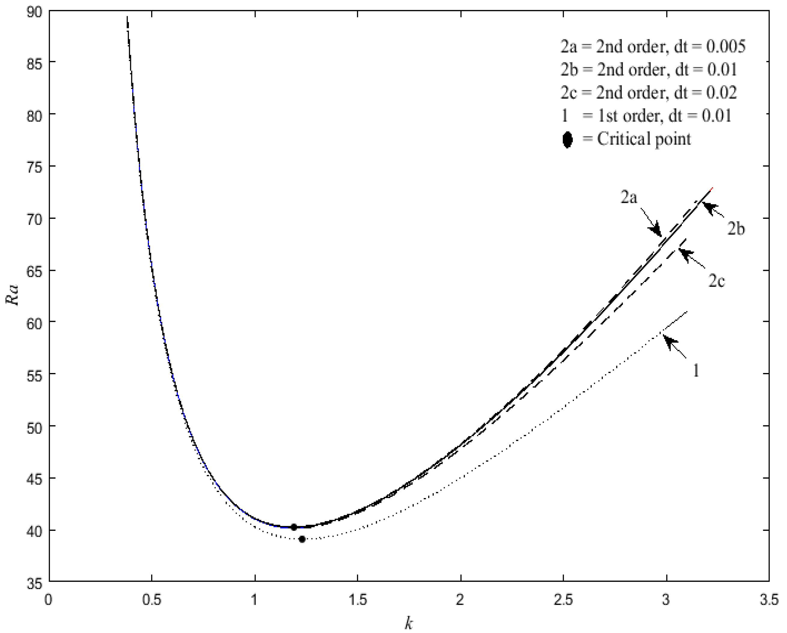
Figure 2 shows the neutral curve as computed by each method and, for the second order method, for three different timesteps. Even graphically it is clear that the accuracy of the first order method is unacceptably poor.
The shape of the neutral curve has the same qualitative features as that of the Darcy-Bénard problem in that it has a well-defined single minimum (which is marked by the solid circle in Figure 2 and Ra grows in an unbounded fashion as k reduces to zero or as k increases. But of most interest is the minimum of the neutral curve, and Table 2 gives this value as obtained using the different methods and timesteps. Once more a detailed analysis of these values shows that they reflect fully the order of accuracy that was used. The use of Richardson’s extrapolation on the Order 2 data yields the following as the values of the critical parameters:
where, if there is any error in the presented data, then we would expect at most a change of 1 in the last displayed decimal place.
kc = 1.1878, Rac = 40.2889,
5.4. Disturbance Profiles
While undertaking the numerical simulations, quantities other than the amplitude (as defined in Equation (14)) were monitored. If the values of fmax and fmin were to be plotted, then it will be clear that the disturbance has a period of 2, even though the basic state has a period of 1. Indeed it was found that fmax (t) = fmin (t + 1) for all t. Even more clearly, the gradient of the reduced temperature disturbance, gʹ(t), has a period of 2. It is therefore of great interest to determine physically why this should arise.
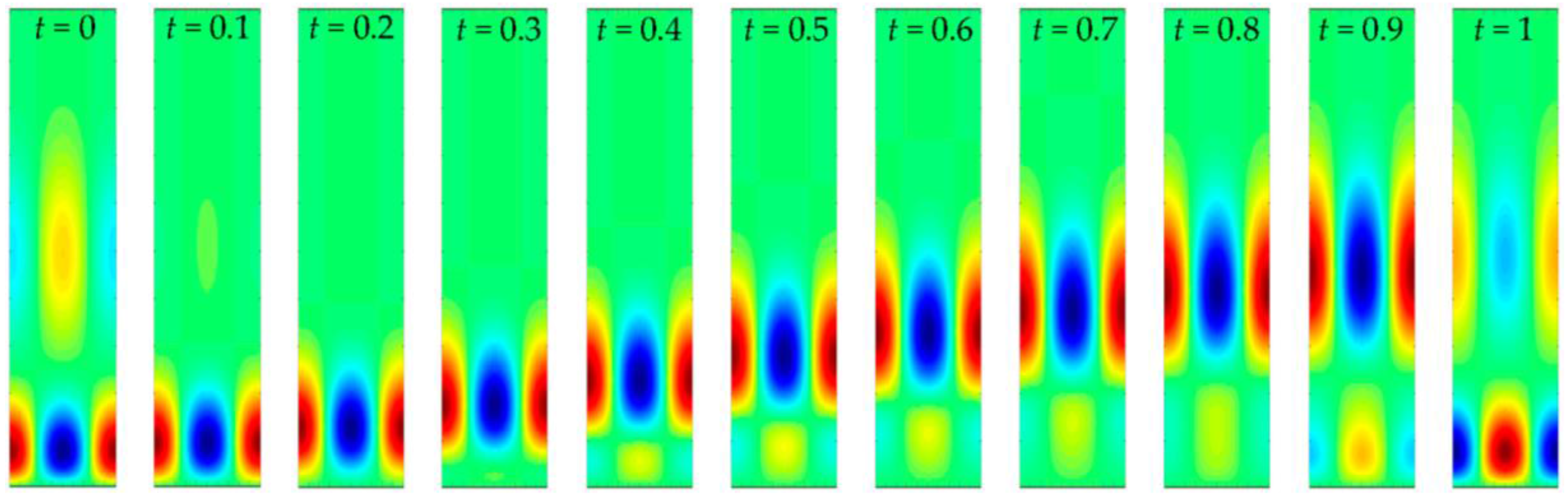
The disturbance temperature fields in the (x,y)-plane were created using Equation (12b) and isotherms were plotted at discrete intervals of time over one period; these are displayed in Figure 3. Red denotes that the fluid is hotter than the background basic state, while blue denotes that it is cooler. Light green corresponds to a vanishingly small disturbance. In each frame the colours are scaled between ±|Θ|max, in order to indicate clearly where the disturbances are concentrated at each instant of time; the values of ±|Θ|max may be found in Table 3. It is also worth noting that the associated streamfunction corresponds (for t = 0) to two whole counter-rotating cells centred in the vertical direction roughly where the temperature disturbances are.
The basic temperature field consists of a sequence of regions, one above another, which are characterised by having temperature gradients of alternating signs. When the sign is negative, then that region is potentially thermoconvectively unstable, but whether or not a local disturbance grows will depend on the value of a local Rayleigh number which may be defined in terms of (i) the height of the potentially unstable region and (ii) its associated temperature drop. Given that t = 0 corresponds to when the boundary is at its hottest, and therefore the porous medium is at its most susceptible to convective instability, it is not surprising that the thermal disturbance is centred close to the boundary.
For a short period of time after t = 0, the local Rayleigh number, which is reducing in magnitude, will be large enough to sustain further growth of the disturbance (see the amplitudes given in Table 3). In this interval of time, the lower boundary is cooling, and therefore the lowest potentially unstable region rises away from the surface, and the disturbance follows its progress (see Figure 3). Eventually the local Rayleigh number becomes too small and the disturbance begins to decay. In the meantime, the main convective cells have risen sufficiently far from the bounding surface that they have generated cells with the opposite circulation below them, i.e., an anticlockwise cell will generate clockwise cell below it and vice versa; it is these latter cells that then begin to grow as t approaches 1 and a new unstable region is then being born. Being of the opposite circulation, it means the upward flow that exists on the left hand side of t = 0 frame in Figure 3 and that drags warm fluid upwards, is replaced by a downward flow on the left hand side of the t = 1 frame that drags cold fluid from above. Another reversal of direction is then obtained once t increases by another unit, and hence the natural period for the disturbance is double that of the basic state.
Cellular patterns that have risen above z = 5 decay extremely rapidly since the basic temperature field is almost perfectly uniform at this height.
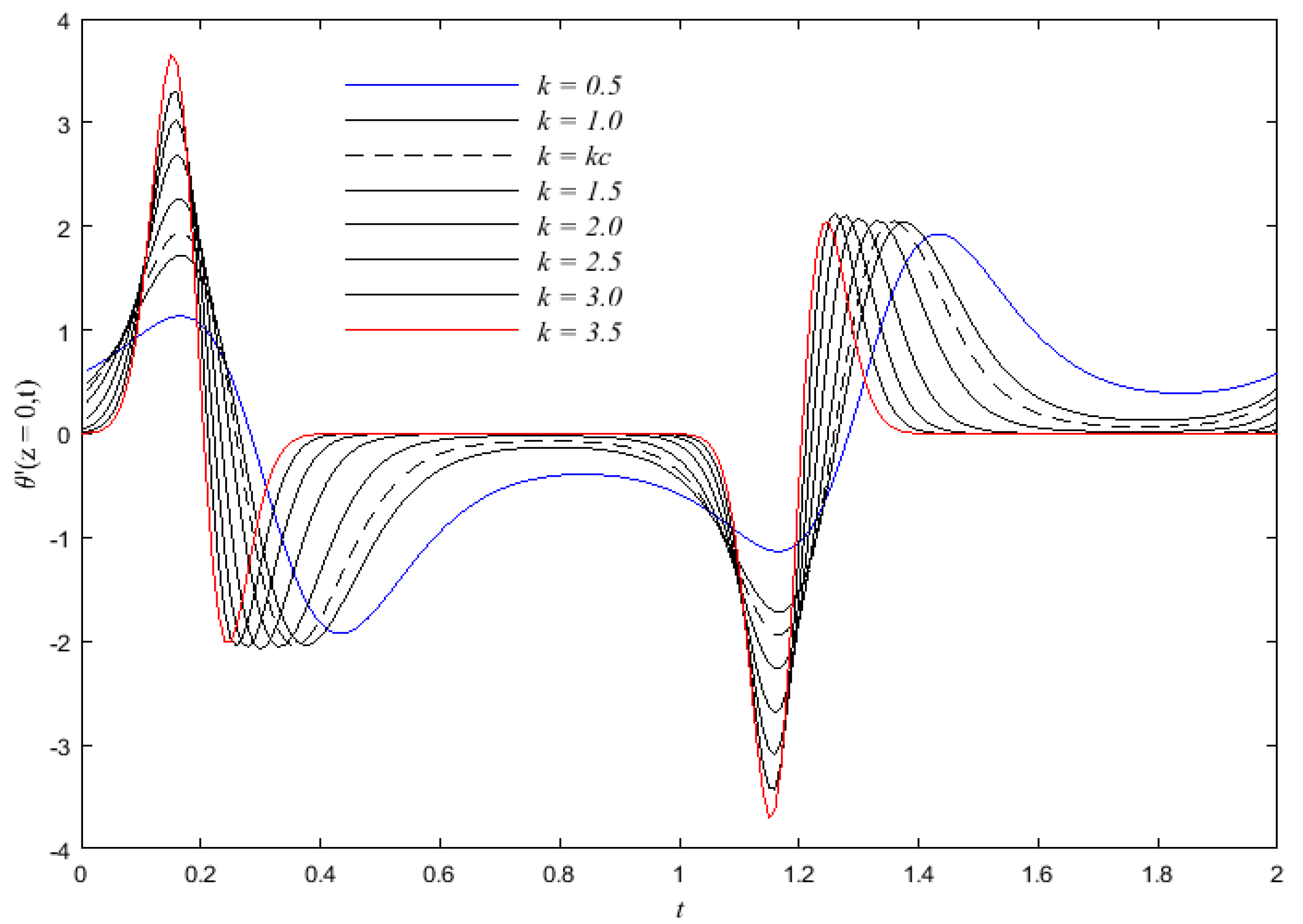
An alternative view is provided by Figure 4 that shows the values of gʹ(z = 0) as a function of time over two periods. The above comments about the period of growth of the disturbance are seen clearly, and this period is almost independent of the chosen wavenumber. However, the surface rate of heat transfer is then dominated by the behaviour of the disturbance at the surface, rather than within the potentially unstable region, which is now above the surface. However, growth in the magnitude of gʹ(z = 0) begins once t passes 0.75, which is when the surface temperature starts to rise again above zero. In the range 1 < t < 2 it is very evident that the surface rate of heat transfer has exactly the opposite sign from that of the first unit period.
We also note that, for the larger values of k, the critical value of Ra is also larger, which means that both the growth and decay phases are more precipitous. This results in a much larger ratio between the maximum disturbance magnitude over a period and the minimum magnitude. In Figure 4 this results in quite a long apparently quiescent phase during the interval of time from t = 0.4 and t = 1.
6. Conclusions
In this work, the onset of convection for a semi-infinite porous domain with a time-varying boundary temperature has been determined by using a numerical linear stability analysis. A Fortran code consisting of the Keller box method was written and internally validated, and onset criteria were obtained by (i) solving the time-evolution of the disturbances; and (ii) iterating towards the value of Ra, which corresponds to zero growth over one forcing period. The computational results showed that the second order method is substantially more accurate than the first order method in absolute terms.
The neutral curve was computed and the critical Darcy-Rayleigh number and the associated wavenumber were both computed to four decimal places; these values are Rac = 40.2889 and kc = 1.1878. Alongside the growth and decay of the disturbance over one forcing period, it was found that disturbances, having been generated at the bounding surface when it is relatively warm, then rise away from the surface and follow the motion of the potentially unstable regions of the basic state. This latter provides the mechanism for cells to reverse direction after one period, and it yields a disturbance that has double the forcing period, a subharmonic instability.
Acknowledgments
The first-named author (Biliana Bidin) would like to thank the Ministry of Higher Education Malaysia (MOHE), particularly the University Malaysia Perlis (UniMAP), for the scholarship which enabled her undertake this work at the University of Bath, UK.
Author Contributions
Biliana Bidin undertook this research as part of her Ph.D. studies and D. Andrew S. Rees supervised the work and assisted with the preparation of the manuscript.
Conflicts of Interest
The authors declare no conflict of interest.
Abbreviations
| f | reduced streamfunction |
| g | reduced temperature |
| gravity | |
| k | wavenumber |
| kc | critical wavenumber |
| K | permeability |
| L | length scale |
| p | pressure |
| pressure (dimensional) | |
| Ra | Darcy-Rayleigh number |
| Rac | critical Darcy-Rayleigh number |
| t | time |
| T | temperature (dimensional) |
| T∞ | temperature (ambient) |
| Tw | temperature (wall) |
| u | velocity in x-direction |
| velocity in x-direction (dimensional) | |
| w | velocity in z-direction |
| velocity in z-direction (dimensional) | |
| x | horizontal coordinate |
| horizontal coordinate (dimensional) | |
| z | vertical coordinate |
| vertical coordinate (dimensional) | |
| Greek letters | |
| α | thermal diffusivity |
| β | thermal expansion coefficient |
| ΔT | temperature difference |
| θ | temperature (nondimensional) |
| Θ | temperature disturbance |
| λ | exponential growth rate |
| μ | dynamic viscosity |
| ρ | reference density |
| σ | heat capacity ratio |
| ψ | streamfunction |
| Ψ | streamfunction disturbance |
| ω | thermal forcing frequency |
References
- Horton, C.W.; Rogers, F.T. Convection currents in a porous medium. J. Appl. Phys. 1945, 16, 367–370. [Google Scholar] [CrossRef]
- Lapwood, E.R. Convection of a fluid in a porous medium. Math. Proc. Camb. Phil. Soc. 1948, 44, 508–521. [Google Scholar] [CrossRef]
- Rees, D.A.S.; Riley, D.S. The effects of boundary imperfections on convection in a saturated porous layer: Near-resonant wavelength excitation. J. Fluid Mech. 1989, 199, 133–154. [Google Scholar] [CrossRef]
- Newell, A.C.; Whitehead, J.C. Finite bandwidth, finite amplitude convection. J. Fluid Mech. 1969, 38, 279–303. [Google Scholar] [CrossRef]
- Nield, D.A. Onset of thermohaline convection in a porous medium. Water Resour. Res. 1968, 11, 553–560. [Google Scholar] [CrossRef]
- McKibbin, R.; O’Sullivan, M.J. Onset of convection in a layered porous medium heated from below. J. Fluid Mech. 1980, 96, 375–393. [Google Scholar] [CrossRef]
- Rees, D.A.S.; Riley, D.S. The three-dimensional stability of finite-amplitude convection in a layered porous medium heated from below. J. Fluid Mech. 1990, 211, 437–461. [Google Scholar] [CrossRef]
- Sutton, F.M. Onset of convection in a porous channel with net through flow. Phys. Fluids 1970, 13, 1931–1934. [Google Scholar] [CrossRef]
- Pieters, G.J.M.; Schuttelaars, H.M. On the nonlinear dynamics of a saline boundary layer formed by throughflow near the surface of a porous medium. Phys. D 2008, 237, 3075–3088. [Google Scholar] [CrossRef]
- Rees, D.A.S. The onset and nonlinear development of vortex instabilities in a horizontal forced convection boundary layer with uniform surface suction. Transp. Porous Media 2009, 77, 243–265. [Google Scholar] [CrossRef]
- Elder, J.W. Transient convection in a porous medium. J. Fluid Mech. 1967, 27, 609–623. [Google Scholar] [CrossRef]
- Caltagirone, J.P. Stability of a saturated porous layer subject to a sudden rise in surface temperature: Comparison between the linear and energy methods. Q. J. Mech. Appl. Math. 1980, 33, 47–58. [Google Scholar] [CrossRef]
- Wooding, R.A.; Tyler, S.W.; White, I. Convection in groundwater below an evaporating salt lake: 1. Onset of instability. Water Res. Res. 1997, 33, 1199–1217. [Google Scholar] [CrossRef]
- Kim, M.C.; Kim, S.; Chung, B.J.; Choi, C.K. Convective instability in a horizontal porous layer saturated with oil and a layer of gas underlying it. Int. Comm. Heat Mass Transfer 2003, 30, 225–234. [Google Scholar] [CrossRef]
- Riaz, A.; Hesse, M.; Tchelepi, H.A.; Orr, F.M. Onset of convection in a gravitationally unstable diffusive boundary layer in porous media. J. Fluid Mech. 2006, 548, 87–111. [Google Scholar] [CrossRef]
- Selim, A.; Rees, D.A.S. The stability of a developing thermal front in a porous medium. I Linear theory. J. Porous Media 2007, 10, 1–15. [Google Scholar] [CrossRef]
- Selim, A.; Rees, D.A.S. The stability of a developing thermal front in a porous medium. II Nonlinear theory. J. Porous Media 2007, 10, 17–23. [Google Scholar] [CrossRef]
- Selim, A.; Rees, D.A.S. The stability of a developing thermal front in a porous medium. III Subharmonic instabilities. J. Porous Media 2010, 13, 1039–1058. [Google Scholar] [CrossRef]
- Selim, A.; Rees, D.A.S. Linear and nonlinear evolution of isolated disturbances in a growing thermal boundary layer in porous media. In Proceedings of the Third International Conference on Porous Media and Its Applications in Science, Engineering and Industry, Montecatini, Italy, 20–25 June 2010; pp. 47–52.
- Noghrehabadi, A.; Rees, D.A.S.; Bassom, A.P. Linear stability of a developing thermal front induced by a constant heat flux. Transp. Porous Media 2013, 99, 493–513. [Google Scholar] [CrossRef]
- Rees, D.A.S.; Selim, A.; Ennis-King, J.P. The instability of unsteady boundary layers in porous media. In Emerging Topics in Heat and Mass Transfer in Porous Media; Vadász, P., Ed.; Springer: Berlin, Germany, 2008; pp. 85–110. [Google Scholar]
- Farrow, D.E.; Patterson, J.C. On the response of a reservoir system to diurnal heating and cooling. J. Fluid Mech. 1993, 246, 143–161. [Google Scholar] [CrossRef]
- Lei, C.W.; Patterson, J.C. Natural convection induced by diurnal heating and cooling in a reservoir with slowly varying topography. JSME Int. J. Ser. B 2006, 49, 605–615. [Google Scholar] [CrossRef]
- Otto, S.R. On the stability of the flow around an oscillating sphere. J. Fluid Mech. 1992, 239, 47–63. [Google Scholar] [CrossRef]
- Hall, P. On the stability of the unsteady boundary-layer on a cylinder oscillating transversely in a viscous fluid. J. Fluid Mech. 1984, 146, 347–367. [Google Scholar] [CrossRef]
- Blennerhassett, P.J.; Bassom, A.P. The linear stability of flat Stokes layers. J. Fluid Mech. 2002, 464, 393–410. [Google Scholar] [CrossRef]
- May, A.; Bassom, A.P. Nonlinear convection in the boundary layer above a sinusoidally heated flat plate. J. Mech. Appl. Math. 2000, 53, 475–495. [Google Scholar] [CrossRef]
Figure 1.
Depicting the semi-infinite porous medium and the imposed boundary conditions.
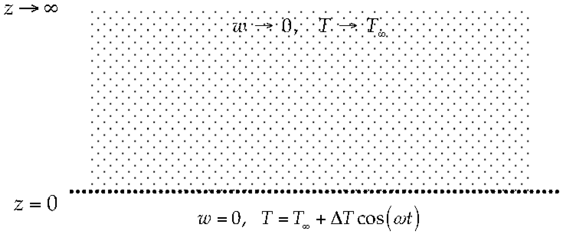
Figure 2.
Neutral curves for the first and second order methods for different timesteps.

Figure 3.
Disturbance isotherms corresponding to critical conditions, namely k = kc and Ra = Rac, and over one forcing period.
Figure 3.
Disturbance isotherms corresponding to critical conditions, namely k = kc and Ra = Rac, and over one forcing period.

Figure 4.
Variation with time of the surface rate of heat transfer of the disturbance over two forcing periods: k = 0.5 (blue); k = 1; k = kc (dashed); k = 1.5; k = 2.0; k = 2.5; k = 3.0; and k = 3.5 (red); where Ra takes the corresponding value from the neutral curve.
Figure 4.
Variation with time of the surface rate of heat transfer of the disturbance over two forcing periods: k = 0.5 (blue); k = 1; k = kc (dashed); k = 1.5; k = 2.0; k = 2.5; k = 3.0; and k = 3.5 (red); where Ra takes the corresponding value from the neutral curve.


| k | Order 1 | Order 2 | ||||
|---|---|---|---|---|---|---|
| dt = 0.02 | dt = 0.01 | dt = 0.005 | dt = 0.02 | dt = 0.01 | dt = 0.005 | |
| 1.0 | 39.5114 | 40.2806 | 40.6998 | 41.0355 | 41.1143 | 41.1341 |
| 2.0 | 42.0992 | 44.9746 | 46.5697 | 47.8046 | 48.1649 | 48.2544 |
| 3.0 | 52.6382 | 59.2835 | 63.3727 | 66.0481 | 67.7715 | 68.1918 |
Table 2.
The dependence of the critical wavenumber and Rayleigh number on the numerical method and the timestep.
| dt | 1st Order Centred | 2nd Order | ||
|---|---|---|---|---|
| kc | Rac | kc | Rac | |
| 0.02 | 1.2912 | 37.9437 | 1.1923 | 40.1568 |
| 0.01 | 1.2356 | 39.1009 | 1.1889 | 40.2560 |
| 0.005 | 1.2109 | 39.6914 | 1.1881 | 40.2807 |
Table 3.
Values of for each thermal disturbance field shown in Figure 3.
| time, t | 0 | 0.1 | 0.2 | 0.3 | 0.4 | 0.5 | 0.6 | 0.7 | 0.8 | 0.9 | 1 |
|---|---|---|---|---|---|---|---|---|---|---|---|
| 0.930 | 4.133 | 14.350 | 22.633 | 19.083 | 11.489 | 5.912 | 2.849 | 1.348 | 0.643 | 0.930 |
© 2016 by the authors; licensee MDPI, Basel, Switzerland. This article is an open access article distributed under the terms and conditions of the Creative Commons Attribution license ( http://creativecommons.org/licenses/by/4.0/).
Share and Cite
MDPI and ACS Style
Bidin, B.; Rees, D.A.S. The Onset of Convection in an Unsteady Thermal Boundary Layer in a Porous Medium. Fluids 2016, 1, 41. https://doi.org/10.3390/fluids1040041
AMA Style
Bidin B, Rees DAS. The Onset of Convection in an Unsteady Thermal Boundary Layer in a Porous Medium. Fluids. 2016; 1(4):41. https://doi.org/10.3390/fluids1040041
Chicago/Turabian StyleBidin, Biliana, and D. Andrew S. Rees. 2016. "The Onset of Convection in an Unsteady Thermal Boundary Layer in a Porous Medium" Fluids 1, no. 4: 41. https://doi.org/10.3390/fluids1040041