Multivariate Functional Time Series Forecasting: Application to Age-Specific Mortality Rates

Abstract

This study considers the forecasting of mortality rates in multiple populations. We propose a model that combines mortality forecasting and functional data analysis (FDA). Under the FDA framework, the mortality curve of each year is assumed to be a smooth function of age. As with most of the functional time series forecasting models, we rely on functional principal component analysis (FPCA) for dimension reduction and further choose a vector error correction model (VECM) to jointly forecast mortality rates in multiple populations. This model incorporates the merits of existing models in that it excludes some of the inherent randomness with the nonparametric smoothing from FDA, and also utilizes the correlation structures between the populations with the use of VECM in mortality models. A nonparametric bootstrap method is also introduced to construct interval forecasts. The usefulness of this model is demonstrated through a series of simulation studies and applications to the age-and sex-specific mortality rates in Switzerland and the Czech Republic. The point forecast errors of several forecasting methods are compared and interval scores are used to evaluate and compare the interval forecasts. Our model provides improved forecast accuracy in most cases.

1. Introduction

Most countries around the world have seen steady decreases in mortality rates in recent years, which also come with aging populations. Policy makers from both insurance companies and government departments seek more accurate modeling and forecasting of the mortality rates. The renowned Lee–Carter model [1] is a benchmark in mortality modeling. Their model was the first to decompose mortality rates into one component, age, and the other component, time, using singular value decomposition. Since then, many extensions have been made based on the Lee–Carter model. For instance, Booth et al. [2] address the non-linearity problem in the time component. Koissi et al. [3] propose a bootstrapped confidence interval for forecasts. Renshaw and Haberman [4] introduce the age-period-cohort model that incorporates the cohort effect in mortality modeling. Other than the Lee–Carter model, Cairns et al. [5] propose the Cairns–Blake–Dowd (CBD) model that satisfies the new-data-invariant property. Chan et al. [6] use a vector autoregressive integrated moving average (VARIMA) model for the joint forecast of CBD model parameters.

Mortality trends in two or more populations may be correlated, especially between sub-populations in a given population, such as females and males. This calls for a model that makes predictions in several populations simultaneously. We would also expect that the forecasts of similar populations do not diverge over the long run, so coherence between forecasts is a desired property. Carter and Lee [7] examine how mortality rates of female and male populations can be forecast together using only one time-varying component. Li and Lee [8] propose a model with a common factor and a population-specific factor to achieve coherence. Yang and Wang [9] use a vector error correction model (VECM) to model the time-varying factors in multi-populations. Zhou et al. [10] argue that the VECM performs better than the original Lee–Carter and vector autoregressive (VAR) models, and that the assumption of a dominant population is not needed. Danesi et al. [11] compare several multi-population forecasting models and show that the preferred models are those providing a balance between model parsimony and flexibility. These mentioned approaches model mortality rates using raw data without smoothing techniques. In this paper, we propose a model under the functional data analysis (FDA) framework.

In functional data analysis settings (see Ramsay and Silverman [12] for a comprehensive Introduction to FDA), it is assumed that there is an underlying smooth function of age as the mortality rate in each year. Since mortality rates are collected sequentially over time, we use the term functional time series for the data. Let $y_t(x)$ denote the log of the observed mortality rate of age x at year t. Suppose $f_t(x)$ is a underlying smooth function, where $x\in \mathcal{I}$ represents the age continuum defined on a finite interval. In practice, we can only observe functional data on a set of grid points and the data are often contaminated by random noise:

$$\begin{array}{c}\hfill y_t(x_j)=f_t(x_j)+u_{t,j},t=1,\cdots ,n,j=1,\cdots ,p,\end{array}$$

where n denotes the number of years and p denotes the number of discrete data points of age observed for each function. The errors $\{u_{t,j}\}$ are independent and identically distributed (iid) random variables with mean zero and variances ${\sigma }_t^2(x_j)$. Smoothing techniques are thus needed to obtain each function $f_t(x)$ from a set of realizations. Among many others, localized least squares and spline-based smoothing are two of the approaches frequently used (see, for example, [13,14]). We are not the first to use the functional data approach to model mortality rates. Hyndman and Ullah [15] propose a model under the FDA framework, which is robust to outlying years. Chiou and Müller [16] introduce a time-varying eigenfunction to address the cohort effect. Hyndman et al. [17] propose a product–ratio model to achieve coherency in the forecasts of multiple populations.

Our proposed method is illustrated in Section 2 and the Appendices. It can be summarized in four steps:

1)

smooth the observed data in each population;

2)

reduce the dimension of the functions in each population using functional principal component analysis (FPCA) separately;

3)

fit the first set of principal component scores from all populations with VECM. Then, fit the second set of principal component scores with another VECM and so on. Produce forecasts using the fitted VECMs; and

4)

produce forecasts of mortality curves.

Yang and Wang [9] and Zhou et al. [10] also use VECM to model the time-varying factor, namely, the first set of principal component scores. Our model is different in the following three ways. First, the studied object is in an FDA setting. Nonparametric smoothing techniques are used to eliminate extraneous variations or noise in the observed data. Second, as with other Lee–Carter based models, only the first set of principal component scores are used for prediction in [9,10]. For most countries, the fraction of variance explained is not high enough for one time-varying factor to adequately explain the mortality change. Our approach uses more than one set of principal component scores, and we review some of the ways to choose the optimal number of principal component scores. Third, in their previous papers, only point forecasts are calculated, while we use a bootstrap algorithm for constructing interval forecasts. Point and interval forecast accuracies are both considered.

The article is organized as follows: in Section 2, we revisit the existing functional time series models and put forward a new functional time series method using a VECM. In Section 3, we illustrate how the forecast results are evaluated. Simulation experiments are shown in Section 4. In Section 5, real data analyses are conducted using age-and sex-specific mortality rates in Switzerland and the Czech Republic. Concluding remarks are given in Section 6, along with reflections on how the methods presented here can be further extended.

2. Forecasting Models

Let us consider the simultaneous prediction of multivariate functional time series. Consider two populations as an example: $f_t^{(\omega )}(x),\omega =1,2$ are the smoothed log mortality rates of each population. According to (A1) in the Appendices, for a sequence of functional time series $\{f_t^{(\omega )}(x)\}$, each element can be decomposed as:

$$\begin{array}{cc}\hfill f_t^{(\omega )}(x)& ={\mu }^{(\omega )}(x)+\sum _{k=1}^{\infty }{\xi }_{t,k}^{(\omega )}{\varphi }_k^{(\omega )}(x)\hfill \\ & ={\mu }^{(\omega )}(x)+\sum _{k=1}^K{\xi }_{t,k}^{(\omega )}{\varphi }_k^{(\omega )}(x)+e_t^{(\omega )}(x),\hfill \end{array}$$

where $e_t^{(\omega )}(x)$ denotes the model truncation error function that captures the remaining terms. Thus, with functional principal component (FPC) regression, each series of functions are projected onto a $K^{(\omega )}$-dimension space.

The functional time series curves are characterized by the corresponding principal component scores that form a time series of vectors with the dimension $K^{(\omega )}$: ${\mathit{\xi }}_t^{(\omega )}={\left({\xi }_{t,1}^{(\omega )},...,{\xi }_{t,K^{(\omega )}}^{(\omega )}\right)}^{\top }$. To construct h-step-ahead predictions ${\widehat{f}}_{n+h|n}^{(\omega )}$ of the curve, we need to construct predictions for the $K^{(\omega )}$-dimension vectors of the principal component scores; namely, ${\widehat{\mathit{\xi }}}_{n+h|n}^{(\omega )}={\left({\widehat{\xi }}_{(n+h|n),1}^{(\omega )},\cdots ,{\widehat{\xi }}_{(n+h|n),K^{(\omega )}}^{(\omega )}\right)}^{\top },$ with techniques from multivariate time series using covariance structures between multiple populations (see also [18]). The h-step-ahead prediction for $f_{n+h|n}^{(\omega )}$ can then be constructed by forward projection

$$\begin{array}{cc}\hfill {\widehat{f}}_{n+h|n}^{(\omega )}& =\mathrm{E}\left[f_{n+h}^{(\omega )}|f_1^{(\omega )}(x),\cdots ,f_n^{(\omega )}(x)\right]\hfill \\ & ={\widehat{\mu }}^{(\omega )}(x)+{\widehat{\xi }}_{(n+h|n),1}^{(\omega )}{\widehat{\varphi }}_1^{(\omega )}(x)+\cdots +{\widehat{\xi }}_{(n+h|n),K^{(\omega )}}^{(\omega )}{\widehat{\varphi }}_{K^{(\omega )}}^{(\omega )}(x),\omega =1,2.\hfill \end{array}$$

In the following material, we consider four methods for modeling and predicting the principal component scores ${\mathit{\xi }}_{n+h}$, where h denotes a forecast horizon.

2.1. Univariate Autoregressive Integrated Moving Average Model

The FPC scores can be modeled separately as univariate time series using the autoregressive integrated moving average (ARIMA($p,d,q$)) model:

$$\begin{array}{c}\hfill \mathrm{\Phi }(B){(1-B)}^d{\xi }_{t,k}^{(\omega )}=\mathrm{\Theta }(B)w_{t,k}^{(\omega )},k=1,\cdots ,K^{(\omega )},\omega =1,2,\end{array}$$

where B denotes the lag operator, and ${\omega }_{t,k}$ is the white noise. $\mathrm{\Phi }(B)$ denotes the autoregressive part and $\mathrm{\Theta }(B)$ denotes the moving average part. The orders $p,d,q$ can be determined automatically according to either the Akaike information criterion or the Bayesian information criterion value [19]. Then, the maximum likelihood method can be used to estimate the parameters.

This prediction model is efficient in some cases. However, Aue et al. [18] argue that, although the FPC scores have no instantaneous correlation, there may be autocovariance at lags greater than zero. The following model addresses this problem by using a vector time series model for the prediction of each series of FPC scores.

2.2. Vector Autoregressive Model

2.2.1. Model Structure

Now that each function $f_t^{(\omega )}(x)$ is characterized by a $K^{(\omega )}$-dimension vector ${\mathit{\xi }}_t^{(\omega )}$, we can model the ${\mathit{\xi }}_t^{(\omega )}$s using a VAR(p) model:

$$\begin{array}{c}\hfill {\mathit{\xi }}_t^{(\omega )}={\mathit{\upsilon }}^{(\omega )}+{\mathit{A}}_1^{(\omega )}{\mathit{\xi }}_{t-1}^{(\omega )}+\cdots +{\mathit{A}}_p^{(\omega )}{\mathit{\xi }}_{t-p}^{(\omega )}+{\mathit{ϵ}}_t,\end{array}$$

where ${\mathit{A}}^{(\omega )}=\{{\mathit{A}}_1^{(\omega )},\cdots ,{\mathit{A}}_p^{(\omega )}\}$ are fixed $K^{(\omega )}\times K^{(\omega )}$ coefficient matrices and $\{{\mathit{ϵ}}_t\}$ form a sequence of iid random $K^{(\omega )}$-vectors with a zero mean vector. There are many approaches to estimating the VAR model parameters in [20] including multivariate least squares estimation, Yule–Walker estimation and maximum likelihood estimation.

The VAR model seeks to make use of the valuable information hidden in the data that may have been lost by depending only on univariate models. However, the model does not fully take into account the common covariance structures between the populations.

2.2.2. Relationship between the Functional Autoregressive and Vector Autoregressive Models

As mentioned in the Introduction, Bosq [21] proposes functional autoregressive (FAR) models for functional time series data. Although the computations for FAR(p) models are challenging, if not unfeasible, one exception is FAR(1), which takes the form of:

$$\begin{array}{c}\hfill f_t=\mathrm{\Psi }(f_{t-1})+{ϵ}_t,\end{array}$$

(1)

where $\mathrm{\Psi }:\mathcal{H}\to \mathcal{H}$ is a bounded linear operator. However, it can be proven that if a FAR(p) structure is indeed imposed on ($f_t:t\in Z$), then the empirical principal component scores ${\mathit{\xi }}_t$ should approximately follow a VAR(p) model. Let us consider FAR(1) as an example. Apply $\langle ·,{\widehat{\varphi }}_k\rangle$ to both sides of Equation (1) to obtain:

$$\begin{array}{cc}\hfill \langle f_t,{\widehat{\varphi }}_k\rangle & =\langle \mathrm{\Psi }(f_{t-1}),{\widehat{\varphi }}_k\rangle +\langle {ϵ}_t,{\widehat{\varphi }}_k\rangle \hfill \\ & =\sum _{k^{\prime }=1}^{\infty }\langle f_{t-1},{\widehat{\varphi }}_{k^{\prime }}\rangle \langle \mathrm{\Psi }({\widehat{\varphi }}_{k^{\prime }}),{\widehat{\varphi }}_k\rangle +\langle {ϵ}_t,{\widehat{\varphi }}_k\rangle \hfill \\ & =\sum _{k^{\prime }=1}^d\langle f_{t-1},{\widehat{\varphi }}_{k^{\prime }}\rangle \langle \mathrm{\Psi }({\widehat{\varphi }}_{k^{\prime }}),{\widehat{\varphi }}_k\rangle +{\delta }_{t,k},\hfill \end{array}$$

with remainder terms ${\delta }_{t,k}=d_{t,k}+\langle {ϵ}_t,{\widehat{\varphi }}_k\rangle$, where $d_{t,k}={\sum }_{k^{\prime }=d+1}^{\infty }\langle f_{t-1},{\widehat{\varphi }}_{k^{\prime }}\rangle \langle \mathrm{\Psi }({\widehat{\varphi }}_{k^{\prime }}),{\widehat{\varphi }}_k\rangle$.

With matrix notation, we get ${\mathit{\xi }}_t=\mathit{B}{\mathit{\xi }}_{t-1}+{\mathit{\delta }}_t$, for $t=2,\cdots ,n$ where $\mathit{B}\in {\mathbb{R}}^{d\times d}$. This is a VAR(1) model for the estimated principal component scores. In fact, it can be proved that the two models make asymptotically equivalent predictions [18].

2.3. Vector Error Correction Model

The VAR model relies on the assumption of stationarity; however, in many cases, that assumption does not stand. For instance, age-and sex-specific mortality rates over a number of years show persistently varying mean functions. The extension we suggest here uses the VECMs to fit pairs of principal component scores of the two populations. In a VECM, each variable in the vector is non-stationary, but there is some linear combination between the variables that is stationary in the long run. Integrated variables with this property are called co-integrated variables, and the process involving co-integrated variables is called a co-integration process. For more details on VECMs, consult [20].

2.3.1. Fitting a Vector Error Correction Model to Principal Component Scores

For the kth principal component score in the two populations, suppose the two are both first integrated and have a relationship of long-term equilibrium:

$$\begin{array}{c}\hfill {\xi }_{t,k}^{(1)}-\beta {\xi }_{t,k}^{(2)}={\delta }_{t,k},\end{array}$$

where $\beta$ is a constant and ${\delta }_{t,k}$ is a stable process. According to Granger’s Representation Theorem, the following VECM specifications exist for ${\xi }_{t,k}^{(1)}$ and ${\xi }_{t,k}^{(2)}$:

$$\begin{array}{c}\hfill \begin{array}{cc}\hfill \Delta {\xi }_{t,k}^{(1)}& ={\alpha }_1\left({\xi }_{t-1,k}^{(1)}-\beta {\xi }_{t-1,k}^{(2)}\right)+{\gamma }_{1,1}\Delta {\xi }_{t-1,k}^{(1)}+{\gamma }_{1,2}\Delta {\xi }_{t-1,k}^{(2)}+{ϵ}_{t,k}^{(1)},\hfill \\ \hfill \Delta {\xi }_{t,k}^{(2)}& ={\alpha }_2\left({\xi }_{t-1,k}^{(1)}-\beta {\xi }_{t-1,k}^{(2)}\right)+{\gamma }_{2,1}\Delta {\xi }_{t-1,k}^{(1)}+{\gamma }_{2,2}\Delta {\xi }_{t-1,k}^{(2)}+{ϵ}_{t,k}^{(2)},\hfill \end{array}\end{array}$$

(2)

where $k=1,\cdots ,K$, and ${\alpha }_1,{\alpha }_2,{\gamma }_{1,1},{\gamma }_{1,2},{\gamma }_{2,1},{\gamma }_{2,2}$ are the coefficients, ${ϵ}_{t,k}^{(1)}$ and ${ϵ}_{t,k}^{(2)}$ are innovations. Note that further lags of $\Delta {\xi }_{t,k}$’s may also be included.

2.3.2. Estimation

Let us consider the VECM(p) without the deterministic term written in a more compact matrix form:

$$\begin{array}{c}\hfill \Delta {\mathit{\xi }}_k={\mathbf{\Pi }}_k{\mathit{\xi }}_{-1,k}+{\mathbf{\Gamma }}_k\Delta {\mathbf{\Psi }}_k+{\mathit{ϵ}}_k,\end{array}$$

where

$$\begin{array}{c}\Delta {\mathit{\xi }}_k=[\Delta {\mathit{\xi }}_{1,k},\cdots ,\Delta {\mathit{\xi }}_{t,k}],\hfill \\ {\mathit{\xi }}_{-1,k}=[{\mathit{\xi }}_{0,k},\cdots ,{\mathit{\xi }}_{n-1,k}],\hfill \\ {\mathbf{\Gamma }}_k=[{\mathbf{\Gamma }}_{1,k},\cdots ,{\mathbf{\Gamma }}_{p-1,k}],\hfill \end{array}$$

$$\begin{array}{c}\Delta {\mathbf{\Psi }}_k=[\Delta {\mathbf{\Psi }}_{0,k},\cdots ,\Delta {\mathbf{\Psi }}_{n-1,k}]\mathrm{with}\Delta {\mathbf{\Psi }}_{t-1,k}=\left[\begin{array}{c}\Delta {\mathit{\xi }}_{t-1,k}\\ ⋮\\ \Delta {\mathit{\xi }}_{t-p+1,k}\end{array}\right],\hfill \\ {\mathit{ϵ}}_k=[{\mathit{ϵ}}_{1,k},\cdots ,{\mathit{ϵ}}_{t,k}].\hfill \end{array}$$

With this simple form, least squares, generalized least squares and maximum likelihood estimation approaches can be applied. The computation of the model with deterministic terms is equally easy, requiring only minor modifications. Moreover, the asymptotic properties of the parameter estimators are essentially unchanged. For further details, refer to [20]. There is a sequence of tests to determine the lag order, such as the likelihood ratio test. Since our purpose is to make predictions, a selection scheme based on minimizing the forecast mean squared error can be considered.

2.3.3. Expressing a Vector Error Correction Model in a Vector Autoregressive Form

In a matrix notation, the model in Equation (2) can be written as:

$$\begin{array}{c}\hfill \Delta {\mathit{\xi }}_{t,k}=\mathit{\alpha }{\mathit{\beta }}^{\top }{\mathit{\xi }}_{t-1,k}+{\mathbf{\Gamma }}_1\Delta {\mathit{\xi }}_{t-1,k}+{\mathit{ϵ}}_{t,k},\end{array}$$

or

$$\begin{array}{c}\hfill {\mathit{\xi }}_{t,k}-{\mathit{\xi }}_{t-1,k}=\mathit{\alpha }{\mathit{\beta }}^{\top }{\mathit{\xi }}_{t-1,k}+{\mathbf{\Gamma }}_1({\mathit{\xi }}_{t-1,k}-{\mathit{\xi }}_{t-2,k})+{\mathit{ϵ}}_{t,k},\end{array}$$

(3)

where

$$\begin{array}{c}\hfill \mathit{\alpha }=\left[\begin{array}{c}{\alpha }_1\\ {\alpha }_2\end{array}\right],{\mathit{\beta }}^{\top }=\left(\begin{array}{cc}1& \beta \end{array}\right),{\mathbf{\Gamma }}_1=\left[\begin{array}{cc}{\gamma }_{1,1}& {\gamma }_{1,2}\\ {\gamma }_{2,1}& {\gamma }_{2,2}\end{array}\right].\end{array}$$

Rearranging the terms in Equation (3) gives the VAR(2) representation:

$$\begin{array}{c}\hfill {\mathit{\xi }}_{t,k}=({\mathit{I}}_K+{\mathbf{\Gamma }}_1+\mathit{\alpha }{\mathit{\beta }}^{\top }){\mathit{\xi }}_{t-1,k}-{\mathbf{\Gamma }}_1{\mathit{\xi }}_{t-2,k}+{\mathit{ϵ}}_{t,k}.\end{array}$$

Thus, a VECM(1) can be written in a VAR(2) form. When forecasting the scores, it is quite convenient to write the VECM process in the VAR form. The optimal h-step-ahead forecast with a minimal mean squared error is given by the conditional expectation.

2.4. Product–Ratio Model

Coherent forecasting refers to non-divergent forecasting for related populations [8]. It aims to maintain certain structural relationships between the forecasts of related populations. When we model two or more populations, joint modeling plays a very important role in terms of achieving coherency. When modeled separately, forecast functions tend to diverge in the long run. The product–ratio model forecasts the population functions by modeling and forecasting the ratio and product of the populations. Coherence is imposed by constraining the forecast ratio function to stationary time series models. Suppose $f^{(1)}(x)$ and $f^{(2)}(x)$ are the smoothed functions from the two populations to be modeled together, we compute the products and ratios by:

$$\begin{array}{cc}\hfill p_t(x)& =\sqrt{f_t^{(1)}(x)f_t^{(2)}(x)},\hfill \\ \hfill r_t(x)& =\sqrt{f_t^{(1)}(x)/f_t^{(2)}(x)}.\hfill \end{array}$$

The product $\{p_t(x)\}$ and ratio $\{r_t(x)\}$ functions are then decomposed using FPCA and the scores can be modeled separately with a stationary autoregressive moving average (ARMA)($p,q$) [22] in the product functions or an autoregressive fractionally integrated moving average (ARFIMA)($p,d,q$) process [23,24] in the ratio functions, respectively. With the h-step-ahead forecast values for ${\widehat{p}}_{n+h|n}(x)$ and ${\widehat{r}}_{n+h|n}(x)$, the h-step-ahead forecast values for ${\widehat{f}}_{n+h|n}^{(1)}(x)$ and ${\widehat{f}}_{n+h|n}^{(2)}(x)$ can be derived by

$$\begin{array}{cc}\hfill {\widehat{f}}_{n+h|n}^{(1)}(x)& ={\widehat{p}}_{n+h|n}(x){\widehat{r}}_{n+h|n}(x),\hfill \\ \hfill {\widehat{f}}_{n+h|n}^{(2)}(x)& ={\widehat{p}}_{n+h|n}(x)/{\widehat{r}}_{n+h|n}(x).\hfill \end{array}$$

2.5. Bootstrap Prediction Interval

The point forecast itself does not provide information about the uncertainty of prediction. Constructing a prediction interval is an important part of evaluating forecast uncertainty when the full predictive distribution is hard to specify.

The univariate model proposed by [15], discussed in Section 2.1, computes the variance of the predicted function by adding up the variance of each component as well as the estimated error variance. The $(1-\alpha )\times 100\%$ prediction interval is then constructed under the assumption of normality, where $\alpha$ denotes the level of significance. The same approach is used in the product–ratio model; however, when the normality assumption is violated, alternative approaches may be used.

Bootstrapping is used to construct prediction interval in the functional VECM that we propose. There are three sources of uncertainties in the prediction. The first is from the smoothing process. The second is from the remaining terms after the cut-off at K in the principal component regression: ${\sum }_{k=K+1}^n{\xi }_{t,k}{\varphi }_k(x)$. If the correct number of dimensions of K is picked, the residuals can be regarded as independent. The last source of uncertainty is from the prediction of scores. The smoothing errors are generated under the assumption of normality and the other two kinds of errors are bootstrapped. All three uncertainties are added up to construct bootstrapped prediction functions. The steps are summarized in the following algorithm:

1)

Smooth the functions with $y_t^{(\omega )}(x_j)=f_t^{(\omega )}(x_j)+u_t^{(\omega )}(x_j),\omega =1,2$, where $u_t^{(\omega )}$ is the smoothing error with mean zero and estimated variance ${\widehat{\sigma }}_t^2{(x_j)}^{(\omega )},j=1,\cdots ,p$.

2)

Perform FPCA on the smoothed functions $f_t^{(1)}$ and $f_t^{(2)}$ separately, and obtain K pairs of principal component scores ${\mathit{\xi }}_{t,k}={\left({\xi }_{t,k}^{(1)},{\xi }_{t,k}^{(2)}\right)}^{\top }$.

3)

Fit K VECM models to the principal component scores. From the fitted scores ${\widehat{\mathit{\xi }}}_{t,k}$, for $t=1,\cdots ,n$ and $k=1,\cdots ,K$, obtain the fitted functions ${\widehat{\mathit{f}}}_t,={\left({\widehat{f}}_t^{(1)},{\widehat{f}}_t^{(2)}\right)}^{\top }$.

4)

Obtain residuals ${\mathit{e}}_t$ from ${\mathit{e}}_t={\mathit{f}}_t-{\widehat{\mathit{f}}}_t$.

5)

Express the estimated VECM from step 3 in its VAR form: ${\mathit{\xi }}_{t,k}={\widehat{\mathit{A}}}_1{\mathit{\xi }}_{t-1,k}+{\widehat{\mathit{A}}}_2{\mathit{\xi }}_{t-2,k}+{\mathit{ϵ}}_{t,k},$ $t=1,\cdots ,n$ and $k=1,\cdots ,K$. Construct K sets of bootstrap principal component scores time series ${\mathit{\xi }}_{t,k}^{*}={\widehat{\mathit{A}}}_1{\mathit{\xi }}_{t-1,k}^{*}+{\widehat{\mathit{A}}}_2{\mathit{\xi }}_{t-2,k}^{*}+{\mathit{ϵ}}_{t,k}^{*}$, where the error term ${\mathit{ϵ}}_{t,k}^{*}$ is re-sampled with replacement from ${\mathit{ϵ}}_{t,k}$.

6)

Refit a VECM with ${\mathit{\xi }}_{t,k}^{*}$ and make h-step-ahead predictions ${\widehat{\mathit{\xi }}}_{n+h|n}^{*}$ and hence a predicted function ${\widehat{\mathit{f}}}_{n+h|n}^{*}$.

7)

Construct a bootstrapped h-step-ahead prediction for the function by

$$\begin{array}{c}\hfill {\widehat{\mathit{f}}}_{n+h|n}^{**}(x_j)={\widehat{\mathit{f}}}_{n+h|n}^{*}(x_j)+{\mathit{e}}_t^{*}+{\mathit{u}}_t^{*}(x_j),\end{array}$$

where ${\mathit{e}}_t^{*}$ is a re-sampled version of ${\mathit{e}}_t$ from step 4 and ${\mathit{u}}_t^{*}(x_j)$ are generated from a normal distribution with mean $\mathbf{0}$ and variance ${\mathit{\sigma }}_{t,j}^2$, where ${\mathit{\sigma }}_{t,j}^2$ is re-sampled from $\{{\widehat{\mathit{\sigma }}}_{1,j}^2,\cdots ,{\widehat{\mathit{\sigma }}}_{n,j}^2\}$ from step 1).

8)

Repeat steps 5 to 7 many times.

9)

The $(1-\alpha )\times 100\%$ point-wise prediction intervals can be constructed by taking the $\frac{\alpha }{2}\times 100\%$ and $(1-\frac{\alpha }{2})\times 100\%$ quantiles of the bootstrapped samples.

Koissi et al. [3] extend the Lee–Carter model with a bootstrap prediction interval. The prediction interval we suggest in this paper is different from their method. First, we work under a functional framework. This means that there is extra uncertainty from the smoothing step. Second, in both approaches, errors caused by dimension reduction are bootstrapped. Third, after dimension reduction, their paper uses an ARIMA(0, 1, 0) model to fit the time-varying component. There is no need to consider forecast uncertainty since the parameters of the time series are fixed. In our approach, parameters are estimated using the data. We adopt similar ideas from the early work of Masarotto [25] for the bootstrap of the autoregression process. This step can also be further extended to a bootstrap-after-bootstrap prediction interval [26]. To summarize, we incorporate three sources of uncertainties in our prediction interval, whereas Koissi et al. [3] only considers one due to the simplicity of the Lee–Carter model.

3. Forecast Evaluation

We split the data set into a training set and a testing set. The four models are fitted to the data in the training set and predictions are made. The data in the testing set is then used for forecast evaluation. Following the early work by [27], we allocate the first two-thirds of the observations into the training set and the last one-third into the testing set.

We use an expanding window approach. Suppose the size of the full data set is 60. The first 40 functions are modeled and one to 20-step-ahead forecasts are produced. Then, the first 41 functions are used to make one to 19-step-ahead forecasts. The process is iterated by increasing the sample size by one until reaching the end of the data. This produces 20 one-step-ahead forecasts, 19 two-step-ahead forecasts, … and, finally, one 20-step-ahead forecast. The forecast values are compared with the true values of the last 20 functions. Mean absolute prediction errors (MAPE) and mean squared prediction errors (MSPE) are used as measures of point forecast accuracy [11]. For each population, MAPE and MSPE can be calculated as:

$$\begin{array}{c}\hfill \begin{array}{cc}\hfill \mathrm{MAPE}(h)& =\frac{1}{(21-h)\times p}\sum _{\eta =h}^{20}\sum _{j=1}^p|y_{n+\eta }(x_j)-{\widehat{f}}_{n+\eta |n+\eta -h}(x_j)|,\hfill \\ \hfill \mathrm{MSPE}(h)& =\frac{1}{(21-h)\times p}\sum _{\eta =h}^{20}\sum _{j=1}^p{\left[y_{n+\eta }(x_j)-{\widehat{f}}_{n+\eta |n+\eta -h}(x_j)\right]}^2,\hfill \end{array}\end{array}$$

(4)

where ${\widehat{f}}_{n+\eta |n+\eta -h}$ represents the h-step-ahead prediction using the first $n+\eta -h$ years fitted in the model, and $y_{n+\eta }(x_j)$ denotes the true value.

For the interval forecast, coverage rate is a commonly used evaluation standard. However, coverage rate alone does not take into account the width of the prediction interval. Instead, the interval score is an appealing method that combines both a measure of the coverage rate and the width of the prediction interval [28]. If ${\widehat{f}}_{n+h|n}^u$ and ${\widehat{f}}_{n+h|n}^l$ are the upper and lower $(1-\alpha )\times 100\%$ prediction bounds, and $y_{n+h}$ is the realized value, the interval score at point $x_j$ is:

$$\begin{array}{c}\hfill \begin{array}{cc}\hfill S_{\alpha }(x_j)& =\left[{\widehat{f}}_{n+h|n}^u(x_j)-{\widehat{f}}_{n+h|n}^l(x_j)\right]\hfill \\ & +\frac{2}{\alpha }\left[{\widehat{f}}_{n+h|n}^l(x_j)-y_{n+h}(x_j)\right]\mathbb{𝟙}\left\{y_{n+h}(x_j)<{\widehat{f}}_{n+h|n}^l(x_j)\right\}\hfill \\ & +\frac{2}{\alpha }\left[y_{n+h}(x_j)-{\widehat{f}}_{n+h|n}^u(x_j)\right]\mathbb{𝟙}\left\{y_{n+h}(x_j)>{\widehat{f}}_{n+h|n}^u(x_j)\right\},\hfill \end{array}\end{array}$$

(5)

where $\alpha$ is the level of significance, and $\mathbb{𝟙}\{·\}$ is an indicator function. According to this standard, the best predicted interval is the one that gives the smallest interval score. In the functional case here, the point-wise interval scores are computed and the mean over the discretized ages is taken as a score for the whole curve. Then, the score values are averaged across the forecast horizon to get a mean interval score at horizon h:

$$\begin{array}{c}\hfill {\overline{S}}_{\alpha }(h)=\frac{1}{(21-h)\times p}\sum _{\eta =h}^{20}\sum _{j=1}^p{S}_{\alpha }[{\widehat{f}}_{n+\eta |n+\eta -h}^u(x_j),{\widehat{f}}_{n+\eta |n+\eta -h}^l(x_j);y_{n+\eta }(x_j)],\end{array}$$

(6)

where p denotes the number of age groups and h denotes the forecast horizons.

4. Simulation Studies

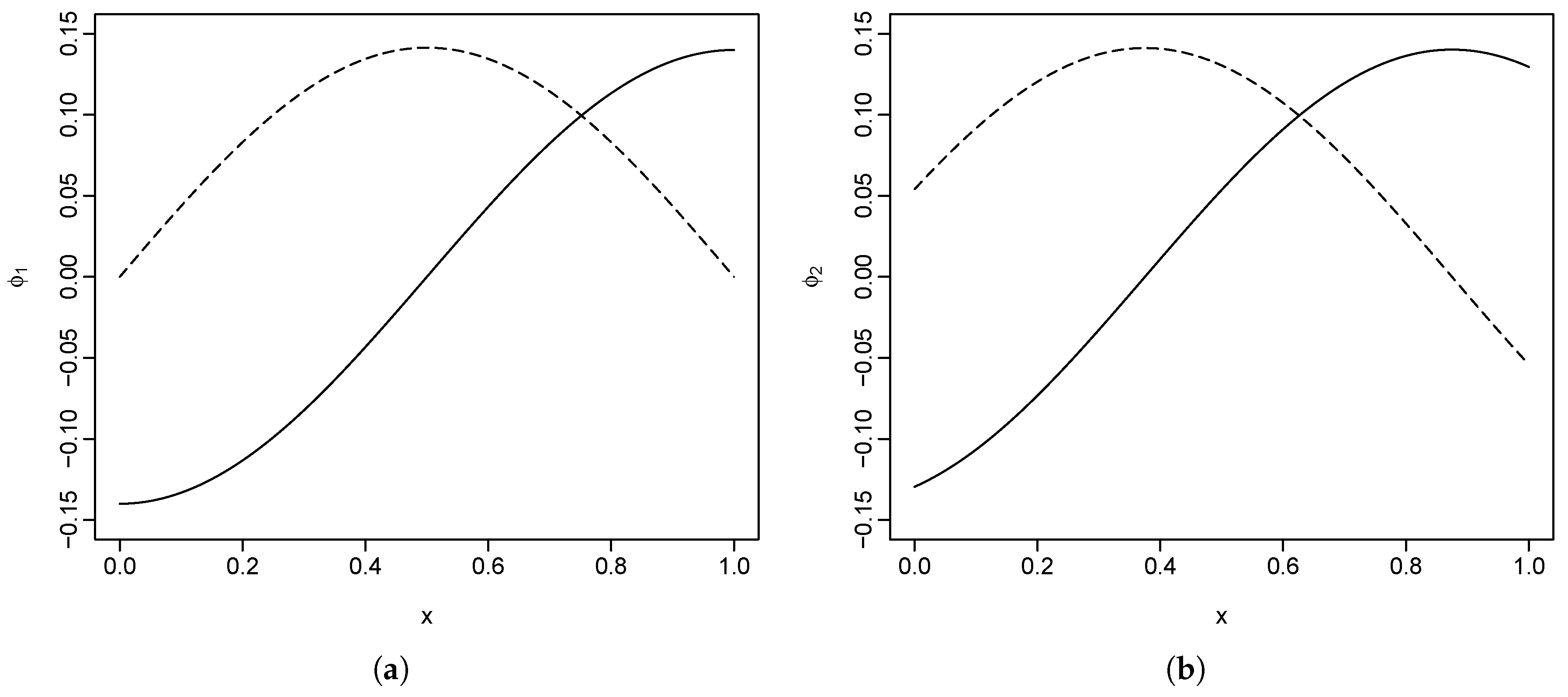
In this section, we report the results from the prediction of simulated non-stationary functional time series using the models discussed in Section 2. We generated two series of correlated populations, each with two orthogonal basis functions. The simulated functions are constructed by

$$\begin{array}{c}\hfill f_t^{(\omega )}(x)={\xi }_{t,1}^{(\omega )}{\varphi }_1^{(\omega )}(x)+{\xi }_{t,2}^{(\omega )}{\varphi }_2^{(\omega )}(x),\omega =1,2.\end{array}$$

(7)

The construction of the basis functions is arbitrary, with the only restriction being that of orthogonality. The two basis functions for the first population we used are ${\varphi }_1^{(1)}(x)=-\cos (\pi x)$ and ${\varphi }_2^{(1)}=\sin (\pi x)$, and, for the second population, these are ${\varphi }_1^{(2)}(x)=-\cos (\pi x+\pi /8)$ and ${\varphi }_2^{(2)}(x)=\sin (\pi x+\pi /8)$, where $x\in [0,1]$. Here, we are using $n=100$ discrete data points for each function. As shown in Figure 1, the basis functions are scaled so that they have an $L_2$ norm of 1.

The principal component scores, or coefficients ${\mathit{\xi }}_{t,k}$, are generated with non-stationary time series models and centered to have a mean of zero. In Section 4.1, we consider the case with co-integration, and, in Section 4.2, we consider the case without co-integration.

4.1. With Co-Integration

We first considered the case where there is a co-integration relationship between the scores of the two populations. Assuming that the principal component scores are first integrated, the two pairs of scores are generated with the following two models:

$$\begin{gathered} \left[\begin{array}{c}\Delta {\xi }_{t,1}^{(1)}\\ \Delta {\xi }_{t,1}^{(2)}\end{array}\right]=\left[\begin{array}{rr}-0.2& 0.4\\ 0.2& -0.4\end{array}\right]\left[\begin{array}{c}{\xi }_{t,1}^{(1)}\\ {\xi }_{t,1}^{(2)}\end{array}\right]+\left[\begin{array}{rr}0.4& 0.3\\ -0.3& -0.4\end{array}\right]\left[\begin{array}{c}\Delta {\xi }_{t-1,1}^{(1)}\\ \Delta {\xi }_{t-1,1}^{(2)}\end{array}\right]+\left[\begin{array}{c}{ϵ}_{t,1}^{(1)}\\ {ϵ}_{t,1}^{(2)}\end{array}\right], \\ \left[\begin{array}{c}\Delta {\xi }_{t,2}^{(1)}\\ \Delta {\xi }_{t,2}^{(2)}\end{array}\right]=\left[\begin{array}{rr}-0.4& 0.4\\ 0.4& -0.4\end{array}\right]\left[\begin{array}{c}{\xi }_{t,2}^{(1)}\\ {\xi }_{t,2}^{(2)}\end{array}\right]+\left[\begin{array}{rr}0.3& -0.2\\ -0.2& 0.3\end{array}\right]\left[\begin{array}{c}\Delta {\xi }_{t-1,2}^{(1)}\\ \Delta {\xi }_{t-1,2}^{(2)}\end{array}\right]+\left[\begin{array}{c}{ϵ}_{t,2}^{(1)}\\ {ϵ}_{t,2}^{(2)}\end{array}\right], \end{gathered}$$

where ${\mathit{ϵ}}_{t,k}$ are innovations that follow a Gaussian distribution with mean zero and variance ${\sigma }_k^2$. To satisfy the condition of decreasing eigenvalues: ${\lambda }_1>{\lambda }_2$, we used ${\sigma }_1^2=0.1$ and ${\sigma }_2^2=0.01$.

It can easily be seen that the long-term equilibrium for the first pair of scores is $-{\xi }_{t,1}^{(1)}+2{\xi }_{t,1}^{(2)}$ and, for the second pair of scores, it is $-{\xi }_{t,2}^{(1)}+{\xi }_{t,2}^{(2)}$.

4.2. Without Co-Integration

When co-integration does not exist, there is no long-term equilibrium between the two sets of scores, but they are still correlated through the coefficient matrix. We assumed that the first integrated scores follow a stable VAR(1) model:

$$\begin{gathered} \left[\begin{array}{c}\Delta {\xi }_{t,1}^{(1)}\\ \Delta {\xi }_{t,1}^{(2)}\end{array}\right]=\left[\begin{array}{rr}0.4& -0.3\\ -0.2& 0.4\end{array}\right]\left[\begin{array}{c}\Delta {\xi }_{t-1,1}^{(1)}\\ \Delta {\xi }_{t-1,1}^{(2)}\end{array}\right]+\left[\begin{array}{c}{ϵ}_{t,1}^{(1)}\\ {ϵ}_{t,1}^{(2)}\end{array}\right], \\ \left[\begin{array}{c}\Delta {\xi }_{t,2}^{(1)}\\ \Delta {\xi }_{t,2}^{(2)}\end{array}\right]=\left[\begin{array}{rr}0.3& 0.1\\ 0.2& 0.5\end{array}\right]\left[\begin{array}{c}\Delta {\xi }_{t-1,2}^{(1)}\\ \Delta {\xi }_{t-1,2}^{(2)}\end{array}\right]+\left[\begin{array}{c}{ϵ}_{t,2}^{(1)}\\ {ϵ}_{t,2}^{(2)}\end{array}\right]. \end{gathered}$$

For a VAR(1) model to be stable, it is required that $\det ({\mathit{I}}_p-{\mathit{A}}_{1}z)=0$ should have all roots outside the unit circle.

4.3. Results

The principal component scores are generated using the aforementioned two models for observations $t=1,\cdots ,60$. Two sets of simulated functions are generated using Equation (7). We performed an FPCA on the two populations separately. The estimated principal component scores are then modeled using the univariate model, the VAR model and the VECM.

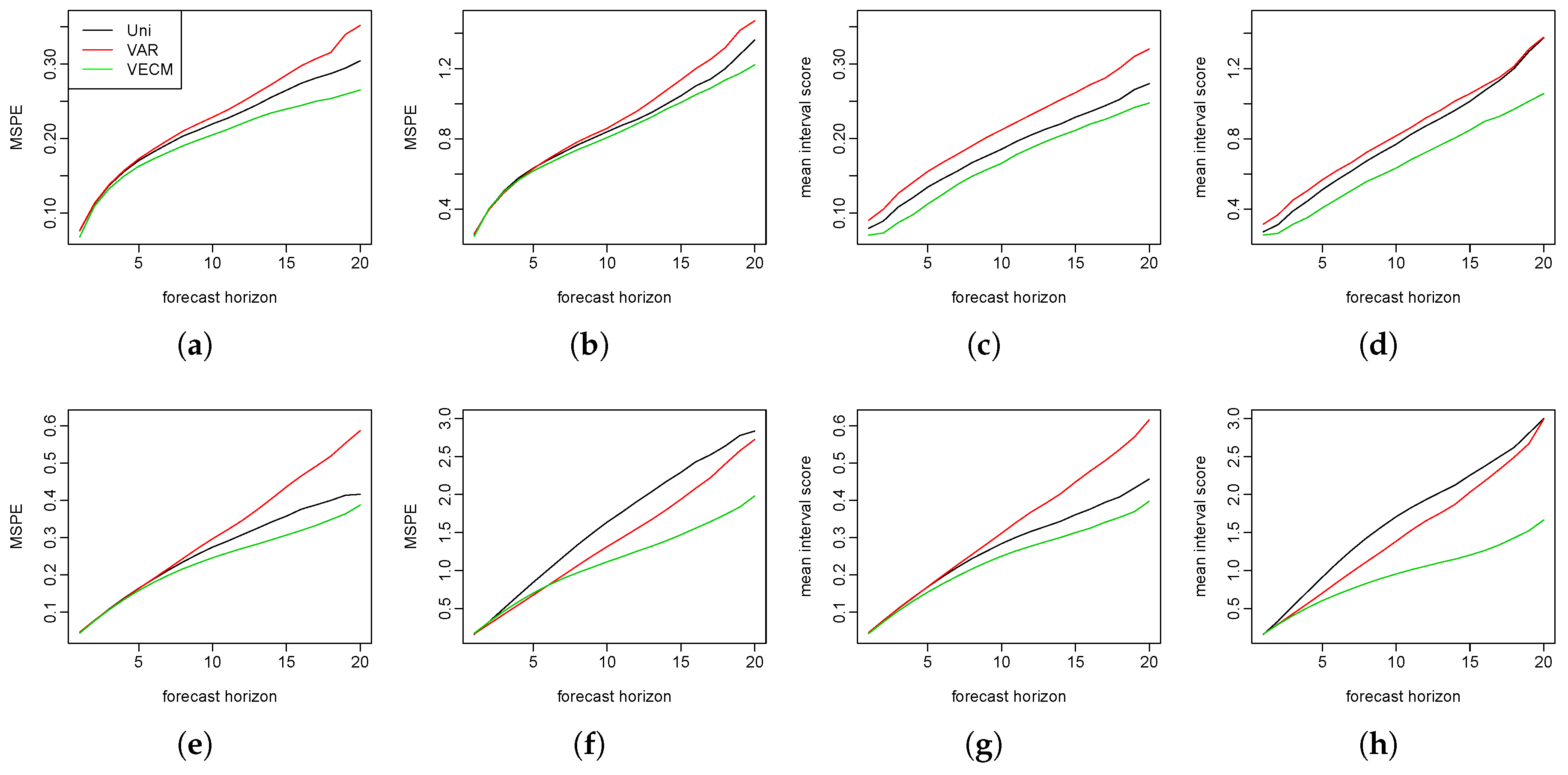
We repeated the simulation procedures 150 times. In each simulation, 500 bootstrap samples are generated to calculate the prediction intervals. We show the MSPE and the mean interval scores at each forecast horizon in Figure 2. The three models performed almost equally well in the short-term forecasts. In the long run, however, the functional VECM produced better predictions than the other two models. This advantage grew bigger as the forecast horizons increased.

5. Empirical Studies

To show that the proposed model outperformed the existing ones using real data, we applied the four models illustrated in Section 2 to the sex-and age-specific mortality rates in Switzerland and the Czech Republic. The observations are yearly mortality curves from ages 0 to 110 years, where the age is treated as the continuum in the rate function. Female and male curves are available from 1908 to 2014 in [29]. We only used data from 1950 to 2014 for our analysis to avoid the possibly abnormal rates before 1950 due to war deaths. With the aim of forecasting, we considered the data before 1950 to be too distant to provide useful information. The data at ages 95 and older are grouped together, in order to avoid problems associated with erratic rates at these ages.

5.1. Swiss Age-Specific Mortality Rates

Figure 3 shows the smoothed log mortality rates for females and males from 1950 to 2014. We use a rainbow plot [30], where the red color represents the curves for more distant years and the purple color represents the curves for more recent years. The curves are smoothed using penalized regression splines with a monotonically increasing constraint after the age of 65 (see [15,31]). Over a span of 65 years, the mortality rates in general have decreased over all ages, with exceptions in the male population at around age 20. Female rates have been slightly lower than male rates over the years.

First, we tested the stationarity of our data set. The Monte Carlo test, in which the null hypothesis is stationarity, was applied to both the male and female populations. We used data from all 65 of the years in our range and performed 5000 Monte Carlo replications [32]. The p-values for the male and female populations were $0.0256$ and $0.0276$, respectively. These small p-values indicated a strong deviation from stationary functional time series.

The first 45 years of data (from 1950 to 1994) were allocated to the training set, and the last 20 years of data from (1995 to 2014) were allocated to the testing set. To choose the order K, we further divided the training set into two groups of 30 and 15 years. The model was fitted to the first 30 years from (1950 to 1979) and forecasts were made for the next 15 years (from 1980 to 1994). In both the VAR model and the functional VECM, K is chosen using:

$$\begin{array}{c}\hfill K=\underset{m}{\mathrm{argmin}}\left\{\frac{1}{15}\sum _{h=1}^{15}\sum _{j=0}^{95}{\left[{\widehat{f}}_{n^{\prime }+h|n^{\prime }}(x_j;m)-y_{n^{\prime }+h}(x_j)\right]}^2\right\},\end{array}$$

where ${\widehat{f}}_{n^{\prime }+h|n^{\prime }}(x_j;m)$ denotes the h-step-ahead forecast based on the first $n^{\prime }=30$ years of data, with m dimensions retained. $y_{n^{\prime }+h}$ denotes the true rate at year $n^{\prime }+h$. This selection scheme led to both the VAR and VECM models with $K=3$ basis functions in this case, which explained $91.20\%$, $4.37\%$ and $1.56\%$ of the variation in the training set, respectively. These add up to $97.13\%$ of the total variances in the training data being explained. In the univariate and the product–ratio models, order $K=6$ is used as in [17,33], where they found that six components would suffice and that having more than six made no difference to the forecasts. With chosen K values, the four models were fitted using an expanding window approach (as explained in Section 3). This produced 20 one-step-ahead forecasts, 19 two-step-ahead forecasts… and, finally, one 20-step-ahead forecast. These forecasts are compared with the holdout data from the years 1995 to 2014. We calculated MAPE and MSPE as point forecast errors using Equation (4).

Table 1. Mean squared prediction error (MSPE) for Swiss female and male rates (the smallest values are highlighted in bold).

h	Female				Male
	UNI	VAR	PR	VECM	UNI	VAR	PR	VECM
1	$0.081$	$0.082$	$0.076$	$\mathbf{0}\mathbf{.}\mathbf{074}$	$0.050$	$\mathbf{0}\mathbf{.}\mathbf{048}$	$0.049$	$0.049$
2	$0.085$	$0.088$	$0.079$	$\mathbf{0}\mathbf{.}\mathbf{075}$	$0.056$	$\mathbf{0}\mathbf{.}\mathbf{052}$	$0.053$	$0.053$
3	$0.090$	$0.094$	$0.084$	$\mathbf{0}\mathbf{.}\mathbf{078}$	$0.065$	$\mathbf{0}\mathbf{.}\mathbf{059}$	$0.060$	$0.060$
4	$0.096$	$0.104$	$0.091$	$\mathbf{0}\mathbf{.}\mathbf{082}$	$0.077$	$\mathbf{0}\mathbf{.}\mathbf{067}$	$0.070$	$0.069$
5	$0.103$	$0.112$	$0.098$	$\mathbf{0}\mathbf{.}\mathbf{086}$	$0.090$	$\mathbf{0}\mathbf{.}\mathbf{078}$	$0.080$	$\mathbf{0}\mathbf{.}\mathbf{078}$
6	$0.109$	$0.119$	$0.107$	$\mathbf{0}\mathbf{.}\mathbf{090}$	$0.107$	$0.093$	$0.093$	$\mathbf{0}\mathbf{.}\mathbf{089}$
7	$0.117$	$0.130$	$0.119$	$\mathbf{0}\mathbf{.}\mathbf{096}$	$0.129$	$0.115$	$0.109$	$\mathbf{0}\mathbf{.}\mathbf{104}$
8	$0.125$	$0.140$	$0.130$	$\mathbf{0}\mathbf{.}\mathbf{102}$	$0.149$	$0.136$	$0.124$	$\mathbf{0}\mathbf{.}\mathbf{119}$
9	$0.136$	$0.151$	$0.145$	$\mathbf{0}\mathbf{.}\mathbf{111}$	$0.171$	$0.160$	$0.139$	$\mathbf{0}\mathbf{.}\mathbf{129}$
10	$0.145$	$0.163$	$0.157$	$\mathbf{0}\mathbf{.}\mathbf{116}$	$0.198$	$0.191$	$0.160$	$\mathbf{0}\mathbf{.}\mathbf{149}$
11	$0.156$	$0.171$	$0.173$	$\mathbf{0}\mathbf{.}\mathbf{125}$	$0.224$	$0.223$	$0.178$	$\mathbf{0}\mathbf{.}\mathbf{162}$
12	$0.167$	$0.186$	$0.195$	$\mathbf{0}\mathbf{.}\mathbf{133}$	$0.261$	$0.269$	$0.206$	$\mathbf{0}\mathbf{.}\mathbf{184}$
13	$0.174$	$0.192$	$0.210$	$\mathbf{0}\mathbf{.}\mathbf{137}$	$0.299$	$0.317$	$0.232$	$\mathbf{0}\mathbf{.}\mathbf{201}$
14	$0.188$	$0.203$	$0.238$	$\mathbf{0}\mathbf{.}\mathbf{145}$	$0.344$	$0.361$	$0.260$	$\mathbf{0}\mathbf{.}\mathbf{213}$
15	$0.183$	$0.209$	$0.254$	$\mathbf{0}\mathbf{.}\mathbf{141}$	$0.396$	$0.414$	$0.293$	$\mathbf{0}\mathbf{.}\mathbf{228}$
16	$0.197$	$0.219$	$0.281$	$\mathbf{0}\mathbf{.}\mathbf{152}$	$0.460$	$0.444$	$0.332$	$\mathbf{0}\mathbf{.}\mathbf{239}$
17	$0.209$	$0.223$	$0.327$	$\mathbf{0}\mathbf{.}\mathbf{164}$	$0.538$	$0.556$	$0.373$	$\mathbf{0}\mathbf{.}\mathbf{251}$
18	$0.209$	$0.233$	$0.354$	$\mathbf{0}\mathbf{.}\mathbf{165}$	$0.649$	$0.652$	$0.416$	$\mathbf{0}\mathbf{.}\mathbf{263}$
19	$0.197$	$0.232$	$0.457$	$\mathbf{0}\mathbf{.}\mathbf{162}$	$0.792$	$0.733$	$0.502$	$\mathbf{0}\mathbf{.}\mathbf{253}$
20	$\mathbf{0}\mathbf{.}\mathbf{144}$	$0.249$	$0.493$	$0.175$	$0.904$	$0.753$	$0.525$	$\mathbf{0}\mathbf{.}\mathbf{270}$
Mean	$0.145$	$0.165$	$0.203$	$\mathbf{0}\mathbf{.}\mathbf{120}$	$0.298$	$0.286$	$0.213$	$\mathbf{0}\mathbf{.}\mathbf{158}$
Median	$0.145$	$0.265$	$0.173$	$\mathbf{0}\mathbf{.}\mathbf{120}$	$0.224$	$0.223$	$0.178$	$\mathbf{0}\mathbf{.}\mathbf{158}$

presents the MSPE of the log mortality rates. The smallest errors at each forecast horizon are highlighted in bold face. For the prediction of the female rates, the proposed functional VECM has proved to make more accurate point forecasts for all forecast horizons except for the 20-step-ahead prediction. It should be noted that there is only one error estimate for the 20-step-ahead forecast, so the error estimate may be quite volatile. The other three approaches are somewhat competitive for the 11-step-ahead forecasts or less. For the longer forecast horizons, the errors of the product–ratio method increase quickly. For the forecasting of male mortality rates, although the VAR model produces slightly smaller values of the forecast errors, there is hardly any difference between the four models in the short term. For long-term predictions, the product–ratio approach performs much better than the univariate and the VAR models, but the VECM still dominates. In fact, the product–ratio model usually outperforms the existing models for the male mortality forecasts, while, for the female mortality forecasts, it is not as accurate. MAPEs of the models followed a similar pattern to the MSPE values and are not shown here.

To examine how the models perform in interval forecasts, Equations (5) and (6) are used to calculate the mean interval scores. We generate 1,000 bootstrap samples in the functional VECM and VAR.

Table 2. Mean interval score (80%) for Swiss female and male rates (the smallest values are highlighted in bold).

h	Female				Male
	UNI	VAR	PR	VECM	UNI	VAR	PR	VECM
1	$1.089$	$1.042$	$0.865$	$\mathbf{0}\mathbf{.}\mathbf{852}$	$0.871$	$0.767$	$\mathbf{0}\mathbf{.}\mathbf{657}$	$0.715$
2	$1.114$	$1.042$	$0.878$	$\mathbf{0}\mathbf{.}\mathbf{864}$	$0.964$	$0.786$	$\mathbf{0}\mathbf{.}\mathbf{699}$	$0.748$
3	$1.153$	$1.059$	$0.909$	$\mathbf{0}\mathbf{.}\mathbf{880}$	$1.088$	$0.852$	$\mathbf{0}\mathbf{.}\mathbf{759}$	$0.791$
4	$1.204$	$1.102$	$0.954$	$\mathbf{0}\mathbf{.}\mathbf{902}$	$1.243$	$0.911$	$\mathbf{0}\mathbf{.}\mathbf{838}$	$0.839$
5	$1.254$	$1.136$	$0.997$	$\mathbf{0}\mathbf{.}\mathbf{926}$	$1.407$	$1.011$	$0.909$	$\mathbf{0}\mathbf{.}\mathbf{887}$
6	$1.306$	$1.169$	$1.046$	$\mathbf{0}\mathbf{.}\mathbf{964}$	$1.594$	$1.134$	$1.005$	$\mathbf{0}\mathbf{.}\mathbf{954}$
7	$1.358$	$1.234$	$1.113$	$\mathbf{0}\mathbf{.}\mathbf{996}$	$1.789$	$1.289$	$1.113$	$\mathbf{1}\mathbf{.}\mathbf{059}$
8	$1.413$	$1.276$	$1.166$	$\mathbf{1}\mathbf{.}\mathbf{026}$	$1.969$	$1.430$	$\mathbf{1}\mathbf{.}\mathbf{190}$	$1.133$
9	$1.483$	$1.349$	$1.241$	$\mathbf{1}\mathbf{.}\mathbf{088}$	$2.134$	$1.587$	$1.282$	$\mathbf{1}\mathbf{.}\mathbf{204}$
10	$1.532$	$1.426$	$1.287$	$\mathbf{1}\mathbf{.}\mathbf{113}$	$2.326$	$1.798$	$1.388$	$\mathbf{1}\mathbf{.}\mathbf{338}$
11	$1.608$	$1.479$	$1.358$	$\mathbf{1}\mathbf{.}\mathbf{170}$	$2.476$	$2.012$	$1.475$	$\mathbf{1}\mathbf{.}\mathbf{458}$
12	$1.661$	$1.591$	$1.437$	$\mathbf{1}\mathbf{.}\mathbf{209}$	$2.655$	$2.303$	$\mathbf{1}\mathbf{.}\mathbf{609}$	$1.628$
13	$1.716$	$1.647$	$1.463$	$\mathbf{1}\mathbf{.}\mathbf{237}$	$2.819$	$2.618$	$\mathbf{1}\mathbf{.}\mathbf{706}$	$1.767$
14	$1.766$	$1.723$	$1.540$	$\mathbf{1}\mathbf{.}\mathbf{281}$	$3.001$	$2.892$	$\mathbf{1}\mathbf{.}\mathbf{793}$	$1.891$
15	$1.705$	$1.775$	$1.571$	$\mathbf{1}\mathbf{.}\mathbf{262}$	$3.145$	$3.082$	$1.892$	$1.963$
16	$1.774$	$1.790$	$1.638$	$\mathbf{1}\mathbf{.}\mathbf{304}$	$3.309$	$3.180$	$\mathbf{1}\mathbf{.}\mathbf{957}$	$1.986$
17	$1.852$	$1.860$	$1.760$	$\mathbf{1}\mathbf{.}\mathbf{352}$	$3.521$	$3.692$	$2.041$	$\mathbf{2}\mathbf{.}\mathbf{011}$
18	$1.819$	$1.884$	$1.767$	$\mathbf{1}\mathbf{.}\mathbf{368}$	$3.632$	$4.148$	$\mathbf{2}\mathbf{.}\mathbf{036}$	$2.051$
19	$1.795$	$1.986$	$1.941$	$\mathbf{1}\mathbf{.}\mathbf{360}$	$3.683$	$4.254$	$2.175$	$\mathbf{1}\mathbf{.}\mathbf{974}$
20	$1.679$	$2.347$	$2.176$	$\mathbf{1}\mathbf{.}\mathbf{398}$	$3.873$	$3.595$	$2.375$	$\mathbf{1}\mathbf{.}\mathbf{978}$
Mean	$1.514$	$1.496$	$1.355$	$\mathbf{1}\mathbf{.}\mathbf{128}$	$2.375$	$2.167$	$1.445$	$\mathbf{1}\mathbf{.}\mathbf{419}$
Median	$1.532$	$1.479$	$1.355$	$\mathbf{1}\mathbf{.}\mathbf{128}$	$2.375$	$2.012$	$1.445$	$\mathbf{1}\mathbf{.}\mathbf{419}$

shows the mean interval scores. The $80\%$ prediction intervals are produced using the four different approaches. As explained earlier, smaller mean interval score values indicate better interval predictions. For the female forecasts, functional VECM makes superior interval predictions at all forecast steps, while, for the male forecasts, the product–ratio model and VECM are very competitive, with the latter having a minor advantage for the mean value.

5.2. Czech Republic Age-Specific Mortality Rates

We have also applied the four models to other countries, such as the Czech Republic, to show that the proposed functional VECM does not only work in the case of the Swiss mortality rates. The raw data are grouped and smoothed as was done for the Swiss data. $K=5$ is chosen in the VAR and the VECM, and the proportions of the explained variance are $93.04\%$, $1.99\%$, $1.55\%$, $1.18\%$, and $0.79\%$ respectively, which add up to $98.55\%$ of the total variance explained. Figure 4 shows the MSPE and mean interval scores for the point and interval forecast evaluations. In order to compare with the VECM model in the literature, we also try fitting only the first set of principal component scores, shown in the figure by VECM*. Among all five models, functional VECM produces better predictions in both the point and interval forecasts. Compared to our model that uses five principal component scores, VECM* produces larger errors, especially in the male forecasts. We consider that an important fraction of information is lost if only the first set of principal component scores is used.

To examine whether or not the differences in the forecast errors are significant, we conduct the Diebold–Mariano test [34]. We use a null hypothesis where the two prediction methods have the same forecast accuracy at each forecast horizon, while the three alternative hypotheses used are that the functional VECM method produces more accurate forecasts than the three other methods. Thus, a small p-value is expected in favor of the alternatives. A squared error loss function is used and the p-values for one-sided tests are calculated at each forecast horizon, as shown in Figure 5. The p-values are hardly greater than zero at most forecast horizons. Almost all are below $\alpha =0.05$, denoted by the horizontal line, with the exception of the 19- and 20-step-ahead forecasts. We conclude that there is strong evidence that the functional VECM method produces more accurate forecasts than the other three methods for most of the forecast horizons.

In summary, we have applied the proposed functional VECM to modeling female and male mortality rates in Switzerland and the Czech Republic, and proven its advantage in forecasting.

6. Conclusions

We have extended the existing models and introduced a functional VECM for the prediction of multivariate functional time series. Compared to the current forecasting approaches, the proposed method performs well in both simulations and in empirical analyses. An algorithm to generate bootstrap prediction intervals is proposed and the results give superior interval forecasts. The advantage of our method is the result of several factors: (1) the functional VECM model considers the covariance between different groups, rather than modeling the populations separately; (2) it can cope with data where the assumption of stationarity does not hold; (3) the forecast intervals using the proposed algorithm combine three sources of uncertainties. Bootstrapping is used to avoid the assumption of the distribution of the data.

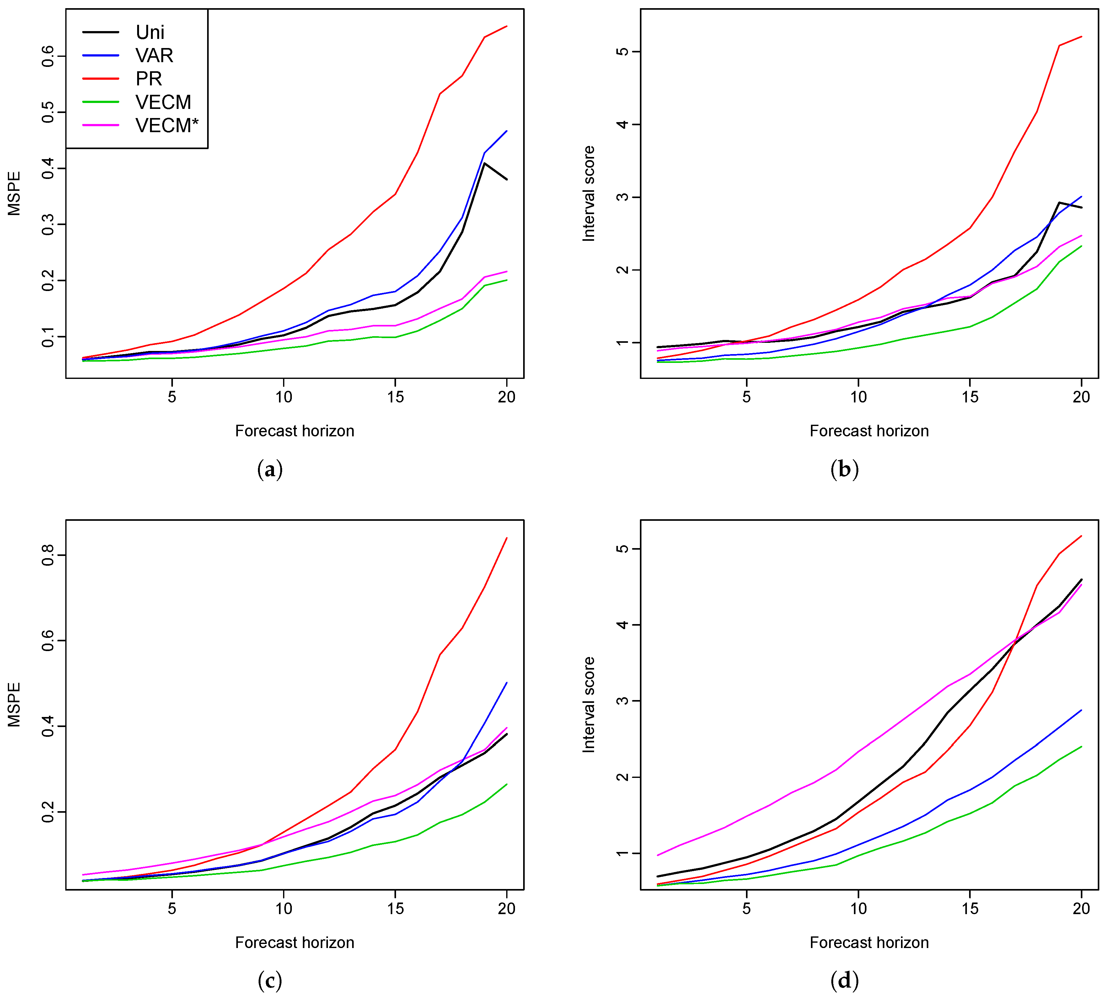
We apply the proposed method as well as the existing methods to the male and female mortality rates in Switzerland and the Czech Republic. The empirical studies provide evidence of the superiority of the functional VECM approach in both the point and interval forecasts, which are evaluated by MAPE, MSPE and interval scores, respectively. Diebold–Mariano test results also show significantly improved forecast accuracy of our model. In most cases, when there is a long-run coherent structure in the male and female mortality rates, functional VECM is preferable. The long-term equilibrium constraint in the functional VECM ensures that divergence does not emerge.

While we use two populations for the illustration of the model and in the empirical analysis, functional VECM can easily be applied to populations with more than two groups. A higher rank of co-integration order may need to be considered and the Johansen test can then be used to determine the rank [35].

In this paper, we have focused on comparing our model with others within functional time series frameworks. There are numerous other mortality models in the literature, and many of them try to deal with multiple populations. Further research is needed to evaluate our model against the performance of these models.

References

1. R.D. Lee, and L.R. Carter. “Modeling and Forecasting U. S. Mortality.” J. Am. Stat. Assoc. 87 (1992): 659–671. [Google Scholar] [CrossRef]
2. H. Booth, J. Maindonald, and L. Smith. “Applying Lee–Carter under conditions of variable mortality decline.” Popul. Stud. 56 (2002): 325–336. [Google Scholar] [CrossRef] [PubMed]
3. M.C. Koissi, A.F. Shapiro, and G. Högnäs. “Evaluating and extending the Lee–Carter model for mortality forecasting: Bootstrap confidence interval.” Insur. Math. Econ. 38 (2006): 1–20. [Google Scholar] [CrossRef]
4. A.E. Renshaw, and S. Haberman. “A cohort-based extension to the Lee–Carter model for mortality reduction factors.” Insur. Math. Econ. 38 (2006): 556–570. [Google Scholar] [CrossRef]
5. A.J.G. Cairns, D. Blake, and K. Dowd. “A two-factor model for stochastic mortality with parameter uncertainty: theory and calibration.” J. Risk Insur. 73 (2006): 687–718. [Google Scholar] [CrossRef]
6. W. Chan, J.S. Li, and J. Li. “The CBD Mortality Indexes: Modeling and Applications.” N. Am. Actualrial J. 18 (2014): 38–58. [Google Scholar] [CrossRef]
7. L.R. Carter, and R.D. Lee. “Modelling and Forecasting US sex differentials in Modeling.” Int. J. Forecast. 8 (1992): 393–411. [Google Scholar] [CrossRef]
8. N. Li, and R. Lee. “Coherent mortality forecasts for a group of populations: An extension of the Lee–Carter method.” Demography 42 (2005): 575–594. [Google Scholar] [CrossRef] [PubMed]
9. S.S. Yang, and C. Wang. “Pricing and securitization of multi-country longevity risk with mortality dependence.” Insur. Math. Econ. 52 (2013): 157–169. [Google Scholar] [CrossRef]
10. R. Zhou, Y. Wang, K. Kaufhold, J.S.H. Li, and K.S. Tan. “Modeling Mortality of Multiple Populations with Vector Error Correction Models: Application to Solvency II.” N. Am. Actuarial J. 18 (2014): 150–167. [Google Scholar] [CrossRef]
11. I.L. Danesi, S. Haberman, and P. Millossovich. “Forecasting mortality in subpopulations using Lee–Carter type models: A comparison.” Insur. Math. Econ. 62 (2015): 151–161. [Google Scholar] [CrossRef]
12. J.O. Ramsay, and J.W. Silverman. Functional Data Analysis. New York, NY, USA: Springer, 2005. [Google Scholar]
13. G. Wahba. “Smoothing noisy data with spline function.” Numer. Math. 24 (1975): 383–393. [Google Scholar] [CrossRef]
14. J. Rice, and B. Silverman. “Estimating the Mean and Covariance Structure Nonparametrically When the Data Are Curves.” J. R. Stat. Soc. Ser. B (Methodol.) 53 (1991): 233–243. [Google Scholar]
15. R.J. Hyndman, and M.S. Ullah. “Robust forecasting of mortality and fertility rates: A fucntional data approach.” Comput. Stat. Data Anal. 51 (2007): 4942–4956. [Google Scholar] [CrossRef]
16. J.M. Chiou, and H.G. Müller. “Linear manifold modelling of multivariate functional data.” J. R. Soc. Stat. Ser. B (Stat. Methodol.) 76 (2014): 605–626. [Google Scholar] [CrossRef]
17. R.J. Hyndman, H. Booth, and F. Yasmeen. “Coherent Mortality Forecasting: The Product-Ratio Method with Functional Time Series Models.” Demography 50 (2013): 261–283. [Google Scholar] [CrossRef] [PubMed]
18. A. Aue, D.D. Norinho, and S. Hörmann. “On the prediction of stationary functional time series.” J. Am. Stat. Assoc. 110 (2015): 378–392. [Google Scholar] [CrossRef]
19. R.J. Hyndman, and Y. Khandakar. “Automatic Time Series Forecasting: The forecast Package for R.” J. Stat. Softw. 27 (2008). [Google Scholar] [CrossRef]
20. H. Lütkepohl. New Introduction to Multiple Time Series Analysis. New York, NY, USA: Springer, 2005. [Google Scholar]
21. D. Bosq. Linear Processes in Function Spaces: Theory and Applications. New York, NY, USA: Springer Science & Business Media, 2012, Volume 149. [Google Scholar]
22. G.E. Box, G.M. Jenkins, G.C. Reinsel, and G.M. Ljung. Time Series Analysis: Forecasting and Control, 5th ed. Hoboken, NJ, USA: John Wiley & Sons, 2015. [Google Scholar]
23. C.W. Granger, and R. Joyeux. “An introduction to long-memory time series models and fractional differencing.” J. Time Ser. Anal. 1 (1980): 15–29. [Google Scholar] [CrossRef]
24. J.R. Hosking. “Fractional differencing.” Biometrika 68 (1981): 165–176. [Google Scholar] [CrossRef]
25. G. Masarotto. “Bootstrap prediction intervals for autoregressions.” Int. J. Forecast. 6 (1990): 229–239. [Google Scholar] [CrossRef]
26. J. Kim. “Bootstrap-after-bootstrap prediction invervals for autoregressive models.” J. Bus. Econ. Stat. 19 (2001): 117–128. [Google Scholar] [CrossRef]
27. J.J. Faraway. “Does data splitting improve prediction? ” Stat. Comput. 26 (2016): 49–60. [Google Scholar] [CrossRef]
28. T. Gneiting, and A.E. Raftery. “Strictly Proper Scoring Rules, Prediction, and Estimation.” J. Am. Stat. Assoc. 102 (2007): 359–378. [Google Scholar] [CrossRef]
29. Human Mortality Database. University of California, Berkeley (USA), and Max Planck Institute for Demographic Research (Germany). 2016. Available online: http://www.mortality.org (accessed on 8 March 2016).
30. R.J. Hyndman, and H.L. Shang. “Rainbow plots, bagplots, and boxplots for functional data.” J. Comput. Graph. Stat. 19 (2010): 29–45. [Google Scholar] [CrossRef]
31. S.N. Wood. “Monotonic smoothing splines fitted by cross validation.” SIAM J. Sci. Comput. 15 (1994): 1126–1133. [Google Scholar] [CrossRef]
32. L. Horvath, P. Kokoszka, and G. Rice. “Testing stationarity of functional time series.” J. Econ. 179 (2014): 66–82. [Google Scholar] [CrossRef]
33. R.J. Hyndman, and H. Booth. “Stochastic population forecasts using functional data models for mortality, fertility and migration.” Int. J. Forecast. 24 (2008): 323–342. [Google Scholar] [CrossRef]
34. F.X. Diebold, and R.S. Mariano. “Comparing predictive accuracy.” J. Bus. Econ. Stat. 13 (1995): 253–263. [Google Scholar] [CrossRef]
35. S. Johansen. “Estimation and Hypothesis Testing of Cointegration Vectors in Gaussian Vector Autoregressive Models.” Econometrica 59 (1991): 1551–1580. [Google Scholar] [CrossRef]
36. J.M. Chiou. “Dynamical functional prediction and classification with application to traffic flow prediction.” Ann. Appl. Stat. 6 (2012): 1588–1614. [Google Scholar] [CrossRef]
37. P. Hall, and C. Vial. “Assessing the finite dimensionality of functional data.” J. R. Stat. Soc. Ser. B (Stat. Methodol.) 68 (2006): 689–705. [Google Scholar] [CrossRef]
38. F. Yao, H. Müller, and J. Wang. “Functional data analysis for sparse longitudinal data.” J. Am. Stat. Assoc. 100 (2005): 577–590. [Google Scholar] [CrossRef]
39. F. Yao, and T.C.M. Lee. “Penalized spline models for functional principal component analysis.” J. R. Stat. Soc. Ser. B (Stat. Methodol.) 68 (2006): 3–25. [Google Scholar] [CrossRef]
40. S. Hörmann, and P. Kokoszka. “Weakly dependent functional data.” Ann. Stat. 38 (2010): 1845–1884. [Google Scholar] [CrossRef]
• Sample Availability: Computational code in R are available upon request from the authors.
Figure 1. Simulated basis functions for the first and second populations. (a) basis functions for population 1; (b) basis functions for population 2.
Risks 05 00021 g001
Figure 2. The first row presents the mean squared prediction error (MSPE) and the mean interval scores for the two populations in a co-integration setting. The second row presents the MSPE and the mean interval scores for the two populations without the co-integration. (a) 1 st population; (b) 2 nd population; (c) 1 st population; (d) 2 nd population; (e) 1 st population; (f) 2 nd population; (g) 1 st population; and (h) 2 nd population.
Risks 05 00021 g002
Figure 3. Smoothed log mortality rates in Switzerland from 1950 to 2014. (a) female population; (b) male population.Short Caption
Risks 05 00021 g003
Figure 4. Czech Republic: forecast errors for female and male mortality rates (MSPE and interval scores are presented). (a) MSPE for female data; (b) mean interval score for female data; (c) MSPE for male data; (d) mean interval score for male data.
Risks 05 00021 g004
Figure 5. Czech Republic: p-values for the three tests comparing a functional VECM to the univariate, VAR, and product–ratio models, respectively (the horizontal line is the default level of significance α = 0 . 05 ). (a) female population; (b) male population.
Risks 05 00021 g005