Shape Similarity Assessment Method for Coastline Generalization

1
Zhengzhou Institute of Surveying and Mapping, Zhengzhou 450000, China
2
School of Marine Science and Technology, Tianjin University, Tianjin 300072, China
*
Author to whom correspondence should be addressed.
ISPRS Int. J. Geo-Inf. 2018, 7(7), 283; https://doi.org/10.3390/ijgi7070283
Submission received: 12 May 2018
/
Revised: 16 July 2018
/
Accepted: 19 July 2018
/
Published: 23 July 2018
Abstract
:Although shape similarity is one fundamental element in coastline generalization quality, its related research is still inadequate. Consistent with the hierarchical pattern of shape recognition, the Dual-side Bend Forest Shape Representation Model is presented by reorganizing the coastline into bilateral bend forests, which are made of continuous root-bends based on Constrained Delaunay Triangulation and Convex Hull. Subsequently, the shape contribution ratio of each level in the model is expressed by its area distribution in the model. Then, the shape similarity assessment is conducted on the model in a top–down layer by layer pattern. Contrast experiments are conducted among the presented method and the Length Ratio, Hausdorff Distance and Turning Function, showing the improvements of the presented method over the others, including (1) the hierarchical shape representation model can distinguish shape features of different layers on dual-side effectively, which is consistent with shape recognition, (2) its usability and stability among coastlines and scales, and (3) it is sensitive to changes in main shape features caused by coastline generalization.
1. Introduction
Coastline is the dynamic boundary between the land and ocean, which is highly related to territorial sea sovereignty, maritime transport, marine resource development, marine science examination, etc. The formation of coastline received a complex effect of many factors such as tides, waves, ocean currents and biological activities, in addition to the general Earth surface processes, making its shape rather irregular and complicated.
In the field of cartography, coastline is usually defined as the boundary reached by average high tide line, which means it belongs to linear features. To fill the multi-scale representation needs [1,2,3], fine-grained coastlines must be transformed into coarse-grained coastline features. In other words, the need for coastline generalization is inevitable. There have been presented a lot of ‘automatic’ linear feature generalization methods in the past decades, such as the Douglas–Peucker algorithm [4], the Li–Openshaw algorithm [5], and the Snake model [6,7].
However, due to the limitation of these automatic generalization methods, and the lack of quality assessment methods for them, artificial intervention is still unavoidable for linear feature generalization, especially for coastlines [8,9,10].
Besides the navigation safety safeguarding principle, one major principle that must be followed during coastline generalization is to preserve the overall shape features [10]. Due to the complexity in shape definition and representation [11,12], almost all of the existing shape similarity theories, methods and models are still imperfect [13,14].
Although the definition of shape is still an open issue, and the relationship between shape similarity and scale is still unclear [15], it is believed that ‘different levels of perception will consider different shapes of a line’ [16]. Therefore, it is of great significance to find an effective method of modelling the shapes of coastlines under different perception levels to evaluate the shape similarity in coastline generalization.
To address this issue, this paper proposes a new method for coastline generalization’s shape similarity assessment. The innovations mainly include: (1) the hierarchical shape representation model: Dual-side Bend Forest is presented which can take shape features on both sides into full consideration and is consistent with shape recognition; (2) the presented method is stable among scales and coastlines; and (3) the presented method is sensitive to change of main shape features caused by coastline generalization.
2. Related Works
For the reasons: (1) the achievements of the coastline’s shape similarity assessment are still not abundant enough, and (2) coastline is a special kind of linear features. This section mainly summarizes related research of general linear features.
The key-point of the shape similarity assessment for a linear feature lies in the parameterization of the linear feature’s shape, namely, the design of the shape representation model (also known as shape descriptor). Recently, most of the achievements about shape representation models have been achieved in geo-sciences, pattern cognition and computer graphics, most of which satisfy the “three-invariance” rule towards affine transformation, namely, the invariance of rotation, translation and scale [17,18].
For any linear feature and its generalized version , the shape similarity degree between them can be represented by:
where are the shape representation models of and , respectively.
Based on the differences in linear feature’s shape representation model, this paper divides all the shape similarity assessment methods into three categories: direct methods, holistic representation-based methods and local representation-based methods.
2.1. Direct Methods
Methods of this category usually attempt to measure the shape difference between two linear features directly without giving a definite representation of the shape, which mainly contain various distance metrics-based methods [19].
2.1.1. Hausdorff Distance
For finite point sets , the Hausdorff distance (HD) between them can be defined as [20]:
while, for line features, as there are infinite points on them, the computation of HD will become extremely complex. Thus, the discrete HD between lines was presented as [21]:
where are the vertices of line features , respectively.
To overcome the drawback of HD that it is too sensitive to outliers, the Modified HD [22] and the Activated Hausdorff Proximity [23] are presented.
Although primitive, the HD and its varieties seem to be available for linear feature shape similarity assessment in many cases. However, as they just focus on the distance feature [24], the result of measuring two intertwined curves will be unreliable.
2.1.2. Fréchet Distance
A linear feature can be represented as: . Thus, for every , every is affine. In other words, is true for all , where is called the length of .
For two curves , the Fréchet distance (FD) between them: is:
Here, are continuous, monotonic increasing functions which meet: .
Although FD has been proved to be more suitable as the distance metrics between linear features [24], it is still unsuitable for massive points due to the massive computation burden of continuous mathematics [24]. Later, a data structure named the free-space diagram [25] was presented to improve the computational efficiency for many methods, including the FD [26,27].
2.2. Holistic Representation-Based Methods
2.2.1. Simple Geometry Parameter-Based Methods
Length is a holistic feature of linear features, which seems to be closely related to shape. From this point of view, the Length Ratio (LR) [28] was presented and has been widely used. The LR uses the total length ratio between two linear features as the parameter to measure their shape similarity. Namely:
where are the total lengths of linear features and , respectively.
Although this method does not meet the three-invariance rule, it is still popular because of its simplicity and ease of implementation.
2.2.2. Complex Geometry Parameter-Based Methods
Unlike methods like LR, some researchers tend to find other parameters that can represent shape features. Famous methods of this kind include Included Angle Chain (IAC) [29], Angle Difference Integral (ADI) [30], and Turning Function (TF) [31], as Table 1 shows.
For their ease of implementation, these methods quickly received much attention and research, and many variants of the TF including Signature Function [32] and Tangent Function [33] were presented. In recent research [34], the TF was mentioned to achieve the best matching result among many methods.
There are many more methods in this categories presented, including: (1) the function-based methods, which are widely used in pattern cognition and image matching, such as Fourier Shape Descriptor [35,36], Wavelet Shape Descriptor [37,38] and SimpliPoly [39]; (2) fractal geometry-based methods [40], which can be used in addressing the influence of generalization of shape features’ variation [41,42,43,44,45]; (3) other holistic methods, which are usually used in computer graphics domain, such as Kullback–Leibler Divergence [46], statistics [47], Shape Context [48], Scale Invariant Feature Transform (SIFT) [49] and Location-Orientation Rotary Descriptor (LORD) [18]. Among these, the Shape Context is regarded the most important method in the 21th century.
2.3. Local Representation-Based Methods
Unlike holistic representation methods, this kind of method first divides the entire linear feature into several parts. Based on the division method, these methods can be divided into two categories.
2.3.1. Critical Point-Based Partition Methods
In the middle of the last century, it was proved that ‘information is further concentrated at points where a contour changes direction most rapidly’ [50]. The linear feature’s shape detection began to focus on critical point detection ever since [51,52,53,54]. The definition of critical point has been constantly updated over time [55]. By now, the critical point of a linear feature should include the curvature discontinuous point, the start/end point, the curvature maximum/minimum point and the inflection point [11].
A review of critical point detection algorithms, which can be used in linear feature generalization, shows that, for (discrete) linear features, the curvature can only be approximated, which is an inherent defect of all the algorithms [56]. Recently, the critical point detection methods have tended to use other metrics to replace curvature, such as Local Length Ratio (LLR) [57]. However, although these varieties eliminated the approximate calculation, they are still sensitive to the points’ spatial distributions since points farther from the neighboring points tend to have a higher probability to be detected as a critical point regardless of its real curvature, which may in turn affect the final result.
2.3.2. Bend-Based Partition Methods
Methods of this category treat linear features as a sequence of ordered bends. As the definition of bend is still controversial, bend division methods are not unique. At the beginning, bends were generated by segmenting the linear feature using certain kinds of feature points [7]. However, the relationship among bends obtained by this method is simple linear adjacency, which means the multi-scale feature of linear feature shape is neglected. Later, the method based on inter-visibility was presented [58]. Until now, the most representative method is the one based on Constrained Delaunay Triangulation (CDT) [54]. The CDT [59] is different from Delaunay Triangulation by adding the linear feature’s segments as constrained edges where the edges of the CDT are not allowed to intersect with.
When generating CDT, one ‘Super Triangle’ that can completely include is firstly generated. Then, is generated upon set using both and ’s edges as constrained edges. After that, every triangle can be classified into four categories to run the ‘triangle stripping trace’ process, as Table 2 shows.
The process of ‘triangle stripping trace’ begins at one Type I triangle, during which the tracker continues to delete the current triangle and enter its neighbors until one Type II triangle is reached. In this process, if the current triangle is a Type III, the tracker will just move to its neighbor. If the current triangle is a Type IV, the tracker will split it in two to continue tracing, thus generating a binary tree structure.
After the whole process, a series of shape parameters (including bend size, direction, average width, depth, coverage region, etc.) for bends can be calculated. For example, as is shown in Figure 1 and Table 3, several geometric characteristic parameters of bend tree are calculated.
However, the method still suffers one main drawback as the entire linear feature is represented by one single bend binary tree, while, in the real world, one linear feature may contain several non-inclusive bends.
As a summary, while the above methods can be used to measure the shape similarity among linear features to some extent, none of these can fully represent the (global) directionality and the (local) basic sinuosity, which is believed to be the two basic dimensions in a linear feature’s shape [16,60]. Meanwhile, mixing several parameters together will: (1) face the weight allocation problem whose solution remains to be experience-driven (e.g., the expert system) and (2) lack a rigorous mathematical basis.
3. Dual-Side Bend Forest-Based Coastline Shape Similarity Assessment Method
The process of assessing the shape similarity of coastlines before and after generalization mainly consists of two parts: (1) the design of coastline’s shape representation model (hereinafter referred to as model), and (2) the shape similarity assessment based on the model.
Considering (1) shape cognition’s hierarchical pattern [61,62] and (2) the special demands (e.g., safety) of coastline generalization [9], to fully represent the coastline’s shape, the model used in the coastline’s shape similarity assessment should consider the following aspects:
1. The hierarchical structure should be provided.
The shape features represented by the model should match our intuitive shape cognition, which means that the model should provide a hierarchical structure [63].
2. The shape feature of both sides should be considered targeted.
The shape feature exists on both sides of the linear feature [64,65,66]. Thus, rather than considering the shape feature of either side, the shapes of both sides should be taken into consideration.
More specifically, as each side of the coastline must be treated pointedly, namely the land side should be expended in general, while the ocean side should be reduced during the generalization process, shape features on each side should be considered targeted.
To satisfy these properties, a hierarchical coastline shape similarity assessment method called a Dual-side Bend-tree Forest shape representation model (DBF) is presented in this section.
3.1. Dual-Side Bend-Tree Forest Shape Representation Model
Considering the specificity of coastline, the positive direction of the coastline is set by making the land side the left side of it. Inspired by [54], this paper also uses the CDT to identify bends to generate DBF, which has the greater ability to represent the continuity and hierarchical pattern of bends along the coastline.
3.1.1. Basic Definitions
As is shown in Figure 2, after the CDT construction, all the edges can be divided into three categories:
1. Constrained edges
Edges of this category are the ones of the coastline, e.g., edges AB, CD.
2. Non-constrained edges
The edges that are newly formed during the CDT construction are defined as non-constrained edges, e.g., edges BD, FN.
3. Convex hull edges
Edges of this category formed the convex boundary of the whole coastline. It is worth mentioning that convex hull edges can be either constrained edges (e.g., AB) or non-constrained edges (e.g., ).
Based on these definitions, bends formed by the coastline and its CDT can be divided as follows:
1. Root-bend
By considering the relationship of regions on the left side and right side of the coastline as ’non-connected’, convex hull edges and constrained edges will divide the whole convex region into several adjacent but non-connected sub-regions, each of which includes one convex hull edge (baseline) and a certain number of constrained and non-constrained edges. These sub-regions are defined as root-bends, as their roles in DBF are the roots of bend binary trees.
2. Flat bend
Root-bends whose convex hull edge belongs to the constrained edges are defined as flat bends. There is only one constrained edge and no non-constrained edge in one flat bend (e.g., root-bend AB on the right side).
3. Non-flat bend
Root-bends whose convex hull edge belongs to the non-constrained edges are defined as non-flat bends. There are at least one non-constrained edge and two constrained edges in one non-flat bend (e.g., root-bend on the right side).
3.1.2. The Generation of Dual-Side Root-Bend Forest
Based on the above definitions, coastline can be divided into several root-bends by using the Algorithm 1, and each root-bend can be classified into either side to generate the dual-side bend forest.
| Algorithm 1 Root-bend classification | |
| 1 | For every convex hull edge in of coastline : |
| 2 | Judge if belongs to the constrained edges: |
| 3 | True: This root-bend is a flat bend |
| 4 | Find triangle in CDT of coastline that includes |
| 5 | Judge the relative location of ’s centroid point (left or right) |
| 6 | Left: Add into the Right-side bend forest list |
| 7 | Right: Add into the Left-side bend forest list |
| 8 | False: This root-bend is a non-flat bend |
| 9 | Find triangle in CDT of coastline that includes |
| 10 | Judge the relative location of ’s centroid point (left or right) |
| 11 | Left: Add into the Left-side bend forest list |
| 12 | Right: Add into the Right-side bend forest list |
3.1.3. The Generation of Hierarchical Bend Tree
The generation of hierarchical bend tree begins with the root-bends’ baselines, as is shown in Algorithm 2.
| Algorithm 2 Bend tree generation | |
| 1 | For each root-bend , if its baseline is a non-constraint edge, mark it as root node. |
| 2 | Find the only Delaunay triangle that includes |
| 3 | Judge the other 2 edges of |
| 4 | Case 1: Both edges are constraint edges: |
| 5 | Algorithm moves to leaf nodes, terminated. |
| 6 | Case 2: At least one edge is non-constraint edge: |
| 7 | Add this edge into child nodes in the tree |
| 8 | Move current baseline to this edge, back to 2 |
| 9 | Else: Algorithm terminated. |
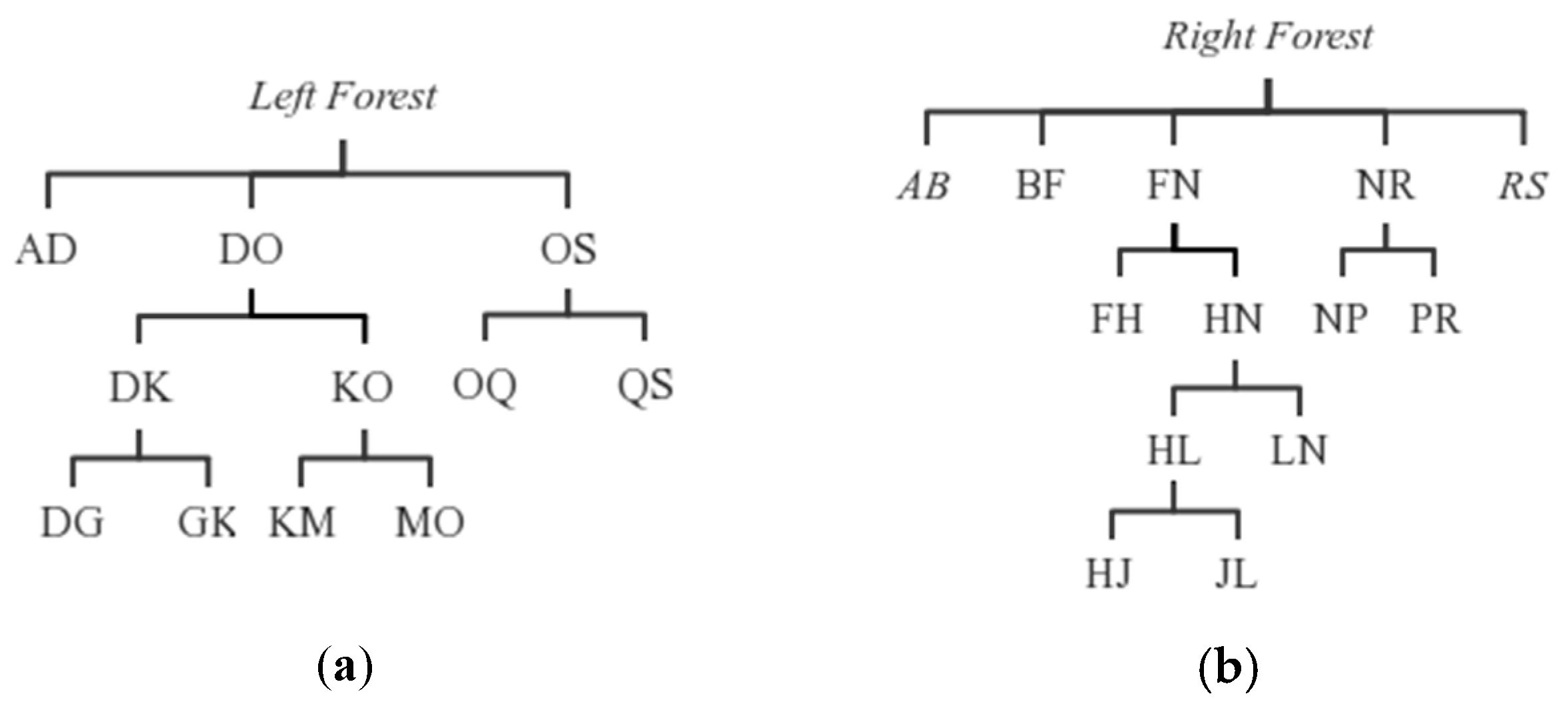
When the algorithm terminates, two forests composed of several bend trees are generated to describe the shape of the coastline (the bend trees of flat bends are empty). Therefore, it is named the Dual-side Bend Forest (DBF). An example of DBF on sample coastline is shown in Figure 3 (the flat bends, AB and RS, are shown in italics).
It is worth mentioning that, as bend consists of several consecutive straight-line segments, which in turn makes up of one pair of nodes, the interval expansion of all nodes is closed in this paper.
Obviously, the DBF mentioned above can: (1) turn the shape of the coastline into a hierarchical structure to meet the coastline’s multi-scale representation need, and (2) ensure the shape representation’s completeness as root-bends on the same side are continuous; thus, the coastline can be reorganized in a layer by layer pattern.
However, as all bends are represented by their baselines, the bends’ shape representation is still lacking by now. Theoretically, to form a none-0 area 2D shape, at least three non-collinear vertices are needed, therefore, to form the shape of any non-flat bend, and, given its baseline, only one more feature point is needed. To ensure the uniqueness of the feature point, the first maximum distance vertex (height point) towards the baseline is selected to represent the bend’s shape. For example, the root-bend on the right side of can be represented by .
3.2. DBF Based Shape Similarity Assessment Method for Coastline Generalization
Based on the DBF shape representation model, a hierarchical shape similarity assessment method: DBF-based Shape Similarity (DBF-SS) is presented to assess the shape similarity degree for coastline generalization.
3.2.1. DBF Based Shape Similarity Assessment Method
Bend’s shape similarity assessment is the basis of coastline’s shape similarity assessment. Considering the coastline’s (1) generalization principles, and (2) spatial location features, the Jaccard similarity coefficient [67] of two reorganized coastlines is used to quantize the shape similarity between them. Namely, shape similarity degree between a pair of reorganized coastlines of the same layer and , , can be calculated by:
3.2.2. Weight Distribution in DBF
The shape area counts in human’s shape cognition. The larger the area of the shape, the greater the degree of its importance. Thus, the overall shape similarity result cannot be obtained by simply adding the shape similarity of layers together. In other words, weights need to be allocated inhomogeneously among layers.
Based on the bend area, a hierarchical weight allocation method is presented. To be specific, the steps are as follows:
- The total weight of the whole area inside the convex hull is set to 1.
- The weights of root-bends are allocated based on their area ratio to the total area of the region inside the convex hull. Namely:
- The weights within each root-bend are allocated follow the order from the root node to the leaf node based on area ratio. Namely, for a pair of sibling nodes whose parent node is , let the weight of be , the weight allocation between will be:
- The weights of every layer are the sum of all the bends in it. Namely, for any layer , its weight will be:
3.2.3. Global Shape Similarity Assessment Method
Consistent with the hierarchical order of shape recognition, the shape similarity index should be calculated in a layer by layer pattern. Based on the above method, the shape similarity degree of two coastlines will be:
where are the reorganized coastlines on of coastlines and , respectively.
4. Experiments
To fully test the performance of the presented method, three widely used shape similarity assessment methods including Length Ratio (LR), Hausdorff Distance (HD) and Turning Function (TF) are implemented to conduct three groups of contrast experiments. All experiments are run on a prototype system built on Python 2.7.13.
(1) Experiments on specific coastlines.
Firstly, two sets of coastlines with different shape features extracted from ENC (Electronic Nautical Chart) sheets downloaded from the NOAA (National Oceanic and Atmospheric Administration) website are used to further evaluate the performance of experimental methods in detail.
(2) Experiments on simulation generalization results.
Secondly, a set of coastlines generalized manually from one coastline is involved to verify the sensitivity of experimental methods on possible quality problems during generalization.
(3) Experiments on global coastline datasets.
Thirdly, experiments are performed on global datasets named the Global Self-consistent Hierarchical High-resolution Shorelines (GSHHS) of three different scales downloaded from NOAA to further verify the applicability of the experimental methods on large datasets.
Specifically, experimental coastlines in this section include: (1) three relatively simple coastline segments: Coastlines 0–2 (referred to as ); (2) a pair of relatively complex coastline segments: Coastlines 3, 4 (referred to as ); (3) a series of coastline segments generalized manually from coastline 4 to simulate different generalization results: Coastlines 5–8 (referred to as ); (4) coastlines extracted from global coastline datasets of three different scales; basic information of these coastlines including vertex number, total length and shape complexity (represented by ) is shown in Table 4, in which the parentheses in the header are the measure units.
4.1. Experiments on Specific Coastlines
The main purpose of this part is to testify to the usability of all the methods among different scales and coastlines in detail. Thus, two groups of coastlines, including one group of coastlines whose shape features are relative simple (Coastlines 0–2) and one group of coastlines whose shape features are relative complex (Coastlines 3, 4), are selected in this part.
4.1.1. Experimental Coastlines
1. Relatively simple coastlines
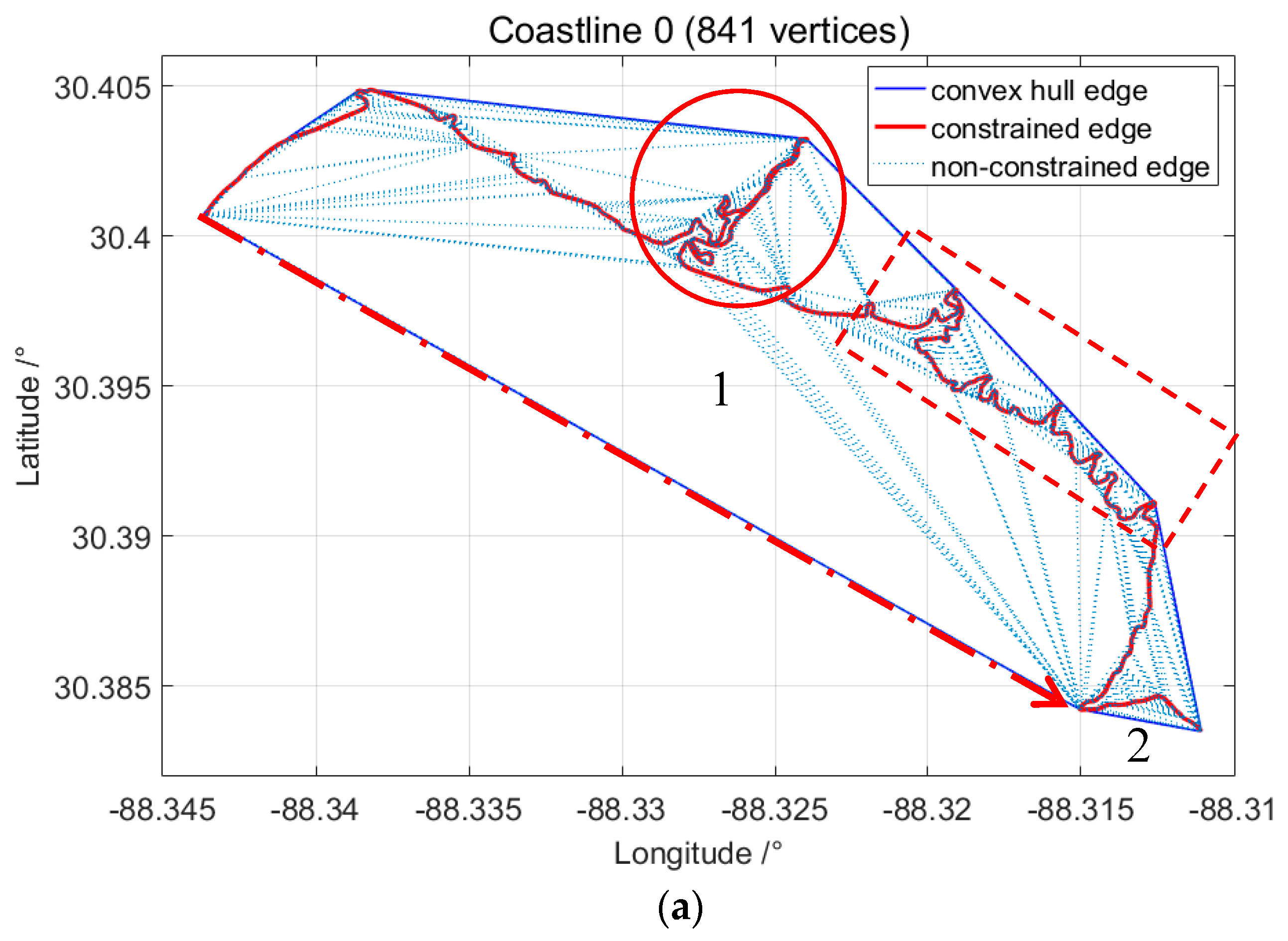
As is shown in Figure 4, three different expressions of the same coastline whose shape is relatively simple are extracted from three different ENC sheets to be used in this section.
By matching Coastline 1 and Coastline 2 with Coastline 0, they both can be seen as the generalization results from Coastline 0. When setting the direction from left to right as positive, as is shown in Figure 4 by the red dot dash arrow, there are two root-bends on the right side of each coastline, in which the bigger one, named as root-bend 1 with its baseline marked with a directed red dot dash line, has an order of magnitude advantage in area, thus playing a decisive role in shape recognition. In root-bend 1, there are two main shape details: (1) the shape bend marked by the red circle, and (2) the small bend series marked by the red dash rectangle. When comparing Coastline 0 with Coastline 1 and Coastline 2, it is easy to find that the shape details are gradually removed with the enhancement of generalization degree, while the global shape feature, or in other words, the root-bend 1’s global directionality, is scarcely changed.
2. Relatively complex coastlines
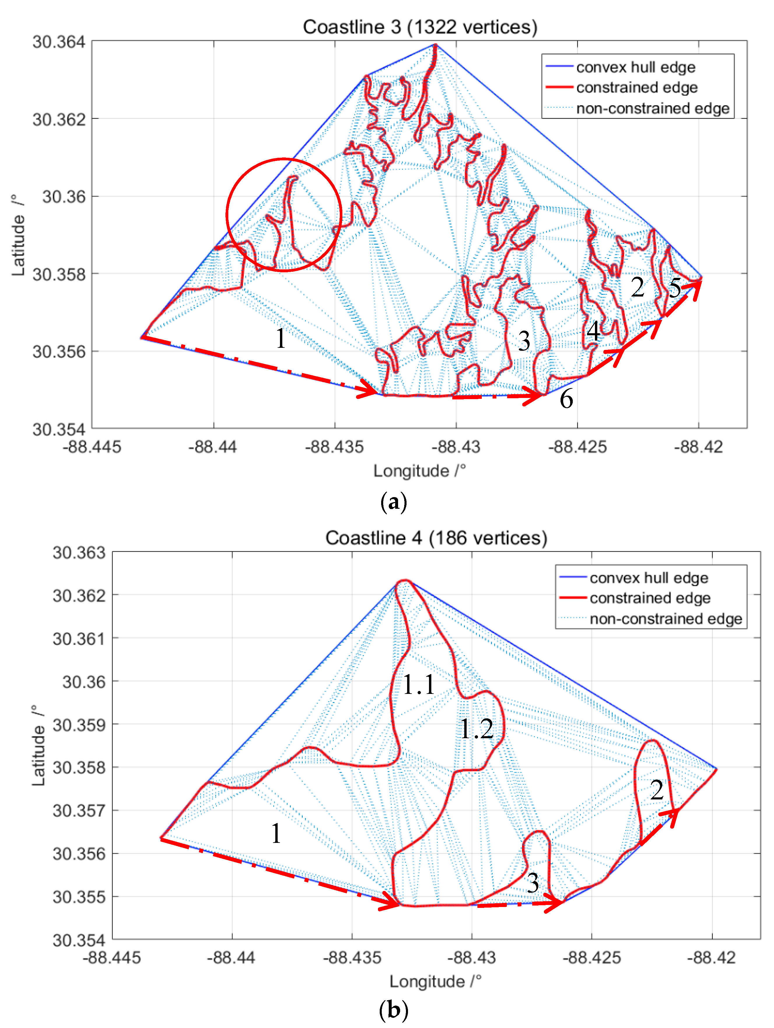
As is shown in Figure 5, two different expressions of the same coastline are extracted from two different scale ENC sheets to be used in this section. Visually, the small bends in Coastline 3 are much more than those in Coastline 0. Furthermore, the complexities shown in Table 5 show a similar result (about 1031 vs. 275), thus its shape is significantly more complex than that of Coastline 0.
Though significantly generalized, the main shape features of Coastline 3 are well retained. More specifically, when setting the positive direction as the red dotted-dashed arrows in Figure 5, the general spatial location and area proportion of the largest three root-bends on the right side of Coastline 3 are well preserved.
4.1.2. Results and Discussion
Experimental results on the two groups of coastlines above are shown in Table 5.
Taking into account the application scenarios of these methods, namely the shape similarity aspect in coastline generalization’s quality assessment, the experimental results are mainly discussed from the following two aspects:
1. The relationship between generalization degree and shape similarity degree
Theoretically, for the same coastline, correctly assessed shape similarity degree should be inversely proportional to generalization degree.
For the results shown in Table 5, and should be compared. As the scale difference between Coastline 2 and Coastline 0 is larger than that between Coastline 1 and Coastline 0, should be higher than . In this aspect, experimental results of all assessment methods are consistent with the theoretical expectation.
2. The stability of experimental results among different coastlines
As the shape similarity assessment methods are to be used in the shape similarity aspect in coastline generalization’s quality assessment, the stability among different coastlines (under the same generalization degree, or the same scale span) is one of the basic requirements. More specifically, shape similarity degrees of different coastlines under the same scale span should be close to each other, fluctuating with the complexity of their shape characteristics.
For the results shown in Table 5, as and , the shape similarity assessment results should be less than . At the same time, while , as shape complexity of Coastline 3 (1031) is much higher than that of Coastline 0 (274), should be higher than , namely the sorting result of shape similarity degrees should be:
However, except the DBF-SS presented, none of the other three methods meet this expectation. By analyzing the characteristics, including spatial span, vertices’ locations, and shape feature losses, in these coastlines, we can find the corresponding reasons:
• Hausdorff Distance
The small sharp bend in Coastline 0 marked with a red circle caused the maximum distance with Coastline 1, which is even larger than the maximum distance caused by the sharp bend marked with a red circle in Coastline 3, thus significantly affecting the result of the HD method. This phenomenon proved again that, although the usage of distance-metrics based methods like the HD in linear feature generalization’s quality assessment does have a certain significance, their usage in shape similarity assessment is not suitable.
• Length Ratio
There are much smaller sharp bends in Coastline 3 that are significantly flattened during the generalization process to generate Coastline 4, thus causing a huge drop in total length, leading to the result of the LR being significantly lower than other compared groups. This proves the limitations of the LR in measuring shape similarity among coastlines with different shape complexity.
• Turning Function
Theoretically, Turning Function is actually the definite integral of the accumulated angle difference in the length direction of the coastlines, and thus is highly related to the total length and turning angle values along the coastline. This will lead to its results being rather unstable among different coastlines. Similarly, Turning Function cannot ensure the stability of its result among different coastlines.
4.2. Experiments on Differently Generalized Coastlines
The main purpose of this part is to test the sensitivity of the experimental methods on different generalization solutions. Thus, five different coastlines, which are generalized from Coastline 4 manually, are used in this part.
4.2.1. Experimental Coastlines
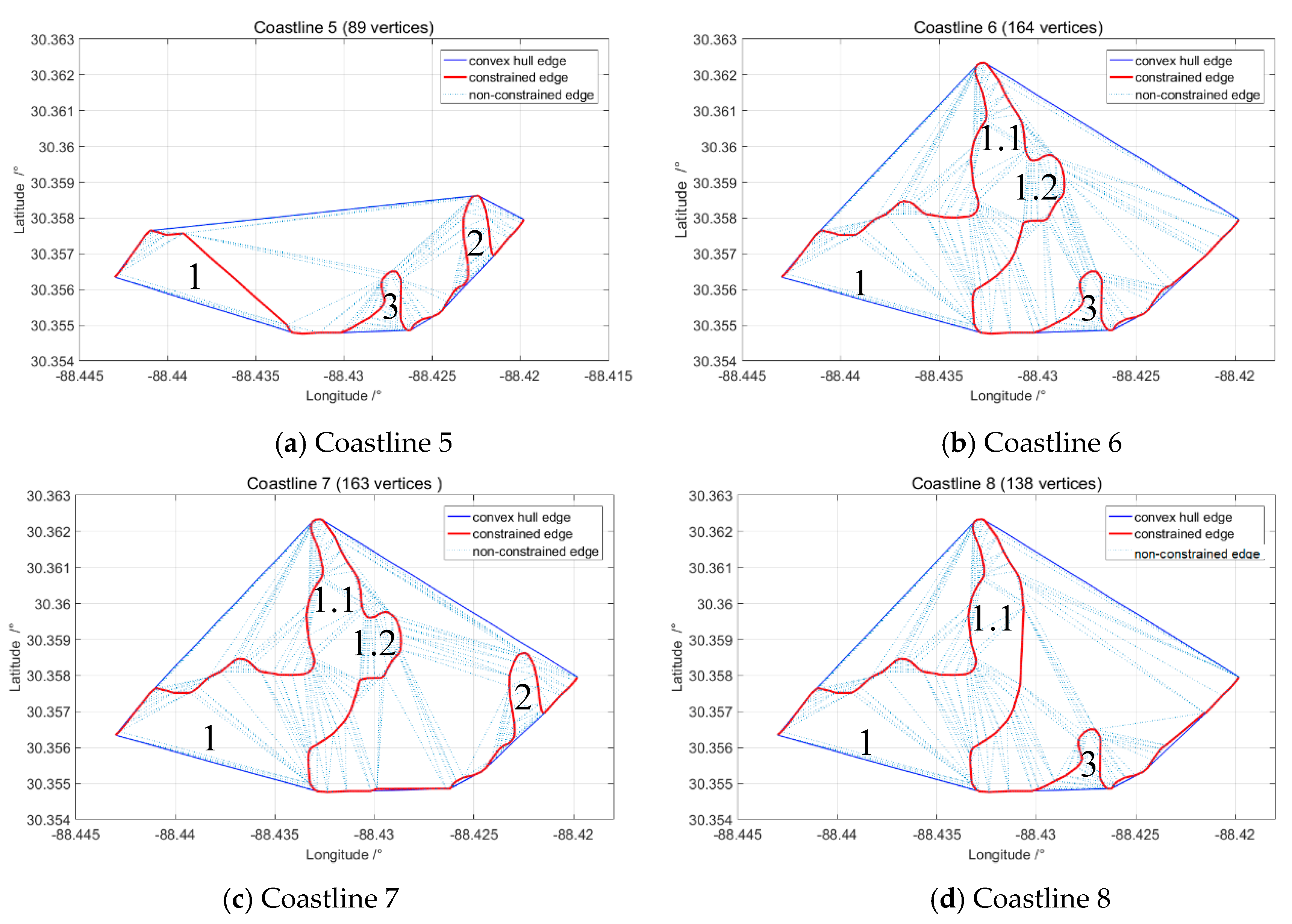
The sensitivity to possible generalization errors in coastline generalization is of great importance to coastline generalization’s shape similarity assessment methods. To test this property, four different generalization schemes on Coastline 4 are done manually to generate four different coastlines, as is shown in Figure 6.
To represent as much possible situations as possible, each root-bend in Coastline 4, including root-bend 1, root-bend 2, and root-bend 3 (sorted by their area) are generalized one by one to form three different plans: Coastlines 5, 6 and 7 to test the methods on different generalization plans. To make the generalization plans contain different scales of generalization operations, based on Coastline 6, bend 1.2, a small bend in root-bend 1 is generalized to form Coastline 8. It is worth mentioning that the results are schematic, although the quality of the automatic generalization method is still unable to be guaranteed, quality problems like the top-left one in Figure 6 usually will not happen during manual generalization.
4.2.2. Results and Discussion
To compare the experimental results with human shape recognition on Coastline 5 to 8 against Coastline 4, 10 postgraduate students majoring in map generalization including 3 PhD students and 7 master students, all with more than 2 years of experience in map generalization, are involved to sort the shape similarity of them. In order to exclude the influence of other factors, all the coastlines are print in one white paper without any coordinates with the same color and thickness. The results are shown in Table 6.
Experimental results of the assessment methods on these coastlines and their ranks (shown in parentheses) among coastlines are shown in Table 7.
Seen from the results of rank, the results of HD and TF are not consistent with people’s visual-based rank results, showing these methods’ lesser sensitivity to possible generalization errors. This phenomenon can be explained from the perspective of the experimental coastlines’ shape.
There are three main root-bends on the right side, namely root-bends 1,2 and 3, ranked with their area. Compared with Coastline 6, despite bend 1.2, one child bend of root-bend 1 is flattened in Coastline 8, and the change in Hausdorff distance caused by this part is still less than that caused by the flattening of root-bend 2. Therefore, the results of these groups are the same.
On the other side, as the generalization schemes used in this section are simply done by removing certain vertices, the accumulated angle will be significantly affected in some sections along the coastline. As a result, the rank result of the Turning Function method seems rather strange. This finding confirms another limitation of the TF method in assessing the shape similarity of coastline generalization.
As the shape similarity assessment of the presented DBF-SS is not only related to the individual bends, but also related to the hierarchical relationship among bends in the coastline, it has achieved suitable results in all experiments, which proves the usability and stability of it in coastline generalization’s shape similarity assessment among other experimental methods.
4.3. Experiment on Global Coastline Datasets
The main purpose of this part is to further testify to the applicability of all experimental methods among different scales and coastlines. To ensure that every coastline in each dataset has corresponding records in the other two datasets, only the 10 longest coastlines are extracted from each dataset to be the experimental data in this subsection.
4.3.1. Experimental Coastlines
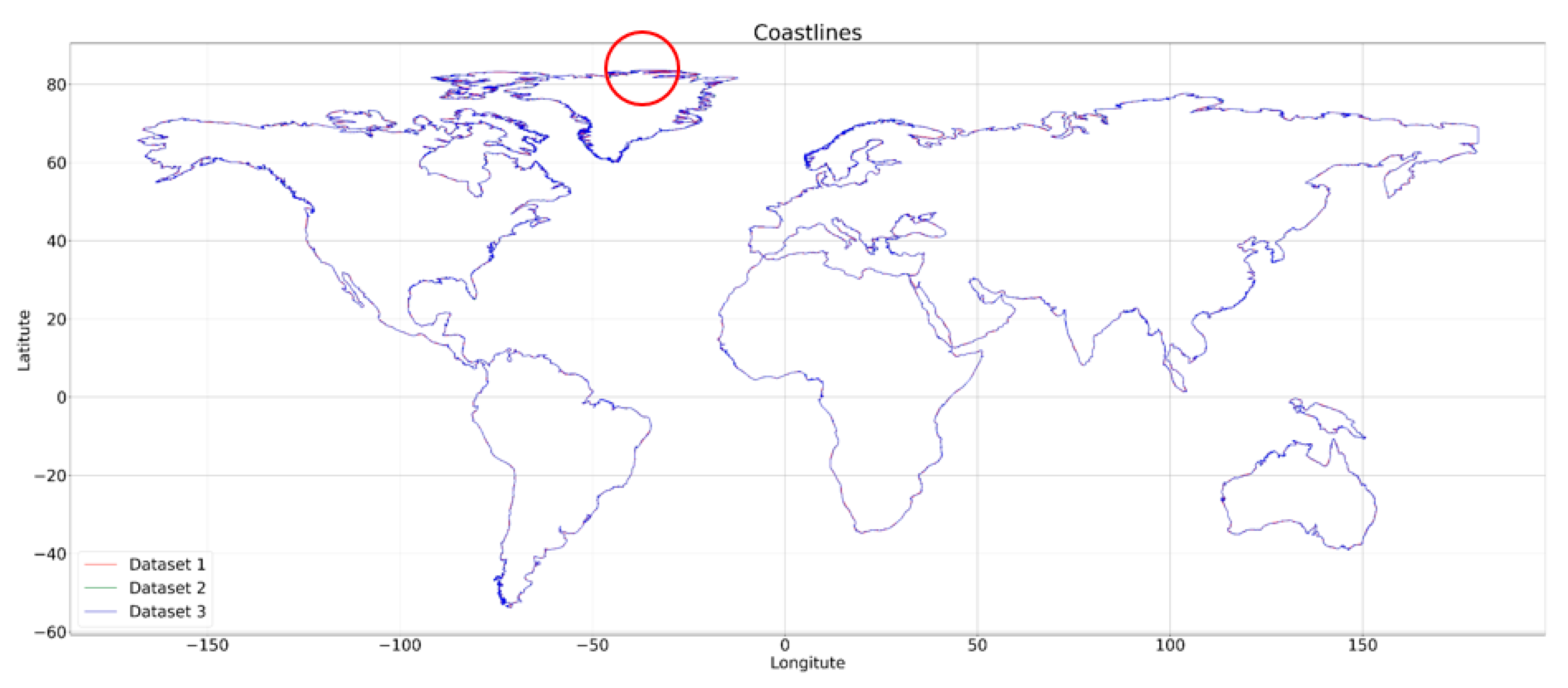
As is shown in Figure 7, all experimental coastlines are the closed boundaries of the main continents and very big islands (e.g., Greenland). Perhaps due to the differences in importance degree, shape features of these coastlines are rather rich, ranging from relatively flat coastlines (e.g., coastline in southwestern Africa) to extremely tortuous ones (e.g., coastline of Greenland). Therefore, this part of experiment can be used to validate the applicability of experimental methods among coastlines of different shape features. Generally, although shape details are compressed heavily in Figure 7 due to the limitation of the paper size, we still can find shape differences among experimental datasets ununiformed: the coastlines of southwestern Africa are highly coincident, while the ones of Greenland are quite different in shape.
By looking into the details of Table 4a, the following conclusions can be drawn:
- (1)
- The longest 10 coastline features encircled more than 90% of the land area on Earth in each dataset.
- (2)
- With the reduction of scale, the complexity of the coastline is also greatly reduced.
4.3.2. Results and Discussion
Experimental results of the assessment methods on the two groups of coastlines above are shown in Table 8, in which all the average indexes are calculated by:
where is the shape similarity index between coastline , and other parameters are the same as above.
Generally, from the level of the whole dataset, the experimental results should decrease with the vertex reserve also decreasing, as is explained in Section 4.1.2. From this point of view, all of the results are decreasing with the generalization degree increasing. However, by comparing the results of each method in different datasets, we can find that the difference between the results of the Average HD is rather small (about 0.01°), while, for other methods, the results show their strong applicability on large datasets. By looking back at every coastline in these datasets, we can find that there exists a complex segment in Greenland’s coastline, whose spatial location change has an order of magnitude than others (marked by the red circle in Figure 7), and thus causes the results of Average HD to be rather close to each other, which again proves that the usage of distance-metric based methods in shape similarity assessment is not suitable.
5. Conclusions
Shape similarity assessment is of great importance in quality assessment of coastline generalization. However, research in this field is still insufficient.
In this paper, a hierarchical coastline’s shape representation model, the Dual-side Bend Forest, is presented. Firstly, coastlines are divided into a pair of bend sequences by using the CDT and Convex Hull theory. After bend division, the shape features are treated specifically by allocating the bends’ weights in the DBF according to the area distribution of them in a layer by layer pattern. Then, the shape similarity among coastlines of different scales is calculated in a hierarchical pattern. By introducing the relative spatial locational relationship among bends of the same layer, the overall shape features are assembled into one single function. In this way, the shape similarity between two coastlines is computed as the sum of all the differences between corresponding bends. Experiments on different groups of coastlines indicate the advantages of the DBF-SS in usability on this shape similarity assessment, stability among coastlines and sensitivity in generalization errors.
Nonetheless, there is still room for improvement in this method: the partial shape similarity assessment problem. In this paper, the integrity of all generalized coastlines is guaranteed. However, the destruction of data integrity may occur in some cases, for example, some coastlines may be cut from the middle part to maintain the right topological relation, while some others may be cut at the edge of the new map. Therefore, how to deal with such problems is one of the major issues in our future research.
Author Contributions
Z.L., J.Z., and F.W. conceived and designed the study. Z.L. performed the experiments and wrote the paper. All authors read and approved the manuscript.
Funding
This research was funded by the National Key Research and Development Program of China Grant No. 2016YFC1401203.
Acknowledgments
I want to take this opportunity to thank my schoolmates Bo Zou, Le Yang, Guangchao Hou, Junpeng Zhao, Kangzhuang Liang, Zhehan Mou, Chong Zhang, Huiqiang Lu, Feifei Song and Zhe Zhang, who helped to run the human shape recognition experiment in this paper responsibly.
Conflicts of Interest
The authors declare no conflict of interest.
References
- Raposo, P. Scale-specific automated line simplification by vertex clustering on a hexagonal tessellation. Cartogr. Geogr. Inf. Sci. 2013, 40, 427–443. [Google Scholar] [CrossRef]
- Li, Z. Algorithmic Foundation of Multi-Scale Spatial Representation; CRC Press: Boca Raton, FL, USA, 2008. [Google Scholar]
- Silavisesrith, W.; Silavisesrith, W. Multicriteria Generalization MCG: A Decision-Making Framework for Formalizing Multiscale Environmental Data Reduction; Taylor & Francis, Inc.: Oxfordshire, UK, 2012. [Google Scholar]
- Dougla, D.H.; Peucker, T.K. Algorithms for the Reduction of the Number of Points Required to Represent a Digital Line or Its Caricature. Can. Cartogr. 1973, 10, 112–122. [Google Scholar] [CrossRef]
- Li, Z.; Openshaw, S. Algorithms for automated line generalization 1 based on a natural principle of objective generalization. Int. J. Geogr. Inf. Syst. 1992, 6, 373–389. [Google Scholar] [CrossRef]
- Bresson, X.; Esedoḡlu, S.; Vandergheynst, P.; Thiran, J.P.; Osher, S. Fast Global Minimization of the Active Contour/Snake Model. J. Math. Imaging Vis. 2007, 28, 151–167. [Google Scholar] [CrossRef] [Green Version]
- Guilbert, E.; Saux, E. Cartographic generalisation of lines based on a B-spline snake model. Int. J. Geogr. Inf. Sci. 2008, 22, 847–870. [Google Scholar] [CrossRef]
- Plazanet, C. Modelling Geometry for Linear Feature Generalization; Bridging the Atlantic, Taylor & Francis: Oxfordshire, UK, 1997; pp. 264–279. [Google Scholar]
- Wang, Z.; Müller, J.C. Line Generalization Based on Analysis of Shape Characteristics. Cartogr. Geogr. Inf. Syst. 1998, 25, 3–15. [Google Scholar] [CrossRef]
- Ai, T.; Zhou, Q.; Zhang, X.; Huang, Y.; Zhou, M. A Simplification of Ria Coastline with Geomorphologic Characteristics Preserved. Mar. Geod. 2014, 37, 167–186. [Google Scholar] [CrossRef]
- Plazanet, C.; Affholder, J.G.; Fritsch, E. The Importance of Geometric Modeling in Linear Feature Generalization. Am. Cartogr. 2013, 22, 291–305. [Google Scholar] [CrossRef]
- Ehrliholzer, R. Quality assessment in generalization: Integrating quantitative and qualitative methods. In Proceedings of the 17th International Cartographic Conference, Barcelona, Spain, 3–9 September 1995. [Google Scholar]
- Yan, H.; Li, J. Spatial Similarity Relations in Multi-Scale Map Spaces; Springer International Publishing: Cham, Switzerland, 2014. [Google Scholar]
- Su, B.; Li, Z.; Lodwick, G. Morphological Models for the Collapse of Area Features in Digital Map Generalization. Geoinformatica 1998, 2, 359–383. [Google Scholar] [CrossRef]
- Chehreghan, A.; Abbaspour, R.A. An assessment of spatial similarity degree between polylines on multi-scale, multi-source maps. Geocarto Int. 2016, 32, 471–487. [Google Scholar] [CrossRef]
- Plazanet, C. Measurement, characterization and classification for automated line feature generalization. In Proceedings of the Twelfth International Symposium on Computer-Assisted Cartography, Charlotte, NC, USA, 27–29 February 1995. [Google Scholar]
- Hong, B.; Soatto, S. Shape Matching using Multiscale Integral Invariants. IEEE Trans. Pattern Anal. Mach. Intell. 2015, 37, 151. [Google Scholar] [CrossRef] [PubMed]
- Mohammadi, N.; Malek, M. VGI and Reference Data Correspondence Based on Location-Orientation Rotary Descriptor and Segment Matching. Transa. GIS 2015, 19, 619–639. [Google Scholar] [CrossRef]
- Chrobak, T.; Szombara, S.; Kozoå, K.; Lupa, M. A method for assessing generalized data accuracy with linear object resolution verification. Geocarto Int. 2016, 32, 238–256. [Google Scholar] [CrossRef]
- Huttenlocher, D.P.; Klanderman, G.A.; Rucklidge, W.A. Comparing Images Using the Hausdorff Distance. IEEE Trans. Pattern Anal. Mach. Intell. 1993, 15, 850–863. [Google Scholar] [CrossRef]
- Hangouet, J.F. Computation of the Hausdorff distance between plane vector polylines. In Proceedings of the Twelfth International Symposium on Computer-Assisted Cartography, Charlotte, NC, USA, 27–29 February 1995. [Google Scholar]
- Tsapanos, N.; Tefas, A.; Nikolaidis, N.; Pitas, I. Shape matching using a binary search tree structure of weak classifiers. Pattern Recognit. 2012, 45, 2363–2376. [Google Scholar] [CrossRef]
- Alt, H.; Godau, M. Computing the Fréchet distance between two polygonal curves. Int. J. Comput. Geom. Appl. 1995, 5, 75–91. [Google Scholar] [CrossRef]
- Ariza-López, F.J.; Mozas-Calvache, A.T. Comparison of four line-based positional assessment methods by means of synthetic data. Geoinformatica 2012, 16, 221–243. [Google Scholar] [CrossRef]
- Alt, H.; Efrat, A.; Rote, G.; Wenk, C. Matching planar maps. J. Algorithms 2003, 49, 262–283. [Google Scholar] [CrossRef]
- Iv, A.F.C.; Wenk, C. Geodesic Fréchet distance inside a simple polygon. ACM Trans. Algorithms 2008, 7, 193–204. [Google Scholar] [CrossRef]
- Buchin, M. Constrained free space diagrams: A tool for trajectory analysis. Int. J. Geogr. Inf. Sci. 2010, 24, 1101–1125. [Google Scholar] [CrossRef]
- Liu, H.; Fan, Z.; Zhen, X.; Deng, M. An Improved Local Length Ratio Method for Curve Simplification and Its Evaluation. Geogr. GeoInf. Sci. 2011, 27, 45–48. [Google Scholar]
- Zhao, Y.; Chen, Y.Q. Included angle chain: A method for curve representation. J. Softw. 2004, 15, 300–307. [Google Scholar]
- Zhang, M.; Shi, W.; Meng, L. A generic matching algorithm for line networks of different resolutions. In Proceedings of the ICA Workshop on Generalisation & Multiple Representation, A. Coruña, Spain, 7–8 July 2005; pp. 7–8. [Google Scholar]
- Arkin, E.M.; Chew, L.P.; Huttenlocher, D.P.; Kedem, K.; Mitchell, J.S. An Efficiently Computable Metric for Comparing Polygonal Shapes. IEEE Trans. Pattern Anal. Mach. Intell. 1990, 13, 209–216. [Google Scholar] [CrossRef]
- Veltkamp, R.C. Shape matching: Similarity measures and algorithms. In Proceedings of the International Conference on Shape Modeling and Applications, Genova, Italy, 7–11 May 2001; p. 188. [Google Scholar]
- Wolter, D. Spatial Representations for Mapping. In Spatial Representation and Reasoning for Robot Mapping; Springer: Berlin/Heidelberg, Germany, 2008; pp. 19–52. [Google Scholar]
- Abbaspour, R.A.; Chehreghan, A.; Karimi, A. Assessing the efficiency of shape-based functions and descriptors in multi-scale matching of linear objects. Geocarto Int. 2018, 33, 879–892. [Google Scholar] [CrossRef]
- Persoon, E.; Fu, K.S. Shape Discrimination Using Fourier Descriptors. IEEE Trans. Syst. Man Cybern. 1986, 7, 170–179. [Google Scholar] [CrossRef]
- Fritsch, E.; Lagrange, J.P. Spectral representations of linear features for generalization. In Proceedings of the International Conference on Spatial Information Theory; Springer: Berlin/Heidelberg, Germany, 1995; pp. 157–171. [Google Scholar]
- Gasquet, C.; Witomski, P. Analyse de Fourier et Applications: Filtrage, Calcul Numérique, Ondelettes; Dunod: Paris, France, 1990; pp. 187–209. [Google Scholar]
- Chuang, G.H.; Kuo, C.J. Wavelet description of planar curves. IEEE Trans. Image Process. 1996, 5, 56–70. [Google Scholar] [CrossRef] [PubMed]
- Chansophea, C.; Sumanta, G.; Paul, J. Simplipoly: Curvature-based polygonal curve simplification. Int. J. Comput. Geom. Appl. 2011, 21, 417–429. [Google Scholar]
- Alexanderson, G.L. Mathematical People: Profiles and Interviews; CRC Press: Boca Raton, FL, USA, 2008; ISBN 978-1-56881-340-0. [Google Scholar]
- Goodchild, M.F. Fractals and the accuracy of geographical measures. Math. Geosci. 1980, 12, 85–98. [Google Scholar] [CrossRef]
- Goodchild, M.F.; Mark, D.M. The Fractal Nature of Geographic Phenomena. Ann. Assoc. Am. Cartogr. 1987, 77, 265–278. [Google Scholar] [CrossRef]
- Jiang, J.; Plotnick, R.E. Fractal Analysis of the Complexity of United States Coastlines. Math. Geosci. 1998, 30, 535–546. [Google Scholar]
- Dutton, G.H. Fractal Enhancement of Cartographic Line Detail. Am. Cartogr. 1981, 8, 23–40. [Google Scholar] [CrossRef]
- Ren, Y.; Tang, J.; Wu, S. Geometric properties preserved line simplification algorithm based on fractal. In Proceedings of the IEEE International Geoscience and Remote Sensing Symposium, Vancouver, BC, Canada, 24–29 July 2011; pp. 3019–3022. [Google Scholar]
- Kullback, S. The Kullback-Leibler Distance. Am. Stat. 1987, 41, 340–341. [Google Scholar]
- Marascuilo, L.A.; Slaughter, R.E. Statistical Procedures for Identifying Possible Sources of Item Bias based on x2 Statistics. J. Educ. Meas. 1981, 18, 229–248. [Google Scholar] [CrossRef]
- Belongie, S.J.; Malik, J.; Puzicha, J. Shape Matching and Object Recognition Using Shape Contexts. In Proceedings of the IEEE International Conference on Computer Science and Information Technology, Chengdu, China, 9–10 July 2010; pp. 483–507. [Google Scholar]
- Mortensen, E.N.; Deng, H.; Shapiro, L. A SIFT Descriptor with Global Context. In Proceedings of the 2005 IEEE Computer Society Conference on Computer Vision and Pattern Recognition (CVPR’05), San Diego, CA, USA, 20–25 June 2005; pp. 184–190. [Google Scholar]
- Belongie, S.; Malik, J.; Puzicha, J. Matching shapes. In Proceedings of the Eighth IEEE International Conference on Computer Vision (ICCV 2001), Vancouver, BC, Canada, 7–14 July 2001; pp. 454–461. [Google Scholar]
- Attneave, F. Some informational aspects of visual perception. Psychol. Rev. 1954, 61, 183. [Google Scholar] [CrossRef] [PubMed]
- Hoffman, D.D.; Richards, W.A. Representing Smooth Plane Curves for Recognition: Implications for Figure-Ground Reversal. In Proceedings of the National Conference on Artificial Intelligence, Pittsburgh, PA, USA, 18–20 August 1982; pp. 5–8. [Google Scholar]
- Thapa, K. Data compression and critical points detection using normalized symmetric scattered matrix. Autocarto 1989, 9, 78–89. [Google Scholar]
- Ai, T.; Guo, R.; Liu, Y. A Binary Tree Representation of Curve Hierarchical Structure in Depth. Acta Geod. Cartogr. Sin. 2001, 30, 343–348. [Google Scholar]
- Chrobak, T.; Lupa, M.; Szombara, S.; Dejniak, D. The use of cartographic control points in the harmonization and revision of MRDBs. Geocarto Int. 2017, 32, 1–27. [Google Scholar] [CrossRef]
- Zhu, P.; Chirlian, P.M. On Critical Point Detection of Digital Shapes. IEEE Trans. Pattern Anal. Mach. Intell. 1995, 17, 737–748. [Google Scholar]
- Nakos, B.; Miropoulos, V. Local length ratio as a measure of critical points detection for line simplification. In Proceedings of the Fifth Workshop on Progress in Automated Map Generalization, Paris, France, 28–30 April 2003. [Google Scholar]
- Qian, H.; Zhang, M.; Wu, F. A New Simplification Approach Based on the Oblique-Dividing-Curve Method for Contour Lines. ISPRS Int. J. GeoInf. 2016, 5, 153. [Google Scholar] [CrossRef]
- Aurenhammer, F.; Klein, R.; Lee, D.-T. Voronoi Diagrams and Delaunay Triangulations; World Scientific Publishing Company: Singapore, 2013. [Google Scholar]
- Buttenfield, B.P.; McMaster, R.B. Map Generalization: Making Rules for Knowledge Representation, 1st ed.; Longman Scientific & Technical: London, UK, 1991. [Google Scholar]
- Seki, M.; Shimizu, T.; Matsumoto, K. Part-Based Representations of Visual Shape and Implications for Visual Cognition. Adv. Psychol. 2001, 130, 401–459. [Google Scholar] [Green Version]
- Ai, T.; Shuai, Y.; Li, J. The Shape Cognition and Query Supported by Fourier Transform. In Proceedings of the Headway in Spatial Data Handlng International Symposium on Spatial Data Handling, Montpellier, France, 23–25 July 2008; pp. 39–54. [Google Scholar]
- Zhai, J.; Li, Z.; Wu, F.; Xie, H.; Zou, B. Quality Assessment Method for Linear Feature Simplification Based on Multi-Scale Spatial Uncertainty. Int. J. GeoInf. 2017, 6, 184. [Google Scholar] [CrossRef]
- Perkal, J.D. An Attempt at Objective Generalization; Michigan Inter-University: Ann Arbor, MI, USA, 1965; pp. 130–142. [Google Scholar]
- Christensen, A.H.J. Line Generalization by Waterlining and Medial-Axis Transformation. Successes and Issues in an Implementation of Perkal’s Proposal. Cartogr. J. 2000, 37, 19–28. [Google Scholar] [CrossRef]
- Cao, Z.; Li, M.; Cheng, L. Multi-way trees representation for curve bends. Acta Geod. Cartogr. Sin. 2013, 42, 602–607. [Google Scholar]
- Kobayakawa, M.; Kinjo, S.; Hoshi, M.; Ohmori, T.; Yamamoto, A. Fast Computation of Similarity Based on Jaccard Coefficient for Composition-Based Image Retrieval. In Proceedings of the Advances in Multimedia Information Processing—PCM 2009, Pacific Rim Conference on Multimedia, Bangkok, Thailand, 15–18 December 2009; pp. 949–955. [Google Scholar]
Figure 1.
Shape parameters of bend.
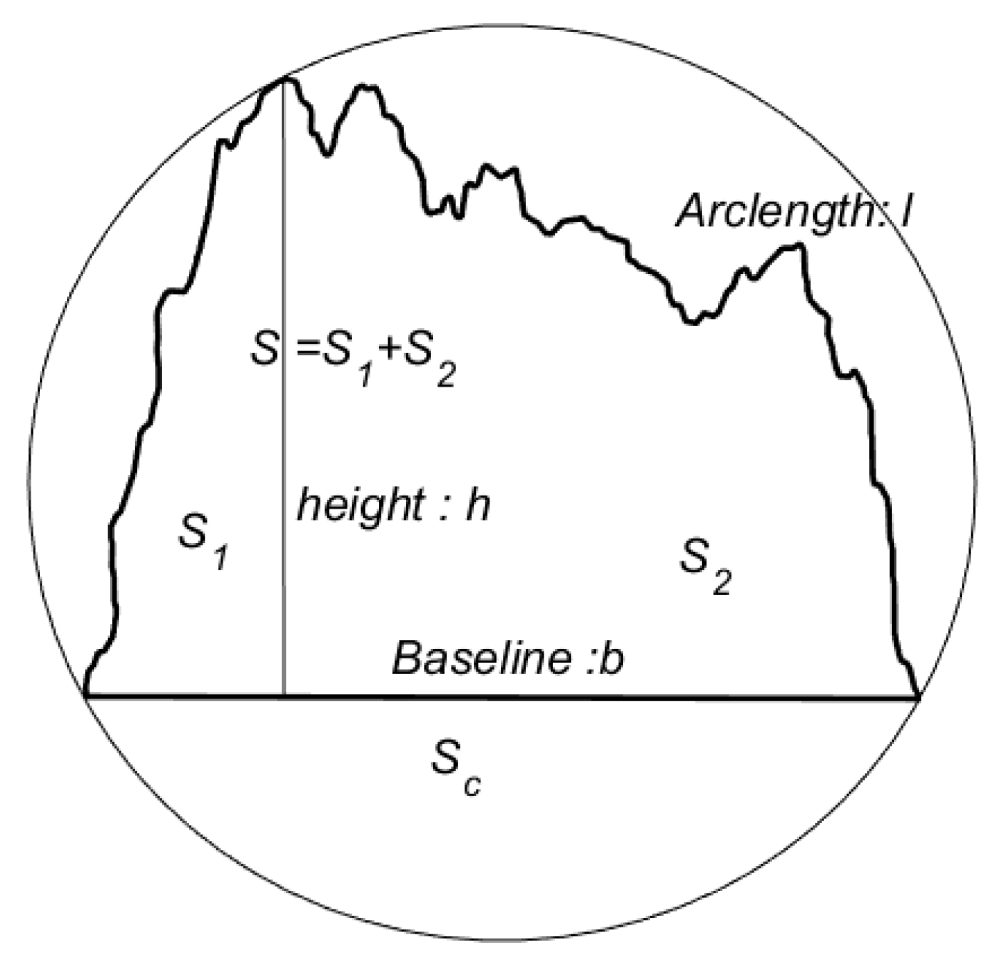
Figure 2.
Sample coastline and its CDT.
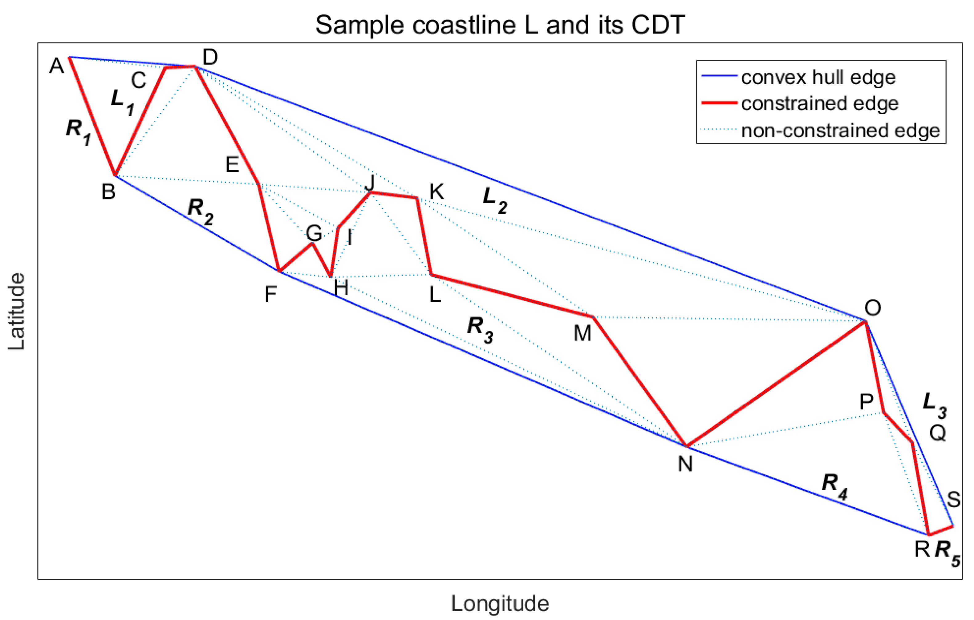
Figure 3.
DBF of sample coastline . (a) ’s left-side bend forest; (b) ’s right-side bend forest.

Figure 4.
Relatively simple coastline segments. (a) Coastline 0; (b) Coastline 1; (c) Coastline 2.

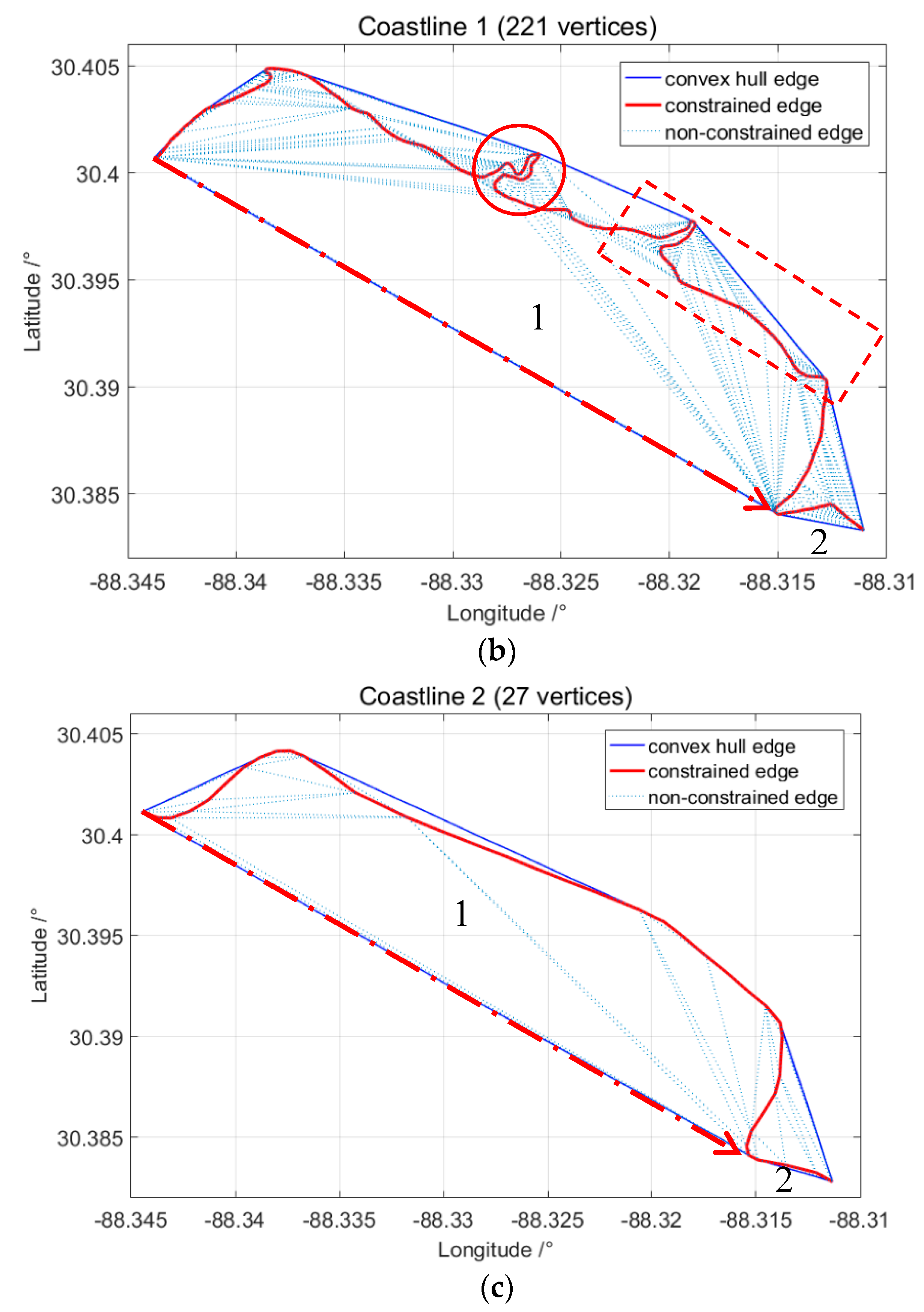
Figure 5.
Relatively complex coastline segments. (a) Coastline 3; (b) Coastline 4.

Figure 6.
Manually generalized coastlines.

Figure 7.
Coastline datasets.

Table 1.
Famous complex geometry parameter-based methods.
| Method | Shape Similarity Parameter | Drawbacks |
|---|---|---|
| IAC | Euclidean distance among sequences of equal-length line segments | Equally division of linear features |
| ADI | Integration difference of azimuthal angle of the linear feature | Usability on smooth linear features |
| TF | Integration of cumulative angle function along the linear feature | The homologous points’ exact matching |
Table 2.
Delaunay triangulation division.
| Type | Classification Basis | Role |
|---|---|---|
| I | Peripheral triangle | |
| II | and | Bend bottom |
| III | and | Bend’s decomposed part |
| IV | and | Bend’s branch part |
Table 3.
Shape parameters of bend.
| Shape Parameters | Meaning |
|---|---|
| Baseline length | |
| Height | |
| Arc length | |
| Curvature degree | |
| Symmetry |
Table 4.
Basic information of experimental datasets.
(a) Extracted coastlines.
| Coastline | Scale | Vertex Number | Total Length/10−4° | Complexity |
|---|---|---|---|---|
| Coastline 0 | 1:40,000 | 841 | 837.97 | 274.97 |
| Coastline 1 | 1:80,000 | 221 | 598.11 | 218.36 |
| Coastline 2 | 1:350,000 | 27 | 469.45 | 203.23 |
| Coastline 3 | 1:40,000 | 1322 | 1259.31 | 1031.35 |
| Coastline 4 | 1:80,000 | 186 | 483.07 | 480.65 |
(b) Manually generalized coastlines.
| Coastline | Vertex Number | Total Length/10−4° | Complexity |
|---|---|---|---|
| Coastline 5 | 89 | 305.73 | 521.21 |
| Coastline 6 | 164 | 450.81 | 448.55 |
| Coastline 7 | 163 | 459.63 | 457.33 |
| Coastline 8 | 138 | 419.28 | 417.18 |
(c) Global coastline datasets.
| Dataset | Type | Feature Number | Vertex Number | Length/° | Complexity |
|---|---|---|---|---|---|
| Dataset 1 | Total | 179,837 | 9,453,089 | 20,686.97 | 0.94 |
| Selected | 10 | 3,378,200 | 8032.60 | 0.38 | |
| Dataset 2 | Total | 32,830 | 340,359 | 14,953.70 | 0.68 |
| Selected | 10 | 100,416 | 6669.76 | 0.32 | |
| Dataset 3 | Total | 742 | 7282 | 6225.56 | 0.28 |
| Selected | 10 | 3026 | 3809.68 | 0.18 |
Table 5.
Experiment results on Coastlines 0–4.
| Compare/Compared Coastline | Vertex Reserved (%) | HD (10−4°) | LR (%) | TF | DBF-SS (%) | |
|---|---|---|---|---|---|---|
| Coastline 0 | Coastline 1 | 26.28 | 30.94 | 71.38 | 84.30 | 78.87 |
| Coastline 2 | 3.21 | 51.56 | 56.02 | 94.53 | 41.37 | |
| Coastline 3 | Coastline 4 | 14.07 | 23.37 | 38.36 | 118.83 | 53.59 |
Table 6.
Generalization schemes of Coastlines 5–8.
| Coastlines | Generalization Schemes | Shape Similarity Rank |
|---|---|---|
| Coastline 5 | Root-bend 1 is almost totally flattened | 4th |
| Coastline 6 | Root-bend 2 is flattened | 2nd |
| Coastline 7 | Root-bend 3 is flattened | 1st |
| Coastline 8 | Root-bend 2 and bend 1.1 is flattened | 3rd |
Table 7.
Experimental results and ranks.
| Compare/Compared Coastlines | HD (10−4°) | LR (%) | TF | DBF-SS (%) | |
|---|---|---|---|---|---|
| Coastline 4 | Coastline 5 | 69.56 (4) | 63.29 (4) | 86.08 (3) | 34.38 (4) |
| Coastline 6 | 20.35 (2) | 93.32 (2) | 86.82 (4) | 86.22 (2) | |
| Coastline 7 | 16.49 (1) | 95.15 (1) | 65.99 (1) | 91.16 (1) | |
| Coastline 8 | 20.35 (2) | 86.79 (3) | 75.92 (2) | 83.38 (3) | |
Table 8.
Experiment results on three datasets.
| Compare/Compared Coastline | Vertex Reserved (%) | Average HD (°) | Average LR (%) | Average TF | Average DBF-SS (%) | |
|---|---|---|---|---|---|---|
| Dataset 1 | Dataset 2 | 2.97 | 1.28 | 83.03 | 12.64 | 89.73 |
| Dataset 3 | 0.09 | 1.29 | 47.43 | 37.79 | 72.35 | |
© 2018 by the authors. Licensee MDPI, Basel, Switzerland. This article is an open access article distributed under the terms and conditions of the Creative Commons Attribution (CC BY) license (http://creativecommons.org/licenses/by/4.0/).
Share and Cite
MDPI and ACS Style
Li, Z.; Zhai, J.; Wu, F. Shape Similarity Assessment Method for Coastline Generalization. ISPRS Int. J. Geo-Inf. 2018, 7, 283. https://doi.org/10.3390/ijgi7070283
AMA Style
Li Z, Zhai J, Wu F. Shape Similarity Assessment Method for Coastline Generalization. ISPRS International Journal of Geo-Information. 2018; 7(7):283. https://doi.org/10.3390/ijgi7070283
Chicago/Turabian StyleLi, Zhaoxing, Jingsheng Zhai, and Fang Wu. 2018. "Shape Similarity Assessment Method for Coastline Generalization" ISPRS International Journal of Geo-Information 7, no. 7: 283. https://doi.org/10.3390/ijgi7070283
Note that from the first issue of 2016, this journal uses article numbers instead of page numbers. See further details here.